Conditional inference in parametric models

Abstract

This paper presents a new approach to conditional inference, based on the simulation of samples conditioned by a statistics of the data. Also an explicit expression for the approximation of the conditional likelihood of long runs of the sample given the observed statistics is provided. It is shown that when the conditioning statistics is sufficient for a given parameter, the approximating density is still invariant with respect to the parameter. A new Rao-Blackwellisation procedure is proposed and simulation shows that Lehmann Scheffé Theorem is valid for this approximation. Conditional inference for exponential families with nuisance parameter is also studied, leading to Monte carlo tests. Finally the estimation of the parameter of interest through conditional likelihood is considered. Comparison with the parametric bootstrap method is discussed.

Keywords: Conditional inference, Rao Blackwell Theorem, Lehmann Scheffé Theorem, Exponential families, Nuisance parameter, Simulation.

1 Introduction and context

This paper explores conditional inference in parametric models. A comprehensive overview on this area is the illuminating review paper by Reid (1995) [27]. Our starting point is as follows: given a model $\mathcal{P}$ defined as a collection of continuous distributions $P_{\theta}$ on $\mathbb{R}^{d}$ , with density $p_{\theta}$ where the parameter $\theta$ belongs to some subset $\Theta$ in $\mathbb{R}^{s}$ and given a sample of independent copies of a random variable with distribution $P_{\theta_{T}}$ for some unknown value $\theta_{T}$ of the parameter, we intend to provide some inference about $\theta_{T}$ conditioning on some statistics of the data. The situations which we have in mind are of two different kinds.

The first one is the Rao-Blackwellisation of estimators, which amounts to reduce the variance of an unbiased estimator by conditioning on any statistics; it is a known fact that such method reduces its variance; when the conditioning statistics is complete and sufficient for the parameter then this procedure provides optimal reduction, as stated by Lehmann-Scheffé Theorem. This realm of questions is the motivation for the first part of this paper:

1. is it possible to provide good approximations for the density of a sample conditioned on a given statistics, and, when applied for a model where some sufficient statistics for the parameter is known, does sufficiency w.r.t. the parameter still holds for the approximating density?

2. in the case when the first question has positive answer, is it possible to simulate samples according to the approximating density, and to propose some Rao-Blackwellised version for a given preliminary estimator? Also we would hope that the proposed method would be feasible, that the programming burden would be light, that the run time for this method be short, and that the involved techniques would keep in the range of globally known ones by the community of statisticians.

The second application of conditional inference pertains to the role of conditioning in models with nuisance parameters. There is a huge bibliography on this topic, some of which will be considered in details in the sequel. The usual frame for this field of problems is the exponential families one, for reasons related both with the importance of these models in applications and on the role of the concept of sufficiency when dealing with the notion of nuisance parameter. Conditioning on a sufficient statistics for the nuisance parameter produces a new exponential family, which gets free of this parameter, and allows for simple inference on the parameter of interest, at least in simple cases. This will also be discussed, since the reality, as known, is not that simple, and since so many complementary approaches have been developped over decades in this area. Using the approximation of the conditional density in this context and performing simulations yields Monte Carlo tests for the parameter of interest, free from the nuisance parameter. Also conditional maximum likelihood estimators will be produced. Comparison with the parametric bootstrap will also be discussed.

This paper is organized as follows. Section 2 describes a general approximation scheme for the conditional density of long runs of subsamples conditioned on a statistics, with explicit formulas. The (rather lengthy) proof of the main result of this section is presented in Broniatowski and Caron(2011)[4]. Discussion about implementation is provided. Section 3 presents two aspects of the approximating conditional scheme: we first show on examples that sufficiency is kept under the approximating scheme and, second, that this yields to an easy Rao-Blackwellisation procedure. An illustration of Lehmann-Scheffé Theorem is presented. Section 4 deals with models with nuisance parameters in the context of exponential families. We have found it useful to spend a few paragraphs on bibliographical issues. We address Monte Carlo tests based on the simulation scheme; in simple cases its performance is similar to that of parametric bootstrap; however conditional simulation based tests improve clearly over parametric bootstrap procedure when the test pertains to models for which the likelihood is multimodal with respect to the nuisance parameter; an example is provided. Finally we consider conditioned maximum likelihood based on the approximation of the conditional density; in simple cases its performance is similar to that of unconditional likelihood; however when the preliminary estimator of the nuisance is difficult to obtain, for example when it depends strongly on some initial point for a Newton-Raphson routine (this is indeed a very common situation), then, by the very nature of sufficiency, conditional inference based on the proxy of the conditional likelihood performs better; this is illustrated with examples.

2 The approximate conditional density of the sample

Most attempts which have been proposed for the approximation of conditional densities stem from arguments developped in Lehmann (1986)[16] for inference on the parameter of interest in models with nuisance parameter; however the proposals in this direction hinge at the approximation of the distribution of the sufficient statistics for the parameter of interest given the observed value of the sufficient statistics of the nuisance parameter. We will present some of these proposals in the section devoted to exponential families. To our knowledge, no attempt has been made to approximate the conditional distribution of a sample (or of a long subsample) given some observed statistics.

However, generating samples from the conditional distribution itself (such samples are often called co-sufficient samples, following Lockhart et al.(2007) [20]) has been considered by many authors; see for example Engen and Lillegard (1997)[12], Lindqvist et al. (2003)[17] and references therein, and Lindqvist and Taraldsen (2005)[18].

In Engen and Lillegard (1997)[12], simulating exponential or normal samples under the given value of the empirical mean is proposed. For example under the exponential distribution $Exp(\theta),$ the minimal sufficient statistics for $\theta$ is the sum of the observations, say $t_{n};$ a co-sufficient sample $x^{\ast}$ can be created by generating an $x^{{}^{\prime}}$-sample from $Exp(1)$ and taking $x_{i}^{\ast}=x_{i}^{{}^{\prime}}t_{n}/\overline{x}^{{}^{\prime}}.$ However, this approach may be at odd in simple cases, as for the Gamma density in the non exponential case.

Lockhart et al. (2007)[20] proposed a different framework based on the Gibbs sampler, simulating the conditioned sample one at a time through a sequential procedure. The example which is presented is for the Gamma distribution under the empirical mean, but it seems to perform well, for location parameter, when the true parameter is in some range, therefore not uniformly on the model. Their paper contains a comparative study with the parametric bootstrap procedure (introduced by Efron (1979)[11]) for similar problems. In a simple case, they argue favorably for both methods. We will turn back to parametric bootstrap in relation with conditional likelihood estimators, in the last section of this paper.

Other techniques have been developped in specific cases: for the inverse gaussian distribution see O’Reilly and Gravia-Medrano (2006)[22], Cheng (1984) [8]; for the Weibull distribution see Lockhart et Stephens (1994)[21]. No unified technique exists in the litterature which would work under general models.

2.1 Approximation of conditional densities

2.1.1 Notation and hypotheses

For sake of clearness we consider the case when the model $\mathcal{P}$ is a family of distributions on $\mathbb{R}$. Extension to $\mathbb{R}^{d},d>1$ can be achieved in the same way, using similar results developed in futur work.

Denote $\mathbf{X}_{1}^{n}:=\left(\mathbf{X}_{1}\mathbf{,..,X}_{n}\right)$ a set of $n$ independent copies of a real random variable $\mathbf{X}$ with density $p_{\mathbf{X},\theta_{T}}$ on $\mathbb{R}$. Let $\mathbf{x}_{1}^{n}:=\left(\mathbf{x}_{1},...,\mathbf{x}_{n}\right)$ denote the observed values of the data, each $\mathbf{x}_{i}$ resulting from the sampling of $\mathbf{X}_{i}.$ Define the r.v. $\mathbf{U}:=u\left(\mathbf{X}\right)$ and $\mathbf{U}_{1,n}:=u\left(\mathbf{X}_{1}\right)+...+u\left(\mathbf{X}_{n}\right)$ where $u$ is a real-valued measurable function on $\mathbb{R}$, and, accordingly, $u_{1,n}:=u\left(\mathbf{x}_{1}\right)+...+u\left(\mathbf{x}_{n}\right).$ Denote $p_{\mathbf{U},\theta_{T}}$ the density of the r.v. $\mathbf{U}.$ We consider approximations of the density of the vector $\mathbf{X}_{1}^{k}=\left(\mathbf{X}_{1}\mathbf{,..,X}_{k}\right)$ on $\mathbb{R}$ when $\mathbf{U}_{1,n}=u_{1,n}.$ It will be assumed that the observed value $u_{1,n}$ is ”typical”, in the sense that it keeps in the range of the iterated logarithm law order of magnitude (for large $n$). Large deviation cases could also be handled, but conditional inference is based on the implicit assumption that such cases are excluded from the analysis. We hence assume

$$\lim\sup_{n\rightarrow\infty}\frac{\left|u_{1,n}-nE[u\left(\mathbf{X}\right)]\right|}{\sqrt{Var(u\left(\mathbf{X}\right))}\sqrt{2n\log\log n}}=1.$$ (LIL)

We propose an approximation for

$$p_{u_{1,n},\theta_{T}}\left(x_{1}^{k}\right):=p_{\theta_{T}}(x_{1}^{k}|\mathbf{U}_{1,n}=u_{1,n})$$ (1)

where $\mathbf{X}_{1}^{k}:=\left(\mathbf{X}_{1}\mathbf{,..,X}_{k}\right)$ and $k:=k_{n}$ is an integer sequence such that

$$0\leq\lim\sup_{n\rightarrow\infty}k/n\leq{1}$$ (K1)

together with

$$\lim_{n\rightarrow\infty}n-k=\infty$$ (K2)

which is to say that we approximate $p_{u_{1,n},\theta_{T}}\left(x_{1}^{k}\right)$ on long runs. The rule which define the value of $k$ for a given accuracy of the approximation is stated in section 3.2 of Broniatowski and Caron(2011) [4].
The hypotheses pertaining to the function $u$ and the r.v. $\mathbf{U}=u\left(\mathbf{X}\right)$ are as follows

1. $u$ is real valued and the characteristic function of the random variable $\mathbf{U}$ is assumed to belong to $L^{r}$ for some $r\geq{1}.$

2. The r.v. $\mathbf{U}$ is supposed to fulfill the Cramer condition: its moment generating function satisfies

   $$\phi_{\mathbf{U}}(t):=E\exp t\mathbf{U}<\infty$$

   for $t$ in a non void neighborhood of $0.$

Define the functions $m(t),s^{2}(t)$ and $\mu_{3}(t)$ as the first, second and third derivatives of $\log\phi_{\mathbf{U}}(t).$ Denote

$$\pi_{u,\theta_{T}}^{\alpha}(x):=(x):=\frac{\exp tu(x)}{\phi_{\mathbf{U}}(t)}p_{\mathbf{X},\theta_{T}}\left(x\right)$$

with $m(t)=\alpha$ and $\alpha$ belongs to the support of $P_{\mathbf{X},\theta_{T}}$, the distribution of $\mathbf{X}$. The density $\pi_{u,\theta_{T}}^{\alpha}$ is the tilted density with parameter $\alpha.$ Also it is assumed that this latest definition of $t$ makes sense for all $\alpha$ in the support of $\mathbf{X}.$ Conditions on $\phi_{\mathbf{U}}(t)$ which ensure this fact are referred to as steepness properties, and are exposed in Barndorff-Nielsen(1978)[1], p153.

We introduce a positive sequence $\epsilon_{n}$ which satisfies

$$\lim_{n\rightarrow\infty}\epsilon_{n}\sqrt{n-k}=\infty$$ (E1)

$$\lim_{n\rightarrow\infty}\epsilon_{n}\left(\log n\right)^{2}=0.$$ (E2)

2.2 The proxy of the conditional density of the sample

We recusively define the density $g_{u_{1,n},\theta_{T}}(x_{1}^{k})$ on $\mathbb{R}^{k}$, which approximates $p_{u_{1,n},\theta_{T}}\left(x_{1}^{k}\right)$ sharply with relative error smaller than $\epsilon_{n}\left(\log n\right)^{2}.$ The subsript $\theta_{T}$ will be omitted when there is no ambiguity about the value of the parameter.

Set

$$m_{0}:=u_{1,n}/n.$$

and

$$g_{0}(\left.x_{1}\right|x_{0}):=\pi_{u}^{m_{0}}(x_{1})$$

with $x_{0}$ arbitrary, and for $1\leq i\leq k-1$ define the density $g(\left.x_{i+1}\right|x_{1}^{i})$ recursively as follows.

Set $t_{i}$ the unique solution of the equation

$$m_{i}:=m(t_{i})=\frac{u_{1,n}-u_{1,i}}{n-i}$$ (2)

where $u_{1,i}:=u(x_{1})+...+u(x_{i}).$ The tilted adaptive family of densities $\pi_{\mathbf{X}}^{m_{i}}$ is the basic ingredient of the derivation of approximating scheme. Let

$$s_{i}^{2}:=\frac{d^{2}}{dt^{2}}\left(\log E_{\pi_{u}^{m_{i}}}\exp tu\left(\mathbf{X}\right)\right)\left(0\right)$$

and

$$\mu_{j}^{i}:=\frac{d^{j}}{dt^{j}}\left(\log E_{\pi_{u}^{m_{i}}}\exp tu\left(\mathbf{X}\right)\right)\left(0\right),\text{ }j=3,4$$

which are the second, third and fourth cumulants of $\pi^{m_{i}}.$ Let

$$g(\left.x_{i+1}\right|x_{1}^{i})=C_{i}p_{\mathbf{X,\theta}_{T}}(x_{i+1})\mathfrak{n}\left(\alpha\beta,\beta,u\left(x_{i+1}\right)\right)$$ (3)

where $\mathfrak{n}\left(\mu,\tau,x\right)$ is the normal density with mean $\mu$ and variance $\tau$ at $x$. Here

$$\beta=s_{i}^{2}\left(n-i-1\right)$$ (4)

$$\alpha=t_{i}+\frac{\mu_{3}^{i}}{2s_{i}^{4}\left(n-i-1\right)}$$ (5)

and the $C_{i}$ is a normalizing constant.

Define

$$g_{u_{1,n}}(x_{1}^{k}):=g_{0}(\left.x_{1}\right|x_{0})\prod_{i=1}^{k-1}g(\left.x_{i+1}\right|x_{1}^{i}).$$ (6)

It holds

Theorem 1

Assume (K1,K2) together with (E1,E2). Then (i)

$$p_{u_{1,n}}(x_{1}^{k})=g_{u_{1,n}}(x_{1}^{k})(1+o_{P_{u_{1,n}}}(\epsilon_{n}\left(\log n\right)^{2}))$$

and (ii)

$$p_{u_{1,n}}(x_{1}^{k})=g_{u_{1,n}}(x_{1}^{k})(1+o_{G_{u_{1,n}}}(\epsilon_{n}\left(\log n\right)^{2})).$$

For the proof, see Broniatowski and Caron (2011) [4].

Statement (i) means that the conditional likelihood of any long sample path $\mathbf{X}_{1}^{k}$ given $\mathbf{U}_{1,n}=u_{1,n}$ can be approximated by $g_{u_{1,n}}(\mathbf{X}_{1}^{k})$ with a small relative error on typical realizations of $\mathbf{X}_{1}^{n}.$

The second statement states that simulating $\mathbf{X}_{1}^{k}$ under $g_{u_{1,n}}$ produces runs which could have been sampled under the conditional density $p_{u_{1,n}}$ since $g_{u_{1,n}}$ and $p_{u_{1,n}}$ coincide sharply on larger and larger subsets of $\mathbb{R}^{k}$ as $n$ increases.

Remark 2

Theorem 1 states that the density $g_{u_{1,n},\left(\theta_{T},\eta_{T}\right)}$ on $\mathbb{R}^{k}$ approximates $p_{u_{1,n},\left(\theta_{T},\eta_{T}\right)}$ on the sample $\mathbf{x}_{1}^{n}$ generated under $\left(\theta_{T},\eta_{T}\right).$ However, in some cases, the r.v.’s $\mathbf{x}_{i}$’s in Theorem 1 may at time be generated under some other parameters, say $\left(\theta_{0},\eta_{0}\right).$ Indeed, for direct applications developped in this paper, Theorem 1 have to hold when the sample is generated under an other sampling scheme. Broniatowski and Caron (2011) [4] state in Theorem 11 that the approximation scheme holds true in this case.

Let $\mathbf{Y}_{1}^{n}$ be i.i.d. copies of $\mathbf{Z}$ with distribution $Q$ and density $q;$ assume that $Q$ satisfies the Cramer condition $\int\left(\exp tx\right)q(x)dx<\infty$ for $t$ in a non void neighborhood of $0.$ Let $\mathbf{V}_{1,n}:=u\left(\mathbf{Y}_{1}\right)+...+u\left(\mathbf{Y}_{n}\right)$ and define

$$q_{u_{1,n}}\left(y_{1}^{k}\right):=q\left(\left.\mathbf{Y}_{1}^{k}=y_{1}^{k}\right|\mathbf{V}_{1,n}=u_{1,n}\right)$$

with distribution $Q_{u_{1,n}}.$ It then holds

Theorem 3

Then, with the same hypotheses and notation as in Theorem 1,

$$p\left(\mathbf{X}_{1}^{k}=Y_{1}^{k}\left|\mathbf{U}_{1,n}=u_{1,n}\right.\right)=g_{u_{1,n}}(Y_{1}^{k})(1+o_{Q_{u_{1,n}}}(\epsilon_{n}\left(\log n\right)^{2})).$$

Also the total variation distance between $Q_{u_{1,n}}$ and $P_{u_{1,n}}$ goes to $0$ as $n$ tends to infinity.

2.3 Comments on implementation

The simulation of a sample $X_{1}^{k}$ with density $g_{u_{1,n}}$ is fast as easy. Indeed the r.v. $X_{i+1}$ with density $g\left(x_{i+1}|x_{1}^{i}\right)$ is obtained through a standard acceptance -rejection algorithm. When $\theta_{T}$ is unknown, a preliminary estimator may be used. When $\mathbf{U}_{1,n}$ is sufficient for $p_{u_{1,n}}$ it is nearly sufficient for its proxy $g_{u_{1,n}}$ (see next section); indeed changing the value of this preliminary estimator does not alter the likelihood of the sample; as shown in the simulations developped here after, any value of $\theta$ can be used; call $\theta^{\ast}$ the $\theta$ chosen as initial value , using henceforth $p_{\mathbf{X,\theta}^{\ast}}$ instead of $p_{\mathbf{X,\theta}_{T}}$ in (3). In exponential families the values of the parameters which appear in the gaussian component of $g\left(x_{i+1}|x_{1}^{i}\right)$ in (3) are easily calculated; note also that due to (LIL) the parameters in $\mathfrak{n}\left(\alpha\beta,\beta,u\left(x_{i+1}\right)\right)$ are such that the dominating density can be chosen for all $i$ as $p_{\mathbf{X,\theta}^{\ast}}.$ The constant in the acceptance rejection algorithm is then $1/\sqrt{2\pi\alpha}.$ This is in contrast with the case when the conditioning value is in the range of a large deviation with respect to $p_{\mathbf{X,\theta}_{T}}$; in this case, which appears in a natural way in Importance sampling estimation for rare event probabilities, the simulation algorithm is more complex ; see [5].

3 Sufficient statistics and approximated conditional density

3.1 Keeping sufficiency under the proxy density

The density $g_{u_{1,n}}(y_{1}^{k})$ is used in order to handle Rao -Blackellisation of estimators or statistical inference for models with nuisance parameters. The basic property is sufficiency with respect to the envolved parameter. We show on some examples that $g_{u_{1,n}}(y_{1}^{k})$ defined in (6) inherits of the invariance with respect to a parameter when conditioning on a sufficient statistics pertaining to this parameter.

Consider the Gamma density

$$f_{\rho,\theta}(x):=\frac{\theta^{-\rho}}{\Gamma(\rho)}x^{\rho-1}\exp-x/\theta\text{ \ \ \ for }x>0.$$ (7)

As $r$ varies in $\mathbb{R}^{+}$ and $\theta$ is positive, the density runs in an exponential family $\gamma_{r,\theta}$ with parameters $r:=\rho-1$ and $\theta,$ and sufficient statistics $t(x):=\log x$ and $u(x):=x$ respectively for $r$ and $\theta.$ Given  an i.i.d. sample $X_{1}^{n}:=\left(X_{1},...,X_{n}\right)$ with density $f_{r_{T},\theta_{T}}$ the resulting sufficient statistics are respectively $T_{1,n}:=\log X_{1}+...+\log X_{n}$ and $U_{1,n}:=X_{1}+...+X_{n}.$ We consider two parametic models $\left(\gamma_{r_{T},\theta},\theta\geq{0}\right)$ and $\left(\gamma_{r,\theta_{T}\text{ }},r>0\right)$ respectively assuming $r_{T}$ or $\theta_{T}$ known.

We first consider sufficiency of $U_{1,n}$ in the first model. The density $g_{u_{1,n}}(y_{1}^{k})$ should be free of the current value of the true parameter $\theta_{T}$ of the parameter under which the data are drawn. However as appears in (6) the unknown value $\theta_{T}$ should be used in its very definition. We show by simulation that whatever the value of $\theta$ inserted in place of $\theta_{T}$ in (6) the likelihood of $X_{1}^{k}$ under $g_{u_{1,n}}$ does not depend upon $\theta.$ We thus observe that $U_{1,n}$ is sufficient for $\theta_{T}$ in the conditional density approximating $p_{u_{1,n}}$ as should hold as a consequence of Theorem 1 .

Similarly the same fact occurs replacing $\theta_{T}$ by $r_{T}$ in the model $\left(\gamma_{r,\theta_{T}},r>0\right).$

In both cases whatever the value of the parameter $\theta$ (Figure 1) or $r$ (Figure 2), the likelihood of $X_{1}^{k}$ remains constant.

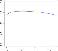
Figure 1: Proxy of the conditional likelihood of $X_{1}^{k}$ under $g_{T_{1,n}}$ as a function of $\theta$ for $n=100$ and $k=80$ in the gamma case.

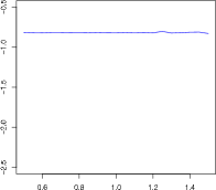
Figure 2: Proxy of the conditional likelihood of $X_{1}^{k}$ under $g_{U_{1,n}}$ as a function of $r$ for $n=100$ and $k=80$ in the gamma case.

We also consider the Inverse Gaussian distribution with density

$$f_{\lambda,\mu}(x):=\left[\frac{\lambda}{2\pi}\right]^{1/2}\exp-\frac{\lambda\left(x-\mu\right)^{2}}{2\mu^{2}x}\text{ \ \ \ for }x>0$$ (8)

with both parameters $\lambda$ and $\mu$ be positive. Given an i.i.d. sample $X_{1}^{n}:=\left(X_{1},...,X_{n}\right)$ with density $f_{\mu,\lambda}$, the resulting sufficient statistics are respectively $T_{1,n}:=X_{1}+...+X_{n}$ and $U_{1,n}:=X_{1}^{-1}+...+X_{n}^{-1}.$ Similarly as for the Gamma case we draw the likelihood of a subsample $X_{1}^{k}$ under $g_{u_{1,n}}$ with $T_{1,n}:=X_{1}+...+X_{n}$ ,which is a sufficient statistics for $\mu$ (Figure 3), and upon $U_{1,n}:=X_{1}^{-1}+...+X_{n}^{-1}$ which is sufficient for $\lambda$ (Figure 4). In either cases the other coefficient is kept fixed at the true value of the parameter generating the sample. As for the Gamma case these curves show the invariance of the proxy of the conditional density with respect to the parameter for which the chosen statistics is sufficient.

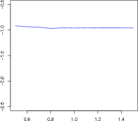
Figure 3: Conditional likelihood of $X_{1}^{k}$ under $g_{T_{1,n}}$ as a function of $\mu$ for $n=100$ and $k=80$ in the Inverse Gaussian case.

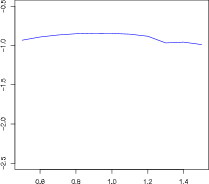
Figure 4: Conditional likelihood of $X_{1}^{k}$ under $g_{U_{1,n}}$ as a function of $\lambda$ for $n=100$ and $k=80$ in the Inverse Gaussian case.

3.2 Rao-Blackwellisation

Rao-Blackwell Theorem holds regardless of whether biased or unbiased estimators are used, since it reduces the MSE. Although its statement is rather weak, in practice, however, the improvement is often enormous. New interest in Rao-Blackwellisation procedures have risen in the recent years, conditioning on ancillary variables (see Fraser(2004) [13] for a survey on ancillaries in conditional inference); specific Rao-Blackwellisation schemes have been proposed by Casella and Robert [6], [7], Perron(1999)[26], Douc and Robert (2010)[28] and Iacobucci et all.(2010) [14]. The purpose is to improve the variance of a given statistics (for example a tail probability) under a known distribution, through a simulation scheme under this distribution; the ancillary variables used in the simulation process itself are used as conditioning ones for the Rao-Blackwellisation of the statistics. The present approach is more classical in this respect, since we do not assume that the parent distribution is known; conditioning on a sufficient statistics $\mathbf{U}_{1,n}$ with respect to the parameter $\theta$ and simulating samples according to the approximating density $g_{u_{1,n}}$ will produce the improved estimator.

Since $U_{1,n}$ is sufficient for the parameter $\theta$ in $g_{u_{1,n}}$ it can be used in order to obtain improved estimators of $\theta_{T}$ through Rao Blackwellization. We shortly illustrate the procedure and its results on some toy cases. Consider again the Gamma family defined here-above with canonical parameters $r$ and $\theta$.

First the parameter to be estimated is $\theta_{T}.$ A first unbiaised estimator is chosen as

$$\widehat{\theta}_{2}:=\frac{X_{1}+X_{2}}{2r_{T}}.$$

Given an i.i.d. sample $X_{1}^{n}$ with density $\gamma_{r_{T},\theta_{T}}$ the Rao-Blackwellised estimator of $\widehat{\theta}$ is defined through

$$\theta_{RB,2}:=E\left(\left.\widehat{\theta_{2}}\right|U_{1,n}\right)$$

whose variance is less than $Var\widehat{\theta_{2}}.$

Consider $k=2$ in $g_{U_{1,n}}(y_{1}^{k})$ and let $\left(Y_{1},Y_{2}\right)$ be distributed according to $g_{u_{1,n}}(y_{1}^{2}).$ Replications of $\left(Y_{1},Y_{2}\right)$ induce an estimator of $\theta_{RB,2}$ for fixed $u_{1,n}.$ Iterating on the simulation of the runs $X_{1}^{n}$ produces, for $n=100$ an i.i.d. sample of $\theta_{RB,2}$’s and the $Var\theta_{RB,2}$ is estimated. The resulting variance shows a net improvement with respect to the estimated variance of $\widehat{\theta}_{2}.$ It is of some interest to confront this gain in variance as the number of terms involved in $\widehat{\theta}_{k}$ increases together with $k.$ As $k$ approaches $n$ the variance of $\widehat{\theta}_{k}$ approaches the Cramer Rao bound. The graph below shows the decay in variance of $\widehat{\theta}_{k}.$ We note that whatever the value of $k$ the estimated value of the variance of $\theta_{RB,k}$ is constant. This is indeed an illustration of Lehmann-Scheffé’s theorem.

Figure 5: Variance of $\widehat{\theta}_{k}$, the initial estimator (dotted line), along with the variance of $\theta_{RB,k}$, the Rao-Blackwellised estimator (solid line) with $n=100$ as a function ok $k.$

Remark 4

Lockhart and O’Reilly (2005) [19] establish, under certain conditions and for fixed $k,$ the asymptotic equivalence of the plug-in estimate for the distribution $P_{\theta_{ML}}\left(\mathbf{X}_{1}^{k}\in B\right)$ and the Rao-Blackwell estimate $P\left(\left.\mathbf{X}_{1}^{k}\in B\right|\mathbf{U}_{1,n}\right)$ where $\theta_{ML}$ is the maximum likelihood estimator of $\theta_{T}$ based on the whole sample $\mathbf{X}_{1}^{n}$ (this result is known as Moore’s conjecture (see Moore(1973)[23])). They also provide rates for this convergence.

4 Exponential models with nuisance parameters

4.1 Conditional inference in exponential families

We consider the case when the parameter consists in two distinct subparameters, one of interest denoted $\theta$ and a nuisance component denoted $\eta$. As is well known, conditioning on a sufficient statistics for the nuisance parameter produces a new exponential family which is free of it. Assuming the observed dataset $\mathbf{x}_{1}^{n}:=\left(\mathbf{x}_{1},...,\mathbf{x}_{n}\right)$ resulting from sampling of a vector $\mathbf{X}_{1}^{n}:=\left(\mathbf{X}_{1},...,\mathbf{X}_{n}\right)$ of i.i.d. random variables with distribution in the initial exponential model, and denoting $u\left(\mathbf{x}_{1}^{n}\right)$ a sufficient statistics for $\eta,$ simulation of samples under the conditional distribution of $\mathbf{X}_{1}^{n}$ given $u\left(\mathbf{X}_{1}^{n}\right)=$ $u\left(\mathbf{x}_{1}^{n}\right)$ and $\theta=\theta_{0}$ for some $\theta_{0}$ produces the basic ingredient for Monte Carlo tests with $H_{0}:\theta_{T}=\theta_{0}$ where $\theta_{T}$ stands for the true value of the parameter of interest. Changing $\theta_{0}$ for other values of the parameter of interest produces power curves as functions of the level of the test. This is the well known principle of Monte Carlo tests, and such is the goal of the present section. We consider a steep but not necessarily regular exponential family exponential family $\mathcal{P}:=\{P_{\theta,\eta},(\theta,\eta)\in\mathcal{N}\}$ defined on $\mathbb{R}$ with canonical parametrization $(\theta,\eta)$ and minimal sufficient statistics $\left(t,u\right)$ defined on $\mathbb{R}$ through the density

$$p_{\theta,\eta}(x):=\frac{dP_{\theta,\eta}\left(x\right)}{dx}=\exp\left[\theta t(x)+\eta u(x)-K(\theta,\eta)\right]h(x).$$ (9)

For notational conveniency and without loss of generality both $\theta$ and $\eta$ belong to $\mathbb{R}$. Also the model can be defined on $\mathbb{R}^{d}$, $d>1$, at the cost of similar but more envolved tools. The natural parameter space is $\mathcal{N}$ (which is a convex set in $\mathbb{R}^{2}$) defined as the effective domain of

$$k(\theta,\eta):=\exp\left[K(\theta,\eta)\right]=\int\exp\left[\theta t(x)+\eta u(x)\right]h(x)dx.$$ (10)

Let $X_{1}^{n}:=\left(X_{1},...,X_{n}\right)$ be $n$ i.i.d. replications of a general random variable $\mathbf{X}$ with density (9). Denote

$$T_{1,n}:=\sum_{i=1}^{n}t(X_{i})\mathit{\ \ }\text{and}\mathit{\ \ \ }U_{1,n}:=\sum_{i=1}^{n}u(X_{i}).$$ (11)

Basu (1977) [3] discusses ten different ways for eliminating the nuisance parameters, among which conditioning on sufficient statistics and consider UMPU tests pertaining to the parameter of interest. In most cases, the density of $T_{1,n}$ given $U_{1,n}=u_{1,n}$ is unknown. Two main ways have been developped to deal with this issue: approximating this conditional density of a statistics or simulating samples from the conditional density. We compose these two approaches in the present paper.

The classical technique is to approximate this conditional density using some expansion. Then integration produces critical values. For example, Pedersen (1979) [24] states the mixed Edgeworth-saddlepoint approximation, or the single saddlepoint approximation. However, the main issue of this technique is that the approximated density still depends on the nuisance parameter. In order to obtain the expansion, some suitable values for the parameter of interest and for the nuisance parameter have to be chosen. In the method developped here, as seen before, the conditional approximated density inherits of the invariance with respect to the nuisance parameter when conditioning on a sufficient statistics pertaining to this parameter.

Rephrasing the notation of Section 2 in the present setting it holds that the MLE $\left(\theta_{ML},\eta_{ML}\right)$ satisfies

$$\left.\frac{\partial K\left(\theta,\eta\right)}{\partial\eta}\right|_{\theta_{ML},\eta_{ML}}=u_{1,n}/n$$

and therefore $u_{1,n}/n$ converges to $\left(\frac{\partial K\left(\theta_{T},\eta\right)}{\partial\eta}\right)^{-1}\left(\eta_{T}\right).$

For notational clearness denote $\mu$ the expectation of $u\left(\mathbf{X}_{1}\right)$ and $\sigma^{2}$ its variance under $\left(\theta_{T},\eta_{T}\right)$ , hence

$$\mu:=\mu_{\left(\theta_{T},\eta_{T}\right)}:=\partial K(\theta_{T},\eta_{T})/\partial\eta\text{ \ \ \ \ }\sigma^{2}:=\sigma_{\left(\theta_{T},\eta_{T}\right)}^{2}:=\partial^{2}K(\theta_{T},\eta_{T})/\partial\eta^{2}\text{ }$$

Assume at present $\theta_{T}$ and $\eta_{T}$ known. It holds

$$\phi(r) :=E_{\left(\theta_{T},\eta_{T}\right)}\exp[ru\left(\mathbf{X}\right)]=\exp\left[K(\theta_{T},\eta_{T}+r)-K(\theta_{T},\eta_{T})\right]$$

and

$$m(r) =\mu_{\left(\theta_{T},\eta_{T}+r\right)}$$

$$s^{2}(r) =\sigma_{\left(\theta_{T},\eta_{T}+r\right)}^{2}$$

$$\mu_{3}(r) =\partial^{3}K(\theta_{T},\eta_{T}+r)/\partial\eta^{3}\text{ .}$$

Further

$$\pi_{u,\theta_{T},\eta_{T}}^{\alpha}(x):=\frac{\exp ru(x)}{\phi(r)}p_{\left(\theta_{T},\eta_{T}\right)}\left(x\right)=p_{\left(\theta_{T},\eta_{T}+r\right)}\left(x\right)$$ (12)

for any given $\alpha$ in the range of $P_{\theta_{T},\eta_{T}}.$ In the above formula (12) the parameter $r$ denotes the only solution of the equation

$$m(r)=\alpha.$$

For large $k$ depending on $n,$ using Monte Carlo tests based on runs of length $k$ instead of $n$ does not affect the accuracy of the results.

4.2 Application of conditional sampling to MC tests

Consider a test defined through $H_{0}:\theta_{T}=\theta_{0}$ versus $H_{1}:\theta_{T}\neq\theta_{0}$ Monte Carlo (MC) tests aim at obtaining $p-$values through simulation. where the distribution of the desired test statistics under $H_{0}$ is either unknown or very cumbersome to obtain; a comprehensive reference is Jöckel(1986), [15].

Recall the principle of thoses tests: denote $t$ the observed value of the studied statistic based on the dataset and let $t_{2},..,t_{L}$ the values of the resulting test statistics obtained through the simulation of $L-1$ samples $\mathbf{X}_{1}^{n}$ under $H_{0}.$ If $t$ is the $M$th largest value of the sample $(t,t_{2},...,t_{L})$, $H_{0}$ will be rejected at the $\alpha=M/L$ signifiance level, since the rank of $t$ is uniformly distributed on the integer $2,...,L$ when $H_{0}$ holds. Calculation of power functions can be handled similarly. The above approximation of the conditional density $p_{u_{1,n}}\left(x_{1}^{k}\right)$ involves the unknown parameters $\theta_{T}$ and $\eta_{T}$ in all the simulation steps. This problem is solved when simulating under $H_{0}:\theta_{T}=\theta_{0}$ setting $\theta_{0}$ in place of $\theta_{T}$ and $\hat{\eta}_{\theta_{0}}$ in place of $\eta_{T}$, where $\hat{\eta}_{\theta_{0}}$ is the MLE of $\eta_{T}$ in the one parameter family $p_{\theta_{0},\eta}$ defined through (9). This choice follows the commonly used one, as advocated for instance in [24] and [25]. Innumerous simulation studies support this choice in various contexts.

Consider the problem of testing the null hypothesis $H_{0}:\theta_{T}=\theta_{0}$ against the alternative $H_{1}:\theta_{T}>\theta_{0}$ in model (10) where $\eta$ is the nuisance parameter.

When $p_{u_{1,n},\theta_{0}}$ is known, the classical conditional test $H_{0}:\theta_{T}=\theta_{0}$ versus $H_{1}:\theta_{T}>\theta_{0}$ with level $\alpha$ is UMPU.

Substituting $p_{\theta_{0}}\left(\mathbf{X}_{1}^{n}=x_{1}^{n}\left|\mathbf{U}_{1,n}=u_{1,n}\right.\right)$ by $g_{u_{1,n},\theta_{0}}\left(x_{1}^{k}\right)$ defined in (6), i.e. substituting the test statistics $T_{1}^{n}$ by $T_{1}^{k}$ and $p_{\theta_{0}}\left(\mathbf{X}_{1}^{k}=x_{1}^{k}\left|\mathbf{U}_{1,n}=u_{1,n}\right.\right)$ by $g_{u_{1,n},\theta_{0}}\left(x_{1}^{k}\right)$ i.e. changing the model for a proxy while keeping the same parameter of interest $\theta$ yields the conditional test with level $\alpha$

$$\psi_{\alpha}(x_{1}^{k}):=\left\{\begin{array}[]{r}1\text{\ \ if\ \ }T_{1,k}>t_{\alpha}\\ \gamma\text{\ \ if\ \ }T_{1,k}=t_{\alpha}\\ 0\text{\ \ if\ \ }T_{1,k}<t_{\alpha}\end{array}\right.$$

and

$$E_{G_{u_{1,n}}}[\psi_{\alpha}(X_{1}^{k})]=\alpha$$

i.e. $\alpha:=\int\mathds{1}_{t_{1,k}>t_{\alpha}}g_{u_{1,n}}\left(x_{1}^{k}\right)dx_{1}...dx_{k}.$ Its power under a simple hypothesis $\theta_{T}=\theta$ is defined through

$$\beta_{\psi_{\alpha}}(\theta|u_{n})=E_{\theta}[\psi_{n}(T_{1,n},U_{1,n})|U_{1,n}=u_{1,n}].$$

Recall that the parametric bootstrap produces samples from a parametric model which is fitted to the data, often through maximum likelihood. In the present setting, the parameter $\theta$ is set to $\theta_{0}$ and the nuisance parameter $\eta$ is replaced by its estimator $\widehat{\eta}_{\theta_{0}}$ which is the MLE of $\eta$ when the parameter $\theta$ is fixed at the value $\theta_{0}$ defining $H_{0}.$ Comparing their exact conditional MC tests with parametric bootstrap ones for Gamma distributions, Lockhart et al(2007)[19] conclude that no significant difference can be notices in terms of level or in terms of power. We proceed in the same vein, comparing conditional sampling MC tests with the parametric bootstrap ones, obtaining again similar results when the nuisance parameter is estimated accurately. However the results are somehow different when the nuisance parameter cannot be estimated accurately, which may occur in various cases.

In practice since the chosen conditioning statistics is quasi sufficient for the nuisance parameter, we plug any value for this parameter in the definition of $g_{u_{1,n}}.$ This is what has been performed in all examples below.

4.3 Unimodal Likelihood: testing the coefficients of a Gamma distribution

Let $\mathbf{X}_{1}^{n}$ be an i.i.d. sample of random variables with Gamma distribution $\Gamma\left(a_{T},b_{T}\right)$ where $a_{T}$ is the shape coefficient and $b_{T}$ is the scale coefficient. As $a$ and $b$ vary this distribution is a two parameter exponential family. The statistics $T_{1,n}:=\mathbf{X}_{1}+...+\mathbf{X}_{n}$ is sufficient for the parameter $a$ and $U_{1,n}:=\log\mathbf{X}_{1}+...+\log\mathbf{X}_{n}$ is sufficient for $b.$

MC conditional test with $H_{0}:a_{T}=a_{0}$

Denote $u_{1,n}=\sum_{i=1}^{n}X_{i}$ and $\hat{b}_{a_{0}}$ the MLE of $b.$ Calculate for $l\in\{2,L\}$

$$t_{l}:=\sum_{i=0}^{k}\log\left(Y_{i}(l)\right).$$

where the $Y_{i}^{\prime}$ are a sample from $g_{u_{1,n}}^{a_{0},\hat{b}_{a_{0}}}.$

Consider the corresponding parametric bootstrap procedure for the same test, namely simulate $Z_{i}(l)$, $2\leq l\leq L$ and $0\leq i\leq k$ with distribution $\Gamma\left(a_{0},\hat{b}_{a_{0}}\right);$ denote

$$s_{l}:=\sum_{i=0}^{k}\log\left(Z_{i}(l)\right).$$

In this example simulation shows that for any $\alpha$ the $M$th largest value of the sample $\left(t,t_{2},...,t_{L}\right)$ is very close to the corresponding empirical $M/L$-quantile of $s_{l}$’s. Hence Monte Carlo tests through parametric bootstrap and conditional compete equally. Also in terms of power, irrespectively in terms of $\alpha$ and in terms of alternatives (close to $H0$), the two methods seem to be equivalent.

MC conditional test with $H_{0}:b_{T}=b_{0}$

Denote $u_{1,n}=\sum_{i=1}^{n}\log\left(X_{i}\right)$ and $\hat{a}_{b_{0}}$ the MLE of $a.$ Calculate for $l\in\{2,L\}$

$$t_{l}:=\sum_{i=0}^{k}Y_{i}(l)$$

where the $Y_{i}^{\prime}$ are a sample from $g_{u_{1,n}}^{b_{0},\hat{a}_{b_{0}}}$ and, as above define accordingly

$$s_{l}:=\sum_{i=0}^{k}\log\left(Z_{i}(l)\right)$$

where the $Z_{i}(l)$’s are simulated under $\Gamma\left(\hat{a}_{b_{0}},b_{0}\right).$

As above, parametric bootstrap and conditional sampling yield equivalent Monte Carlo tests in terms of power function under alternatives close to $H0$.

In the two cases studied above  the value of $k$ has been obtained through the rule exposed in section 3.2 of Broniatowski and Caron (2011) [4].

4.3.1 Bimodal likelihood: testing the mean of a normal distribution in dimension 2

In contrast with the above mentionned examples, the following case study shows that estimation through the unconditional likelihood may fail to provide consistent estimators when the likelihood surface has multiple critical points. This in turn yields parametric bootstrap Monte Carlo tests with inacceptable power functions.

Sundberg(2009)[30] proposes four examples that allow likelihood multimodality. Two of them can also be found in [9] and [10], and in [2], Ch 2. We consider the ”Normal parabola” model which is a curved (2, 1) family (see Example 2.35 in [2], Ch 2 ). Two independent Gaussian variates have unknown means and known variances; their means are related by a parabolic relationship.

Let $X$ et $Y$ be two independent gaussian r.v.’s with same variance $\sigma_{T}^{2}$ with expectation $\psi_{T}$ and $\psi_{T}^{2}$. In the present example $\sigma_{T}^{2}=1$ and $\psi_{T}=2.$

Let $\left(X_{i},Y_{i}\right)$ , $1\leq i\leq n$ be an i.i.d. sample with the above distribution.

The parameter of interest is $\sigma^{2}$ whislt the nuisance parameters is $\psi.$ Derivation of the likelihood function of the observed sample with respect to $\psi$ yields the following equation

$$\left(U_{1,n}-\psi\right)+2\psi\left(V_{1,n}-\psi^{2}\right)=0$$

with $U_{1,n}:=X_{1}+...+X_{n}$ and $V_{1,n}:=Y_{1}+...+Y_{n}.\$The following table shows that the likelihood function is bimodal in $\psi.$

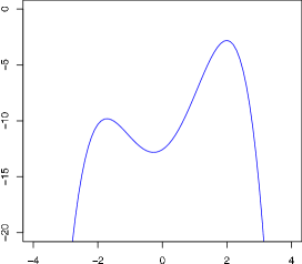
Figure 6: Bimodal likelihood in $\psi.$

Estimation of the nuisance parameter $\psi$ is performed through the standard Newton Raphson method. The Newton-Raphson optimizer of the likelihood function converges to the true value when the initial value is larger than 1and fails to converge to $\psi_{T}=2$ otherwise. Hencefore the parametric bootstrap estimation of the likelihood function of the sample based on this preliminary estimate of the nuisance parameter may lead to erroneous estimates of the parameter of interest. Indeed  according to the initial value we obtained estimators of $\psi_{T}$ close to $2$ or to $-2.$ When the estimator of the nuisance parameter is close to its true value $2$ then parametric bootstrap yields Monte Carlo tests with power close to $1$ for any $\alpha$ and any alternative close to $H0.$ At the contrary when this estimate is close to the second maximizer of the likelihood (i.e. close to $-2$) then the resulting Monte Carlo test based on parametric bootstrap has power close to $0$ irrespectively of the value of $\alpha$ and of the alternative, when close to $H0.$ In contrast with these results, Monte Carlo tests based on conditional sampling provide powers close to $1$ for any $\alpha$; we have considered alternatives close to $H0$ . This result is of course a consequence of quasi sufficiency of the statistics $\left(U_{1,n},V_{1,n}\right)$ for the parameter $\psi$ of the distribution of the sample $\left(X_{i},Y_{i}\right)_{i=1,...,n}$; see next paragraph for a discussion of this point.

4.4 Estimation through conditional likelihood

Considering model (10) we intend to perform an estimation of $\theta_{T}$ irrespectively upon the value of $\eta_{T}$. Denote $\widehat{\eta}_{\theta}$ the MLE of $\eta_{T}$ when $\theta$ holds; the model $p_{\theta,\widehat{\eta}_{\theta}}(x)$ is a one parameter model which is fitted to the data for any peculiar choice of $\theta.$ The classic unconditional likelihood provides consistent estimators of $\theta_{T}$ in many cases. However, this method strongly relies on the constistency properties of $\widehat{\eta}_{\theta}$ at any given $\theta.$

For fixed parameter value $\theta$ of the parameter of interest, Theorem 1 means that the likelihood of the subsample $\mathbf{X}_{1}^{k}$ with unknown distribution with parameter $\left(\theta_{T},\eta_{T}\right)$ under the distribution with any parameter $\theta$ given the value of the sufficient statistics $U_{1,n}$ is approximated by $g_{u_{1,n}}\left(\mathbf{X}_{1}^{k}\right)$ when $\mathbf{X}_{1}^{k}$ is either generated under the conditional density or under $g_{u_{1,n}}$   with parameter $\eta=\eta_{T}.$ Substituting $\eta_{T}$ by its estimator should yield maximal value of the approximate likelihood when $\left(\theta_{T},\eta_{T}\right)$ holds, since $\widehat{\eta}_{\theta}$ approaches $\eta_{T}$ when $\theta=\theta_{T}.$ In particular, this holds when $\mathbf{X}_{1}^{k}$ is generated under $\theta_{T},\eta_{T}$ which holds on the observed sample. This yields to an algorithm to estimate $\theta_{T}.$ For any $\theta$ calculate $\widehat{\eta}_{\theta}$ . Evaluate $g_{u_{1,n}}\left(\mathbf{X}_{1}^{k}\right)$ and optimize in $\theta.$

In most cases, as the normal, gamma or inverse-gaussian, both estimation through the unconditional likelihood and estimation through conditional likelihood based on the proxy $g_{u_{1,n}}$ give a consistent estimator.

We consider the example of the Bimodal likelihood from the above subsection, inheriting of the notation and explore the behaviour of the proxy of the conditional likelihood of the sample $\left(X_{i},Y_{i}\right)$ , $1\leq i\leq n$ when conditioning on $U_{1,n}$ and $V_{1,n}$ , as a function of $\sigma^{2}.$ The likelihood writes

$$L\left(\left.\sigma^{2}\right|\left(X_{i},Y_{i}\right),1\leq i\leq n,U_{1,n},V_{1,n}\right)$$

$$=P_{\mathbf{X}_{1}^{n}}\left(\left.X_{1}^{n}\right|U_{1,n},\sigma^{2}\right)P_{\mathbf{Y}_{1}^{n}}\left(\left.Y_{1}^{n}\right|V_{1,n},\sigma^{2}\right)$$

where we have used the independence of the r.v.’s $X_{i}$’s and $Y_{i}$’s.

Applying Theorem 1 to the above expression it appears that $\psi$ cancels in the resulting density $g_{u_{1,n}}$ and $g_{v_{1,n}}.$ This proves that the proxy of the conditional likelihood provides consistent estimation of $\sigma_{T}^{2}$ as shown on Figures 7 and 8 (see the solid lines).

On Figure 7, the dot line is the empirical likelihood function with consistent estimator of the nuisance parameter; the resulting maximizer in the variable $\sigma^{2}$ is close to $\sigma_{T}^{2}=1.$ At the opposite in Figure 8 an inconsistent preliminary estimator of $\psi_{T}$ obtained through a bad tuning of the initial point in the Newton-Raphson procedure leads to unconsistency in the estimation of $\sigma_{T}^{2}$, the resulting likelihood function being unbounded.

Figure 7: Proxy of the conditional likelihood (solid line) along with the empirical likelihood (dotted line) as function of $\sigma^{2}$ for $n=100$ and $k=99$ in the case where a good initial point in Newton-Raphson procedure is chosen.

Figure 8: Proxy of the conditional likelihood (solid line) along with the empirical likelihood (dotted line) as function of $\sigma^{2}$ for $n=100$ and $k=99$ in the case where a bad initial point in Newton-Raphson procedure is chosen.

References

- [1] Barndorff-Nielsen, O.E. (1978). Information and exponential families in statistical theory. Wiley Series in Probability and Mathematical Statistics. Chichester: John Wiley & Sons.
- [2] Bardnörff-Nielsen, O.E. and Cox, R.R. (1994). Inference and Asymptotics. Chapman & Hall, London.
- [3] Basu, D. (1977). On the elimination of nuisance parameters. J. Amer. Statist. Assoc. 72 (1977), no. 358, 355–366.
- [4] Broniatowski M. and Caron, V. (2011). Long runs under point conditioning. The real case. arXiv:1010.3616v5.
- [5] Broniatowski M. and Caron, V. (2011). Towards zero variance estimators for rare event probabilities. arXiv:1104.1464v2.
- [6] Casella, G. and Robert, C. P. (1996). Rao-Blackwellisation of sampling schemes. Biometrika 83 , no. 1, 81–94.
- [7] Casella, G. and R. C. P. (1998). Post-processing accept-reject samples: recycling and rescaling. J. Comput. Graph. Statist. 7 , no. 2, 139–157
- [8] Cheng, R.C.H. (1984). Generation of inverse Gaussian variates with given sample mean and dispersion. Appl. Statist. 33, 309–16
- [9] Efron, B. (1975). Defining the curvature of a statistical problem (with applications to second order efficiency) (with discussion). Ann. Statist. 3, 1189-1242.
- [10] Efron, B. (1978). The geometry of exponential families. Ann. Statist. 6, 362-376.
- [11] Efron, B. (1979), Bootstrap methods: another look at the jackknife. Ann. Statist. 7 , no. 1, 1–26.
- [12] Engen, S. and Lillegard, M. (1997). Stochastic simulations conditioned on sufficient statistics. Biometrika, 84, 235–240.
- [13] Fraser, D. A. S. (2004). Ancillaries and conditional inference. With comments by Ronald W. Butler, Ib M. Skovgaard, Rudolf Beran and a rejoinder by the author. Statist. Sci. 19 , no. 2, 333–369
- [14] Iacobucci, A., Marin, J.-M., Robert, C. (2010). On variance stabilisation in population Monte Carlo by double Rao-Blackwellisation. Comput. Statist. Data Anal. 54 , no. 3,
- [15] Jöckel, K.-H. (1986). Finite sample properties and asymptotic efficiency of Monte Carlo tests. Ann. of Stat., 14, 336–347.
- [16] Lehmann, E.L. (1986). Testing Statistical Hypotheses. Springer.
- [17] Lindqvist, B.H., Taraldsen, G., Lillegärd, M. and Engen, S. (2003). A counterexample to a claim about stochastic simulations. Biometrika 90 , no. 2, 489–490.
- [18] Lindqvist, B.H. and Taraldsen, G. (2005). Monte Carlo conditioning on a sufficient statistic. Biometrika 92 , no. 2, 451–464.
- [19] Lockhart, R. and O’Reilly, F. (2005) A note on Moore’s conjecture. Statist. Probab. Lett. 74 , no. 2, 212–220.
- [20] Lockhart, R A., O Reilly, F J. and Stephens, A. (2007) Use of the Gibbs sampler to obtain conditional tests, with applications. Biometrika 94 , no. 4, 992–998.
- [21] Lockhart, R.A. and Stephens, M. A. (1994). Estimation and tests of fit for the three–parameter Weibull distribution. J. Roy. Statist. Soc.. B. 56:491–500.
- [22] O’Reilly, F. and Gravia-Medrano, L. (2006). On the conditional distribution of goodness-of-fit tests. Commun. Statist. A, 35:541–9.
- [23] Moore, David S. (1973). A note on Srinivasan’s goodness-of-fit test. Biometrika 60 , 209–211.
- [24] Pedersen, B.V., (1979). Approximating conditional distributions by the mixed Edgeworth-saddlepoint expansion. Biometrika, 66(3), 597–604.
- [25] Pace L. and Salvan A., (1992). A note on conditional cumulants in canonical exponential families. Scand. J. Statist., 19, 185–191.
- [26] Perron, F. (1999). Beyond accept-reject sampling. Biometrika 86 , no. 4, 803–813
- [27] Reid, N. (1995). The roles of conditioning in inference. With comments by V. P. Godambe, Bruce G. Lindsay and Bing Li, Peter McCullagh, George Casella, Thomas J. DiCiccio and Martin T. Wells, A. P. Dawid and C. Goutis and Thomas Severini. With a rejoinder by the author. Statist. Sci. 10 , no. 2, 138–157, 173–189, 193–196.
- [28] Douc, R. and Robert, C.P.(2011). A vanilla Rao-Blackwellization of Metropolis-Hastings algorithms. Ann. Statist. 39 , no. 1, 261–277
- [29] Severini T.A. (1994), On the approximate elimination of nuisance parameters by conditioning. Biometrika, 81(4), 649–661.
- [30] Sundberg, R. (2009). Flat and multimodal likelihoods and model lack of fit in curved exponential families. Research Report 2009:1, http://www.math.su.se/matstat.