Self Contained Encrypted Image Folding

Abstract

The recently introduced approach for Encrypted Image Folding is generalized to make it self-contained. The goal is achieved by enlarging the folded image so as to embed all the necessary information for the image recovery. The need for extra size is somewhat compensated by considering a transformation with higher folding capacity. Numerical examples show that the size of the resulting cipher image may be significantly smaller than the plain text one. The implementation of the approach is further extended to deal also with color images.

1 Introduction

As cameras and digital scanners of very high resolution are becoming widely available, use of high resolution digital images is becoming part of everyday life. From a mathematical standpoint a digital image is a $2$D data array, say $I\in\mathbb{R}^{N_{x}\times N_{y}}$. Each data point is referred to as a pixel. For a gray level image, each pixel is represented with an intensity value $I$. For an RGB representation of a color image, each pixel consists of a color triple $(I_{R},I_{G},I_{B})$ representing the intensity of the red, green and blue components, respectively.

The array of pixels used to represent a high resolution digital image is expected to be huge. Obviously storage and transmission of this raw data is impractical. Consequently, a reduction in data dimensionality is essential. The process that creates a compact data representation is called compression. Because of the nature of its informational content compressing an image usually involves special techniques. As opposed to binary files where a single bit error may destroy the whole piece of data, some distortion is usually tolerable even when compressing high quality images. This is because the visual perception of the image is more important than the exact pixel values.

The most frequently applied image compression techniques involve transform coding which has three main steps: i)Application of an invertible transform to the intensity image. ii)Quantization of the transformed data. iii)Bit-stream coding.

The familiar compression standard JPEG, for instance, implements step i) using the Discrete Cosine Transform (DCT), while the more recent, JPEG2000, uses Discrete Wavelet Transform (DWT).

Another problem associated with the transmission of digital images is security. It comprises several aspects, including confidentiality and access control which are addressed by encryption. This implies that only parties holding decryption keys can access content of an image. Conventional image encryption is based on techniques developed for general data [1, 2]. In principle generic encryption can be applied to a digital image before or after compression. However, encryption before compression would change the statistical properties of the image preventing compression from being applied successfully.

On the other hand, as well as effecting the compression performance, direct encryption of the compressed data results in a bit stream that is incompatible with the original image file format. Less stringent schemes involve partial (or selective) encryption [1, 2]. However the security of these encryption systems is lower when compared to full encryption.

Enhancing security of conventional compression/encryption techniques, using a chaotic map at the bit-stream coding step, is proposed in [3, 4]. However, for the most part, the line of research for image encryption based on Chaotic Cryptography [5, 6, 7, 8, 9, 10, 11, 12, 13, 14, 15] has been developed to operate directly on the pixel$/$intensity representation of an image. An interesting critical analysis of the research in this area can be found in [16]. The connection between chaotic and conventional cryptography is considered in [17].

Chaos based image encryption takes advantage of the extreme sensitivity to initial conditions of some dynamical systems, to control the ‘confusion’ of pixels in an intensity image.

Thus, a chaotic method breaks the structure of the plain text image, producing a cipher image which is no longer compressible by conventional transform coding techniques. Hence, within the traditional chaos based framework for image encryption the problem of storage and transmission of large images is currently unsolved.

An alternative framework, involving only mathematical operations on an intensity image, but addressing simultaneously the problems of data reduction and encryption, has been recently introduced in [18]. The scheme is termed Encrypted Image Folding (EIF). The first step of this new scheme differs from step i) in the above mentioned conventional compression scheme in that, instead of using orthogonal transformations (e.g. DCT or DWT) the transformation is realized by means of highly nonlinear approximation techniques. This increases the difficulty of the approximation process but at the same time renders significant improvement in the sparsity of the image representation.

Quantization and data reduction are achieved simultaneously by embedding some of the transformed data into a section of the image. Privacy is protected by granting access to the embedded data only to key holders.

The underlying principle of the proposed framework is very simple: Suppose that an image is given as an intensity array $I\in\mathbb{R}^{N_{x}\times N_{y}}$ and suppose also that, through a transformation $\hat{B}:\mathbb{R}^{N_{x}\times N_{y}}\to\mathbb{R}^{K}$, one can approximate equivalent information from an array $c\in\mathbb{R}^{K}$ obtained as $c=\hat{B}I$. If $K<N_{x}N_{y}$ by a considerable amount, $c$ is said to be a sparse representation of the image $I$. It follows then that a suitable transformation to achieve sparsity should be rank deficient, with an associated null space, $\operatorname*{null}(\hat{B})$, of large dimensionality. Such a transformation creates room for storing covert information. Indeed, if one considers an element $F\in\operatorname*{null}(\hat{B})$ and adds it to the image, so as to create a new array $G=I+F$, one obtains the identical representation $\hat{B}G=\hat{B}I=c$. The sparser the representation of an image, the larger the null space of the associated transformation. Consequently, the first part of this effort focuses on the design of an effective transformation for this purpose. The transformation is adaptively constructed by the greedy selection strategy called Orthogonal Matching Pursuit (OMP).

The viability of EIF, as proposed in [18], stems from the possibility of processing a large image by dividing it into small blocks. This allows the representation of some of the blocks to be embedded into other blocks, realizing in that manner the folding of the image. However, the technique in [18] is not self-contained, because, in addition to the folded image, extra information is required at the unfolding step, and that information depends on the image. In this Communication we propose to extend EIF so as to make it self-contained. We term such an extension Self-Contained Encrypted Image Folding (SCEIF), because all that is needed to successfully unfold the image is the private key. This goal is accomplished by enlarging the folded image to create further space for the required information. The need for extra size is compensated by considering a transformation with the capability of yielding sparser representations than that in [18], therefore improving folding capacity. Access control to the folded image is realized using a simple symmetric key encryption algorithm. The whole procedure is characterized by its potential for real time implementation using parallel processing, but also for its competitiveness using sequential processing.

The paper is organized as follows. In Sec. 2 we discuss the strategy for achieving a high level of sparsity in image representation using the greedy selection strategy OMP, implemented here in $2$D with separable dictionaries. The framework for extending EIF to SCEIF is discussed in Sec. 3 and illustrated in Sec. 4 by its application on i) an astronomical image created at the European Southern Observatory and ii) a photograph of the natural world provided by National Geographic. Remarks on the quality and security of the recovered images are given in Sec. 5. Conclusions and final remarks and are summarized in Sec. 6.

2 Sparse Image Representation

The approach to be introduced in the next section relies on the ability to design a specific transformation which gives rise to a sparse representation of an image. This section is dedicated to the construction of such a transformation.

Suppose that an image, given as an array $I\in\mathbb{R}^{N_{x}\times N_{y}}$ of intensity pixels, is to be approximated by the linear decomposition

$$I^{K}=\sum_{k=1}^{K}c_{k}d_{\ell_{k}},$$ (1)

where each $c_{k}$ is a scalar and each $d_{\ell_{k}}$ is an element of $\mathbb{R}^{N_{x}\times N_{y}}$ to be selected from a set, $\mathcal{D}=\{d_{n}\}_{n=1}^{M}$, called a ‘dictionary’.

A sparse approximation of $I\in\mathbb{R}^{N_{x}\times N_{y}}$ is an approximation of the form (1) such that the number $K$ of elements in the decomposition is significantly smaller than ${N=N_{x}N_{y}}$. Clearly one of the crucial issues to achieve high levels of sparsity is the selection of the right elements to decompose the image. This goal has motivated the introduction of highly nonlinear techniques for image approximation, which operate outside the traditional basis framework. Instead, the terms in the decomposition are taken from a large redundant dictionary, from where the elements $d_{\ell_{k}}$ in (1), called ‘atoms’, are chosen according to some optimality criterion.

Within the redundant dictionary framework for approximation, the problem of finding the sparsest decomposition of a given image can be formulated as follows:

Approximate the image by the ‘atomic decomposition’ (1) such that the number $K$ of atoms is minimum.

Equivalently, for a dictionary of $M>N$ elements the statement is reworded as:

Find the atomic decomposition:

$$I^{K}=\sum_{n=1}^{M}c_{n}d_{n},$$ (2)

such that the counting measure $\|\mathbf{c}\|_{\alpha=0}:=\sum_{n=1}^{M}(c_{n})^{0}$ is minimized.

Unfortunately the numerical minimization of $\|\mathbf{c}\|_{\alpha=0}$ restricted to (2) involves a combinatorial problem for exhaustive search and is therefore intractable with classical means. Hence, one is forced to abandon the sparsest solution and look for a ‘satisfactory solution’, i.e, a solution such that the number of nonzero coefficients in (2) (equivalently, the number of $K$-terms in (1)) is considerably smaller than the image dimension. One possibility for constructing a solution of this nature could be to fix a value of $\alpha\in(0,1]$ and minimize the diversity measure, $\sum_{k=1}^{M}|c_{k}|^{\alpha}$ [21], closely related to the $\alpha$-entropy giving rise to the non-extensive statistical mechanics [22, 23]. However, the numerical implementation of this possibility is too demanding to apply in the present context. In contrast, the goal of finding a sparse solution can be achieved at speeds comparable to fast transforms by the greedy technique called OMP that we dedicate to be applied in $2$D. This approach selects the atoms in the decomposition (1) in a stepwise manner, as will be described in the next section.

2.1 Orthogonal Matching Pursuit in $2$D

OMP was introduced in [24]. We describe here our implementation in $2$D, henceforth referred to as OMP2D. Our version of the algorithm is specific to separable dictionaries, i.e, a $2$D dictionary which corresponds in effect to the tensor product of two $1$D dictionaries. The implementation is based on adaptive biorthogonalization and Gram-Schmidt orthogonalization procedures, as proposed in [25, 26]. However, the optimized selection proposed in [25] is not considered here, due to the computational demands of such a selection process.

The images we are concerned with are assumed to be either gray level intensity images or color images stored in a standard RGB format. This format stores three color values, R(Red), G(Green) and B(Blue), for each pixel. Hence, the color image is given as three independent $2$D arrays, each called a ‘channel’. We represent the RGB channels as the arrays $I_{z}\in\mathbb{R}^{N_{x}\times N_{y}},\,z=1,2,3$ (a gray level intensity image can be considered a particular case of this representation corresponding to a unique index $z=1$).

Given an RGB image $I_{z}\in\mathbb{R}^{N_{x}\times N_{y}},\,z=1,2,3$ and two $1$D dictionaries $\mathcal{D}^{x}=\{{D}^{x}_{n}\in\mathbb{R}^{N_{x}}\}_{n=1}^{M_{x}}$ and $\mathcal{D}^{y}=\{{D}^{y}_{m}\in\mathbb{R}^{N_{y}}\}_{m=1}^{M_{y}}$ our purpose is to approximate the arrays $I_{z}\in\mathbb{R}^{N_{x}\times N_{y}},\,z=1,2,3$ using common atoms for the three images. More precisely, for $i=1,\ldots,N_{x}$ and $j=i,\ldots,N_{y}$ we look for approximations of the form

$$I_{z}^{K}(i,j)=\sum_{n=1}^{K}c_{n}^{z}{D}^{x}_{\ell^{x}_{n}}(i){D}^{y}_{\ell^{y}_{n}}(j),\quad z=1,2,3.$$ (3)

Notice that, while the coefficients $c_{n}^{z}$ in the above decomposition depend on the image $I_{z}$, the atoms participating in the decompositions are common to all the channels. For selecting those atoms we adopt the OMP selection criterion extended to simultaneous decomposition of signals. A discussion of this criterion can be found in [27], an in our context is implemented as follows:

On setting $R_{z}^{0}=I_{z},\,z=1,2,3$ at iteration $k+1$ the algorithm selects the atoms ${D}^{x}_{\ell^{x}_{k+1}}\in\mathcal{D}^{x}$ and ${D}^{y}_{\ell^{y}_{k+1}}\in\mathcal{D}^{y}$ that maximize the sum over $z$ of the Frobenius inner products absolute value $|\langle{D}^{x}_{n},R_{z}^{k}{D}^{y}_{m}\rangle_{\mathrm{F}}|,\,n=1,\ldots,M_{x},\,m=1,\ldots,M_{y},$ i.e.,

$$\begin{split}{\ell^{x}_{k+1},\ell^{y}_{k+1}}&=\operatorname*{arg\,max}_{\begin{subarray}{c}n=1,\ldots,M_{x}\\ m=1,\ldots,M_{y}\end{subarray}}\sum_{z=1}^{3}|\sum_{\begin{subarray}{c}i=1\\ j=1\end{subarray}}^{{N_{x},N_{y}}}{D}^{x}_{n}(i)R_{z}^{k}(i,j){D}^{y}_{m}(j)|,\\ \text{with}\\ R_{z}^{k}(i,j)&=I_{z}(i,j)-\sum_{n=1}^{k}c^{z}_{n}{D}^{x}_{\ell^{x}_{n}}(i){D}^{y}_{\ell^{y}_{n}}(j),\quad z=1,2,3.\end{split}$$ (4)

The three sets of coefficients $c_{n}^{z},\,n=1,\ldots,k$ involved in (4) are such that $\|R_{z}^{k}\|_{\mathrm{F}}$ is minimum for each $z$. ($\|\cdot\|_{\mathrm{F}}$ being the Frobenius norm). This is guaranteed by calculating the coefficients $c_{n}^{z},\,z=1,2,3$ as

$$c_{n}^{z}=\langle B_{n}^{k},I_{z}\rangle_{\mathrm{F}},\quad n=1,\ldots,k,$$ (5)

where matrices $B_{n}^{k},\,n=1,\ldots,k,$ are recursively constructed at each iteration step as indicated in Appendix A.

The algorithm iterates up to step, say $K$, for which, for a given $\rho$, the stopping criterion $\sum_{z=1}^{3}||I_{z}-I_{z}^{K}||^{2}_{\mathrm{F}}<\rho$ is met. The MATLAB function for the implementation of the OMP2D approach on multiple $2$D signals, which we have called OMP2DMl, is available from [28]. The corresponding MEX file in C++, for faster implementation of the identical function, is also available from [28].

2.2 Constructing the dictionary

The other crucial design for success in finding a ‘good enough’ sparse representation of the form (3) is the dictionary which provides the possible choices of atoms at the selection step.

The mixed dictionary used in [18] for this purpose consists of two components for each $1$D dictionary:

• A Redundant Discrete Cosine dictionary (RDC) $\mathcal{D}^{x}_{1}$ as given by:

  $$\mathcal{D}^{x}_{1}=\{w^{c}_{i}\cos(\frac{\pi(2j-1)(i-1)}{2M_{x}}),\,j=1,\ldots,N_{x}\}_{i=1}^{M_{x}},$$

  with $w^{c}_{i},\,i=1,\ldots,M_{x}$ normalization factors. For $M_{x}=N_{x}$ this set is a Discrete Cosine orthonormal basis for the Euclidean space $\mathbb{R}^{N_{x}}$. For $M_{x}=2lN_{x}$, with $l\in\mathbb{N}$, the set is an RDC dictionary with redundancy $2l$, that will be fixed equal to 2.

• The standard Euclidean basis, also called the Dirac basis, i.e.

  $$\mathcal{D}^{x}_{2}=\{e_{i}(j)=\delta_{i,j},\,j=1,\ldots,N_{x}\}_{i=1}^{N_{x}}.$$

Now we include an additional component:

• A family of cubic B-spline dictionaries of different support, as proposed in [29], but discretizing the domain by taking the value of a prototype B-spline only at the knots and translating that prototype one point at each translation step. Each B-spline based dictionary is given as

  $$\mathcal{D}^{x}_{s}=\{w^{s}_{i}B^{s}_{m}(j-i)|N_{x};j=1,\ldots,N_{x}\}_{i=1}^{M_{x}^{s}},$$

  where the notation $B^{s}_{m}(j-i)|N_{x}$ indicates the restriction of the B-spline of order $m$, centered at the point $i$, to be an array of size $N_{x}$. Cubic splines are obtained setting $m=4$. The factors $w^{s}_{i},\,i=1,\ldots,{M_{x}}^{s}$ are normalization constants, with $M_{x}^{s}$ the number of atoms in the dictionary $s$. The values of $s$ to be considered are $s=3$ and $s=4$, which label the dictionaries arising as translation of a prototype B-spline having, respectively, 3 and 7 points of nonzero value (see Fig. 1).

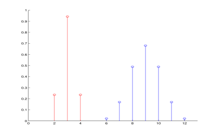
Figure 1: The discrete prototype cubic B-splines of supports 3, and 7, generating (by translation at every point) the dictionaries $\mathcal{D}^{x}_{3}$ and $\mathcal{D}^{x}_{4}$, respectively.

The complete $1$D dictionary is constructed as $\mathcal{D}^{x}=\cup_{s=1}^{4}\mathcal{D}^{x}_{s}$. The dictionary $\mathcal{D}^{y}$ is built in equivalent fashion, but changing $N_{x}$ to $N_{y}$ and $M_{x}$ to $M_{y}$ when applicable.

The required $2$D dictionary is formed as $\mathcal{D}=\mathcal{D}^{x}\otimes\mathcal{D}^{y}$. However, it is not necessary to store the $2$D dictionary $\mathcal{D}$, since the algorithm takes advantage of the separability inherent in its construction. This advantage significantly reduces storage demands and extends the possibility of using the OMP approach in $2$D.

It is time now to examine closely the term ‘good enough’ for a sparse decomposition. Within the present context by the term good enough we mean a decomposition that a)increases sparsity well beyond the levels attained by such techniques as DCT or DWT, and b)requires comparable computational time.

Remark 1.

The suitability of the mixed dictionary for block processing is essential in fulfilling requirements a) and b) above, i.e., for processing an image by dividing it into small blocks and approximate the blocks independently. This feature renders the complexity of the highly nonlinear, and otherwise costly selection technique, linear in terms of the number of blocks employed in decomposing the image.

The capacity of the dictionary based approach to achieve a satisfactory sparse approximation of an image will become clear when illustrating the SCEIF technique in Sec. 4. In addition, we present some comparisons on the results on standard test images which are listed in the first column of Table 1. All the images are 8-bit gray level intensity images of $512\times 512$ pixels. For the actual processing we divide each image into blocks of $8\times 8$ pixels and process the blocks independently. The approximated blocks are then assembled to give the approximated image.

Image	Dictionary	DCT	DWT
Barbara	5.02	3.10	2.94
Boat	4.61	2.61	2.60
Bridge	3.24	1.79	1.86
Film Clip	5.86	3.29	3.34
Lena	6.51	3.81	4.04
Mandrill	2.85	1.64	1.64
Peppers	5.23	2.88	2.96

Table 1: Comparison of the Sparsity Ratio (for PSNR $43$dB ) achieved by the mixed dictionary (second column) and that yielded by DCT and DWT (3rd and 4th columns respectively). The first column lists the names of the popular test images where the approaches are compared.

Sparsity is measured by the Sparsity Ratio (SR) defined as

$${\text{SR}}=\frac{\text{total number of pixels}}{\text{total number of coefficients}}.$$

In all the cases the number of coefficients is determined as the one required to produce a high quality approximation with no visual deterioration with respect to the original image, in this case corresponding to a PSNR of $43$dB (c.f. (16)). The sparsity results achieved by selecting atoms with OMP2D, from the proposed mixed dictionary, are displayed in the second column of Table 1. The third column shows results produced by the DCT implemented using the same blocking scheme. For further comparison the results produced by the Cohen-Daubechies-Feauveau 9/7 DWT (applied on the whole image at once) are displayed in the last column of Table 1. Notice that while for the fixed PSNR of $43$dB the DCT and DWT approaches yield comparable SR, the corresponding SR obtained by the mixed dictionary, for all the images, is significantly higher. What is of paramount importance to our current interest is that the processing time is very competitive. The actual speed of the approximation depends, of course, on the sparsity of each image. For the set of images in Table 1 the mean SR is 4.76 and the mean processing time is 1.72 seconds per image (average of ten independent runs in MATLAB environment implemented in a 14” laptop with a 2.8 GHz processor and 3GB RAM).

3 Self Contained Encrypted Image Folding

The idea of using the null space of a transformation for storing information in encrypted form was first outlined in [19] and further discussed in [20]. However, it has been only recently materialized as the EIF application [18]. The denomination is meant to reflect a particular feature; the space created by a sparse representation of an image is used to store part of the image itself, thereby reducing the original image size.

As already stated, we process each image $I_{z},\,z=1,2,3$ by dividing it into, say $Q$, blocks $I_{z,q},\,q=1,\ldots,Q$, which without loss of generality are assumed to be square of $N_{q}\times N_{q}$ intensity pixels. For a fixed $q$-value the three blocks of intensity arrays $I_{z,q},\,z=1,2,3$ (each of which corresponds to a color channel) are simultaneously approximated using the dictionary $\mathcal{D}={\mathcal{D}^{x}}\otimes{\mathcal{D}^{y}}$, as given in Sec 2.2, by the atomic decomposition

$$I_{z,q}^{K_{q}}=\sum_{n=1}^{K_{q}}c_{n}^{z,q}{D}^{x}_{{{{\ell}^{x}_{n}}^{q}}}{D}^{y}_{{{{\ell}^{y}_{n}}}^{q}},\quad q=1,\ldots,Q,\,z=1,2,3$$ (6)

where ${D}^{x}_{{{\ell}^{x}_{n}}^{q}}$ and ${D}^{y}_{{{\ell}^{y}_{n}}^{q}},\,n=1,\ldots,K_{q}$ are the atoms that have been selected through the approach of Sec 2.1 and span a subspace $\mathbb{V}_{K_{q}}={\mbox{\rm{span}}}\{{D}^{x}_{{{\ell}^{x}_{n}}^{q}}\otimes{D}^{y}_{{{\ell}^{y}_{n}}^{q}}\}_{n=1}^{K_{q}}\subset\mathbb{R}^{N_{q}\times N_{q}}$.

For (6) to be a sparse approximation of $I_{z,q}$ the number of $K_{q}$ terms should be considerably smaller than $N_{q}^{2}$. In other words, the dimension $N_{q}^{2}-K_{q}$ of the orthogonal complement of $\mathbb{V}_{K_{q}}$ in $\mathbb{R}^{N_{q}\times N_{q}}$, which is indicated as $\mathbb{V}_{K_{q}}^{\bot}$, should be significant in relation to $N_{q}^{2}$. In line with [18] the subspace $\mathbb{V}_{K_{q}}^{\bot}$ is used to embed a part of the image in another part of the image, as described below. The approximated image $I_{z}^{K}=\cup_{q=1}^{Q}I_{z,q}^{K_{q}}\,z=1,2,3$ is the plain text and the cipher is the folded image.

3.1 Folding Procedure

A number of, say $3H$, blocks are kept as ‘hosts’ for embedding the coefficients of the remaining $3(Q-H)$ equations (6). For this, first the coefficients $c_{n}^{z,q},n=1,\ldots,K_{q},\,q=(H+1),\ldots,Q,\,z=1,2,3$ are relabeled to became the components of vectors $(h_{1}^{z,q},\ldots,h_{L_{q}}^{z,q}),q=1,\ldots,H,\,z=1,2,3$, each of length $L_{q}=N_{q}^{2}-K_{q}$. These vectors are embedded in the $3H$ host blocks, according to the procedure given in [18], as follows.

• For each value of $q$ and $z$ build a block of pixels $F_{z,q}\in\mathbb{R}^{N_{q}\times N_{q}}$ as

  $$F_{z,q}=\sum_{i=1}^{L_{q}}h_{i}^{z,q}U_{i}^{z,q},\quad q=1,\ldots,H,\,z=1,2,3$$ (7)

  where $U_{i}^{z,q}\in\mathbb{R}^{N_{q}\times N_{q}},\,i=1,\ldots,L_{q}$ is an orthonormal basis for $\mathbb{V}_{K_{q}}^{\bot}$ obtained as follows:

  • Using matrices $Y_{i}^{z,q}\in\mathbb{R}^{N_{q}\times N_{q}},\,i=1,\ldots,L_{q}$ randomly generated, with a public initialization ${\mathbf{seed}}$, and the already constructed projector $\hat{\mathrm{P}}_{\mathbb{V}_{K_{q}}}$ (c.f.(A.2)), for $q=1,\ldots,H$ and $z=1,2,3$ compute the matrices $O_{i}^{z,q}$ as

    $$O_{i}^{z,q}=Y_{i}^{z,q}-\hat{\mathrm{P}}_{\mathbb{V}_{K_{q}}}Y_{i}^{z,q}\in\mathbb{V}_{K}^{\bot},\quad i=1,\ldots,L_{q}.$$ (8)

  • Transform these matrices, using a random transformation ${\hat{\Pi}}_{{\mathbf{key}}}$ initialized with a private $\mathbf{key}$, to obtain a private set of matrices

    $${\hat{\Pi}}_{{\mathbf{key}}}:(O_{i}^{z,q},\,i=1,\ldots,L_{q})\rightarrow\{X_{i}^{z,q}\}_{i=1}^{L_{q}}.$$ (9)

  • For each $z$ and $q$ use an orthonormalization procedure, that we indicate by the operator $\widehat{\mathrm{Orth}}(\cdot)$, to orthonormalize matrices $X_{i}^{z,q},\,i=1,\ldots,L_{q},$ and have the orthonormal basis

    $$\{U_{i}^{z,q}\}_{i=1}^{L_{q}}={\widehat{\mathrm{Orth}}}(X_{i}^{z,q},\,i=1,\ldots,L_{q}),\quad q=1,\ldots,H,\,z=1,2,3$$ (10)

    to be used in (7) for embedding the coefficients of the remaining blocks $I_{z,q}^{K_{q}},\,q=(H+1),\ldots,Q,\,z=1,2,3$.

• Fold the image by the superpositions $G_{z,q}=I_{z,q}^{K_{q}}+F_{z,q},q=1,\ldots,H,\,z=1,2,3$ and subsequent composition $G_{z}=\cup_{q=1}^{H}G_{z,q},\,z=1,2,3$.

3.1.1 Making the approach self contained

Knowledge of the coefficients in (6) is not enough to reconstruct the blocks $I_{z,q}^{K_{q}},\,q=1,\ldots,Q,\,z=1,2,3$. For each $q$-value it is also necessary to know the indices of the atoms in the decomposition. This matter is not considered in [18]. A contribution of this effort is the generalization of the previous approach to deal with the storage of indices as well. The present proposal consists of creating some ‘ad hoc’ blocks to embed the required indices. Without loss of generality the blocks are assumed to be square containing ${\tilde{N}}_{q}\times{\tilde{N}}_{q}$ intensity pixels. Using any atom normalized to unity, say $A_{q}\in\mathbb{R}^{{\tilde{N}}_{q}\times{\tilde{N}}_{q}}$, the ad hoc intensity arrays ${\tilde{I}}_{q}\in\mathbb{R}^{{\tilde{N}}_{q}\times{\tilde{N}}_{q}},\,q=1,\ldots{\tilde{H}}$ are created as

$${\tilde{I}}_{q}=K_{q}A_{q},\quad q=1,\ldots,{\tilde{H}},$$ (11)

and ${\tilde{L}}_{q}={\tilde{N}}_{q}^{2}-1$ indices are embedded in the orthogonal complement (with respect to $\mathbb{R}^{{\tilde{N}}_{q}\times{\tilde{N}}_{q}}$) of the subspace spanned by the single atom $A_{q}$. The embedding procedure is equivalent to that for embedding the coefficients, i.e.,

• For $q=1,\ldots,{\tilde{H}}$ using a public initialization ${\mathbf{seed}}$ generate the random matrices ${\tilde{Y}}_{i},\,i=1,\ldots,{\tilde{L}}_{q}$ to calculate the matrices $\tilde{O}_{i}^{q}$ as

  $$\tilde{O}_{i}^{q}={{\tilde{Y}}_{i}^{q}-A_{q}\langle A_{q},{\tilde{Y}}_{i}^{q}\rangle_{\mathrm{F}}},\quad i=1,\ldots,{\tilde{L}}_{q}.$$ (12)

• Transform these matrices, using a random transformation initialized with the private $\mathbf{key}$, to obtain a private set of matrices

  $${\hat{\Pi}}_{{\mathbf{key}}}:(\tilde{O}_{i}^{q},\,i=1,\ldots,\tilde{L}_{q})\rightarrow\{\tilde{X}_{i}^{q}\}_{i=1}^{\tilde{L}_{q}}.$$ (13)

• For each $q$-value use the orthonormalization procedure $\widehat{\mathrm{Orth}}(\cdot)$ to orthonormalize matrices ${\tilde{X}}_{i}^{q},\,i=1,\ldots,{\tilde{L}}_{q},$ to have the orthonormal basis

  $$\{{\tilde{U}}^{q}_{i}\}_{i=1}^{{\tilde{L}}_{q}}=\widehat{\mathrm{Orth}}({\tilde{X}}_{i}^{q},\,i=1,\ldots,{\tilde{L}}_{q}),\quad q=1,\ldots,{\tilde{H}},$$ (14)

  needed to embed the indices. For this, first map each ordered pair of indices $(n,m),\,n=1,\ldots,M_{x}^{q},\,m=1,\ldots,M_{y}^{q}$ (which label the $2$D dictionary atoms) to the single label $\tilde{n}=1,\ldots,M_{x}^{q}M_{y}^{q}$. Now the steps for embedding the indices of the atoms in $I_{z,q}^{K_{q}},\,q=1,\ldots,Q$ (c.f. (6)) parallel those for embedding the coefficients. Arrange the indices to be components of vectors $({\tilde{h}}^{q}_{1},\ldots,{\tilde{h}}^{q}_{{\tilde{L}}_{q}}),\,q=1,\ldots,{\tilde{H}}$. For each $q$-value, use the corresponding vector to generate the block of pixels ${\tilde{F}}_{q}\in\mathbb{R}^{{\tilde{N}}_{q}\times{\tilde{N}}_{q}}$ as

  $${\tilde{F}}_{q}=\sum_{i=1}^{{\tilde{L}}_{q}}{\tilde{h}}^{q}_{i}{\tilde{U}}^{q}_{i},\quad q=1,\ldots,{\tilde{H}}.$$ (15)

• Now ‘fold’ the ad hoc blocks by the superpositions $\tilde{G}_{q}={\tilde{I}}_{q}+{\tilde{F}}_{q},q=1,\ldots,{\tilde{H}}$ and subsequently produce the composition $\tilde{G}=\cup_{q=1}^{{\tilde{H}}}\tilde{G}_{q}$ to be split into three channels $\tilde{G}_{z},\,z=1,2,3$.

The folding process finishes by joining the folded channels $G_{z},\,z=1,2,3$ and the ad hoc ones $\tilde{G}_{z},\,z=1,2,3$ to create the single folded RGB image $I_{\rm{folded}_{z}},\,z=1,2,3$ as

$$I_{\rm{folded}_{z}}=G_{z}\cup\tilde{G}_{z},\,z=1,2,3.$$

This image is now endowed with all the information that is needed to recover the approximation of the original image.

Note: Parameters, such as the public $\mathbf{seed}$ and the original image dimensions which would normally be placed in the header, are added as pixel values in the last row of the folded image.

3.2 Recovering Procedure

At this stage the approximation $I_{z}^{K}=\cup_{q=1}^{Q}I_{z,q}^{K_{q}},\,z=1,2,3$ of the RGB image $I_{z},\,z=1,2,3$ is recovered from the folded RGB image $I_{\rm{folded}_{z}},\,z=1,2,3$ by following the steps below.

• Separate $I_{\rm{folded}_{z}}$ into $G_{z},\,z=1,2,3$ and $\tilde{G}$, and these into the blocks $G_{z,q},\,q=1,\ldots,H,\,z=1,2,3$ and $\tilde{G}_{q},\,q=1,\ldots,{\tilde{H}}$.

• Obtain $K_{q},\,q=1,\ldots,{\tilde{H}}$ from the inner products $\langle A_{q},\tilde{G}_{q}\rangle_{\mathrm{F}}=K_{q},\,q=1,\ldots,{\tilde{H}}$ (the remaining ones, $K_{q},\,q={\tilde{H}}+1,\ldots,Q$, can be hidden in some additional ad hoc blocks or just given as plain text intensity pixels).

• Obtain ${\tilde{F}}_{q}$ as ${\tilde{F}}_{q}=\tilde{G}_{q}-K_{q}A_{q},\,q=1,\ldots,{\tilde{H}}$.

• Recover the indices $({\tilde{h}}^{q}_{1},\ldots,{\tilde{h}}^{q}_{{\tilde{L}}_{q}}),q=1,\ldots,{\tilde{H}}$ as

  $${\tilde{h}}^{q}_{i}=\langle{\tilde{U}}^{q}_{i},{\tilde{F}}_{q}\rangle_{\mathrm{F}},\quad i=1,\ldots,{{\tilde{L}}_{q}},$$

  and map them back to the arrays of ordered pairs $\{({{\ell}^{x}_{n}}^{q},{{\ell}^{y}_{n}}^{q})\}_{n=1}^{K_{q}},\,q=1,\ldots,Q$.

• Obtain $I_{z,q}^{K_{q}},\,q=1,\ldots,H,\,z=1,2,3$ from $G_{z,q}$ as $I_{z,q}^{K_{q}}=\hat{\mathrm{P}}_{\mathbb{V}_{K_{q}}}G_{z,q}$ and $F_{z,q}$ as $F_{z,q}=G_{z,q}-I_{z,q}^{K_{q}},\,q=1,\ldots,H,\,z=1,2,3$.

• Recover vectors $(h^{z,q}_{1},\ldots,h^{z,q}_{L_{q}}),\,q=1,\ldots,H,\,z=1,2,3$ as

  $$h^{z,q}_{i}=\langle U^{z,q}_{i},F_{z,q}\rangle_{\mathrm{F}},\quad i=1,\ldots,{L_{q}},$$

  and regroup them back to get the original arrays of coefficients $\{c^{z,q}_{n}\}_{n=1}^{K_{q}},\,q=(H+1),\ldots,Q,\,z=1,2,3.$

• Use the recovered indexes and the recovered coefficients to compute $I_{z,q}^{K_{q}},\,q=(H+1),\ldots,Q,\,z=1,2,3$ as in (6) and reconstruct the approximated RGB image $I_{z}^{K}$ as

  $$I_{z}^{K}=\cup_{q=1}^{Q}I_{z,q}^{K_{q}},\,z=1,2,3.$$

4 Numerical Examples

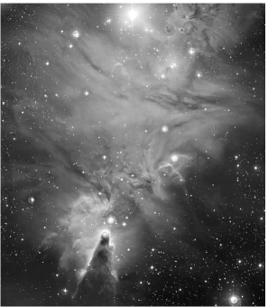
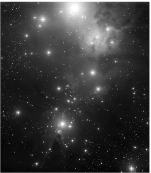
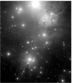
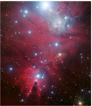
Figure 2: The color image represents a high quality approximation (PSNR 42.5 dB) of an image of the nebula NGC 2264. Credit ESO [30]. The small picture at the top is the RGB folded image. The one right below is the part containing the indices. The three small pictures in the next row are the folded channels (each of which contains coefficients of plain text representation of that channel). The three larger pictures are the channels recovered from the previous ones. The bottom picture is the recovered RGB image. The recovery is successful because it was realized with the authorized key.

In this section the SCEIF approach is illustrated with two examples both involving an RGB color image.

The picture at the bottom of Fig. 2 is an image of the nebula NGC 2264 created at the European Southern Observatory (ESO) [30]. The resolution of this image is $1464\times 1280$ pixels per channel. The $2$D intensity arrays, one for each channel, are the three pictures right above the color one. In order to apply SCEIF firstly each channel is divided into small blocks of $8\times 8$ pixels. The blocks are approximated using the mixed dictionary of Sec.2.2 and the approach of Sec. 2.1. The approximation is of high quality. This is ensured by using two measures on the whole color image: a high PSNR (42.5 dB) and a high Mean Structural Similarity Index (0.997) [32] (further comments are given in Sec. 5.1). Each channel in Fig. 2 is folded and reshaped to produce a single RGB image. The latter is the small picture at the top of Fig. 2. Notice that the size of such an image is ‘extra small’ ($120\times 1280\times 3$ pixels) in comparison to the original ($1464\times 1280\times 3$ pixels). This is because the representation of the full image by the proposed mixed dictionary is very sparse. The SR for the image is 17.42.

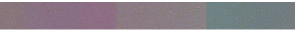
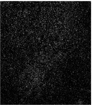
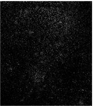
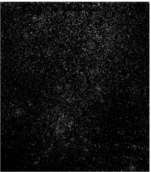
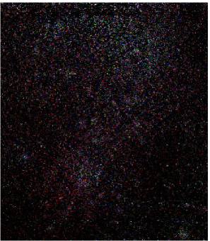
Figure 3: Unsuccessful attempt to expand the image NGC 2264 of Fig. 2 using an incorrect key.

Assuming now that the folded image is given to a partner stored in the original 16-bit RGB format, in order to recover the image the receiver should proceed as follows: first the header information is read. This is not encrypted and is required by the receiver to separate the image components $\tilde{G}$ and $G$, and to reconstruct the three independent folded images, displayed in the third row (from the top) of Fig. 2.

Now the process continues, as prescribed in Sec. 3.2, to recover the channels. The images in the fourth row of Fig. 2 depict the recovered channels using the correct private key, shown together as an RGB image in the last row. Because the authorized key is used, the recovery was successful. Fig. 3 illustrates the identical process using the incorrect private key.

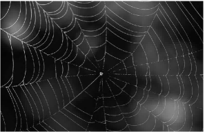
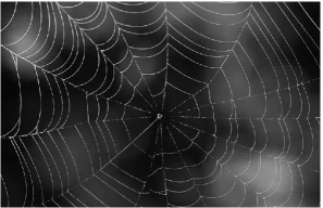
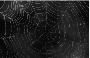
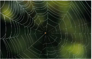
Figure 4: Same description as in Fig. 2 but the image is a close up of a spider web in Australia. Courtesy of National Geographic. Photograph by Darlyne Murawski [31].

Figure 5: Unsuccessful attempt to expand the spider web image of Fig. 4 using an incorrect key.

As a second example we proceed as before, but on a close up of the spider web photo, kindly rendered by National Geographic [31]. There is a difference from the previous case in that, instead of giving free access to the correct number of atoms per block $K_{q},\,q={\tilde{H}}+1,\ldots,Q$, in this example those numbers are also hidden, together with the indices. The reason being that because of the contrast between the blocks containing the web and the rest of the blocks, those numbers give some information about the image. Certainly, by knowing only those numbers one can tell that the image has a very smooth background with some details only where the spider web is located. This gives some visual information that one may want to avoid by hiding those numbers.

The folded image reduces the size of the original spider web photo ($512\times 792\times 3$ pixels) less than in the previous case ($89\times 792\times 3$ pixels) because the SR is smaller: 7.95.

For comparative purposes we have implemented the SCEIF method using DCT, which is also suitable for block processing. The implementation of the folding and encryption steps is exactly the same, the only difference is that the approximation can be performed by DCT, which is straightforward and faster than with the dictionary. However, since the sparsity achieved by DCT is lower (SR= 10.06 for the nebula image and SR = 4.23 for the spider web) the corresponding folded images are larger (see Fig. 6). In addition, because the processing time is dominated by the actual folding and expanding procedures, SCEIF implemented with the mixed dictionary is faster than with DCT (see Table 2).

Figure 6: The first picture in the top line is the folded image (size $120\times 1280\times 3$) of the nebula NGC 2264 (size $1464\times 1280\times 3$) with the proposed dictionary. The second picture in the top line is the folded image (size $202\times 1280\times 3$) with DCT. The pictures in the bottom line, sizes ($89\times 792\times 3$) and ($165\times 792\times 3$), are the folded images with the dictionary and DCT, respectively, of the spider web image (size $512\times 792\times 3$).

		Running times (in secs)
		Approximation	Folding	Expanding	Total
Nebula	Dictionary	10.9	10.7	13.7	35.3
	DCT	Disregarded	17.3	20.3	37.6
Spider web	Dictionary	4.9	4.7	5.6	15.2
	DCT	Disregarded	7.8	8.9	16.7

Table 2: Comparison of the folding and expanding times (average of five independent runs) with the mixed dictionary and DCT. The test was performed with MATLAB using a 14” laptop equipped with 2.8GHz processor and 3GB RAM. As the implementation of the approximation with DCT was not optimized, the approximation times are not included in the calculation of the total execution time with this approach. The approximation with the dictionary was realized using a MEX file in C++ for implementing OMP2DMl to approximate the three channels simultaneously.

5 Quality and security issues

Concerning the quality of the recovered image there are two independent aspects to be discussed. One is the quality of the approximation, $I^{K}$, of the original image $I$ and the other is the quality of the recovery of $I^{K}$.

The security matters that will be discussed are restricted to key sensitivity and resistance to plain text attack.

5.1 Quality

The quality of the approximation, $I^{K}$, of the image $I$ is to be decided beforehand. In the examples we have considered high quality approximations. This is assessed by two standard measures. One is the PSNR, which is defined as

$$\mathrm{PSNR}=10\log_{10}\left(\frac{{(2^{l_{\mathrm{b}}}-1)}^{2}}{\mathrm{MSE}}\right),$$ (16)

where $l_{\mathrm{b}}$ is the number of bits used to represent the intensity of the pixels and

$$\mathrm{MSE}=\frac{\sum_{z=1}^{Z}\|I_{z}-I^{K}_{z}\|_{F}^{2}}{ZN_{x}N_{y}},$$

with $Z=1$ for a gray level image and $Z=3$ for an RGB image.

In the two numerical examples of Sec. 4 the corresponding PSNR is high enough (42.5 dB) to secure approximations of high quality (with no visual degradation with respect to the original image). The other measure we have used to assess the quality of the approximate image is the Mean Structure Similarity index (MSSIM) [32], which for two identical images is equal to one. The MSSIM index between the original image and the approximation, in both examples of Sec. 4, is larger than 0.99. This value complements and confirms the quality indicated by the PSNR.

Once the desired quality of the approximated image has been fixed, that approximation becomes the plain text image to be folded and encrypted. Thus, the next goal is to recover the approximate image with high fidelity. The recovering would be ‘exact’ if not for the quantization step which is introduced to store the folded image using integers. The present version of the proposed scheme works with images stored using 16 bits per channel. At this precision, in both examples, the MSSIM index between the image recovered with the right key and the plain text image is equal to one. The PSNR between the authorized recovered image and the original image is identical to that between the plain text image and the original one.

5.2 Security

The security of the encryption scheme we have adopted relies on the random number generator. The more reliable the random generator is the safer the encryption procedure. Our implementation uses a simple 32-bit pseudo random number generator but, apart from the convenience of having it at hand, there is no reason for using that particular one.

While the key space for the present implementation is $2^{32}$, simply by making access to the order of orthogonalization private (c.f. (10) and (14)) the key space would be expanded.

Key sensitivity: The high sensitivity against small variations in the private key is illustrated by Figures 3 and 5. The failed recovery shown in those figures were attempted using a key differing only by one digit with the correct one. The private key is 1234567891 and the tested key 1234567890. The PSNR between the plain text image and the recovered image with the wrong key is $10.8$dB for the image of Fig. 3 and 9.15 dB for the image of Fig. 5. This sensitivity was verified statistically by repeating the experiment with 100 keys differing in only one digit from the correct key. The mean value of the resultant PSNR for the nebula image is $10.68$dB with standard deviation 1.23. For the spider web image the mean value PSNR is $8.6$dB with standard deviation 1.41.

Prevention of plain text attacks: In order to avoid repetitions of the encryption operators (c.f. (10) and (14)) the random arrays (8) and (12) should be guaranteed to be different every time the procedure is executed. That is the role the public initialization $\mathbf{seed}$ plays at the folding step. The $\mathbf{seed}$ can be set automatically, for instance as the date and time right before the vectors are generated. Thus, the nonlinearity of the operation $\widehat{\mathrm{Orth}}(\cdot)$ prevents an attacker from inverting the system of equations (7) and (15) using correctly decrypted plain text images.

Notice that the public $\mathbf{seed}$ ensures that even the identical plain text image produces a different cipher one. In order to illustrate this feature we calculated the PSNR between two folded images encrypted with the same private key but different public seeds. For the astronomical image the resulting PSNR was 14.25 dB and for spider web 13.78 dB.

6 Conclusions

The recently introduced EIF approach has been extended to SCEIF by introducing the following features:

• The folding capacity of the approach has been improved by considering a new dictionary for the approximation.

• The approach is now self-contained. All that is required to recover the plain text image is the folded (cipher) image and the private key. This is achieved by enlarging the folded image creating ad hoc blocks to place the indexes of those dictionary’s elements participating in the image approximation (plain text image).

• The implementation has also been extended from gray level to color images.

The success of the approach is based on two fundamental and related features: One is the possibility of reducing the data dimensionality by a powerful highly non linear transformation. The other is the possibility of implementing the approach in an affordable period of time. The proposed dictionary plays a central role in ensuring both features, by allowing for processing obeying a scaling law. Certainly, the fact that the approximation of a large image can be realized by dividing it into small blocks is the key of the current effective implementation. It should be emphasized that the numerical examples have been realized on a small laptop in MATLAB environment. Simply by implementing the method in a programming language, such as C or Fortran, the folding and expanding times given in Table 2 could be reduced by up to tenfold. In addition, there is room for straightforward implementation by parallel computing if those resources are available.

Final Remarks

• The scope of SCEIF is to fold an image in encrypted form. The size of the astronomical image is reduced 12.2-fold (pixel wise) and the spider web 5.75-fold. We are not considering here any further compression stage, which could imply to convert the folded image into a bit stream. It should be stressed that, in order to do that, the encoding technique should be especially conceived to deal with the type of data that SCEIF generates by folding the image.

• The simple symmetric key encryption procedure considered here leaves room for straightforward improvement, e.g.,

  a)The key space could be extended by the orthogonalization operation. In the present version the orthogonalization step (c.f. (10) and (14)) is assumed to be completely known. However, simply by making access to the order of orthogonalization private, the key space would be expanded.

  b)The other possibility that can be foreseen, to strengthen the security of the proposed encryption scheme, is to further scramble the folded image using a chaos-based encryption algorithm. Considering the security flaws affecting some of those algorithms [12, 13, 33, 16, 14], it becomes noticeable that our approach could benefit those techniques in a twofold manner: i)providing a way of reducing the image size, and ii)enhancing the security of the algorithms.

For the above reasons the proposed SCEIF approach appears in our mind a very exciting possibility. We feel confident that it will stimulate further work in this direction.

Acknowledgements

Support from EPSRC, UK, grant (EP$/$D062632$/$1) is acknowledged. We are grateful to the European Southern Observatory and National Geographic for authorization to use their images for illustration of the approach. Dedicated open source software for implementation of the approach is available at [28], section SCEIFS.

A. Construction of Matrices $B^{k}_{n},\,n=1,\ldots,k$ (c.f.(5))

For $z=1,2,3$ the coefficients $c_{n}^{z},\,n=1,\ldots,k$ in (4) should be determined in such a way that $\|R_{z}^{k}\|_{\mathrm{F}}$ is minimum for each $z$. This is ensured by requesting that $R_{z}^{k}=I_{z}-\hat{\mathrm{P}}_{\mathbb{V}_{k}}I_{z},\,z=1,2,3$, where $\hat{\mathrm{P}}_{\mathbb{V}_{k}}$ is the orthogonal projection operator onto $\mathbb{V}_{k}={\mbox{\rm{span}}}\{{D}^{x}_{\ell^{x}_{n}}\otimes{D}^{y}_{\ell^{y}_{n}}\}_{n=1}^{k}$. The required representation of $\hat{P}_{\mathbb{V}_{k}}$ is of the form $\hat{P}_{\mathbb{V}_{k}}I=\sum_{n=1}^{k}A_{n}\langle B_{n}^{k},I\rangle_{F}$, where each $A_{n}\in\mathbb{R}^{N_{x}\times N_{y}}$ is an array with the selected atoms $A_{n}={D}^{x}_{\ell^{x}_{n}}\otimes{D}^{y}_{\ell^{y}_{n}}$ and $B_{n}^{k},\,n=1,\ldots,k$ the concomitant reciprocal matrices. These are the unique elements of $\mathbb{R}^{N_{x}\times N_{y}}$ satisfying the conditions:

• $\langle A_{n},B_{m}^{k}\rangle_{\mathrm{F}}=\delta_{n,m}=\begin{cases}1&\mbox{if}\,n=m\\ 0&\mbox{if}\,n\neq m.\end{cases}$

• ${\mathbb{V}_{k}}={\mbox{\rm{span}}}\{B_{n}^{k}\}_{n=1}^{k}.$

Such matrices can be adaptively constructed through the recursion formula [25]:

$$\begin{split}B_{n}^{k+1}&=B_{n}^{k}-B_{k+1}^{k+1}\langle A_{k+1},B_{n}^{k}\rangle_{\mathrm{F}},\quad n=1,\ldots,k,\\ \text{where}\\ B_{k+1}^{k+1}&=W_{k+1}/\|W_{k+1}\|_{\mathrm{F}}^{2},\,\,\text{with}\,\,W_{1}=A_{1}\,\,\text{and}\,\,W_{k+1}=A_{k+1}-\sum_{n=1}^{k}\frac{W_{n}}{\|W_{n}\|_{\mathrm{F}}^{2}}\langle W_{n},A_{k+1}\rangle_{\mathrm{F}}.\end{split}$$ (A.1)

For numerical accuracy in $W_{n},\,n=1,\ldots,k+1$ at least one re-orthogonalization step is usually needed. It implies that one needs to recalculate these matrices as

$$W_{k+1}=W_{k+1}-\sum_{n=1}^{k}\frac{W_{n}}{\|W_{n}\|_{\mathrm{F}}^{2}}\langle W_{n},W_{k+1}\rangle_{\mathrm{F}}.$$ (A.2)

With matrices $B_{n}^{k},\,n=1,\ldots,k$ constructed as above the required coefficients in (3) are obtained, for $z=1,2,3$, from the inner products

$$c^{z}_{n}=\langle B_{n}^{k},I_{z}\rangle_{\mathrm{F}},\,n=1,\ldots,k.$$

References

- [1] A. Uhl, A Pommer, Image and Video Encryption, Springer, NY, (2005).
- [2] B. Furht, D Kirovski (Eds), Multimedia Security Handbook, CRC Press, (2005).
- [3] CH. Yuen, KW. Wong, A chaos-based joint image compression and encryption scheme using DCT and SHA-1, Applied Soft Computing, 11, (2011), 5092–5098.
- [4] OY. Lui, KW Wong, J.Chen, J. Zhou, Chaos-based joint compression and encryption algorithm for generating variable length ciphertext, Applied Soft Computing, 12, (2012), 125–132.
- [5] M. S. Baptista, Cryptography with Chaos, Physics Letters A, 240 (1998) 50–54.
- [6] G. Chen, Y. Mao , C. K. Chui, A symmetric image encryption scheme based on 3D chaotic cat maps, Chaos, Solitons and Fractals 21 (2004) 749–761.
- [7] Y. Mao, G. Chen, S. Lian, A novel fast image encryption schem based on 3D chaotic baker maps, International Jouranl of Bifurcation and Chaos, 14 (2004) 3613–3624.
- [8] S. Lian, J. Sun, Z. Wang, Security analysis of a chaos-based image encryption algorithm, Physica A, 351 (2005) 645–661.
- [9] J.M. Amigó, L. Kocarev, J. Szczepanski, Theory and pratice of chaotic cryptography, Physics Letters A, 366 (2007) 211–216.
- [10] T. Xiang, KW. Wong, X. Liao, Selective image encryption using a spatiotemporal chaotic system, Chaos, 17, 023115 (2007).
- [11] A.N. Pisarchik, M. Zanin, Image encryption with chaotically coupled chaotic maps, Physica D, 237, 20, (2008), 2638–2648.
- [12] D. Arroyo, R. Rhouma, G. Alvarez, S. Li, V. Fernandez, On the security of a new image encryption scheme based on chaotic map lattices, Chaos 18, 033112 (2008).
- [13] D. Arroyo, S. Li, J. M. Amigó, G. Alvarez, R. Rhoumad, Comments on “Image encryption with chaotically coupled chaotic maps”, Physica D, 239 (2010) 1002–1006. DOI: 10.1016/j.physd.2010.02.010.
- [14] E. Solak, C. Çokal, O. T. Yildiz, T. Biyikoglu, Cryptanalysis of Fridrich’s chaotic image encryption, International Journal of Bifurcation and Chaos, 20, (2010) 1405–1413.
- [15] L. Kocarev, S Lian (Eds.), Chaos-based cryptography, studies in cumputational intelligence 354, Springer-Verlag Berlin Heidelberg (2011).
- [16] G. Alvarez, J. M. Amigó, D. Arroyo, S. Li, Lessons learnt from the cryptanalysis of chaos-based ciphers, in [15], 257–295.
- [17] G. Millérioux, J. M. Amigó, J. Daafouz, A connection between chaotic and conventional cryptography, IEEE Transactions on Circuits and Systems, 55, 6 (2008) 1695–1703, DOI:10.1109/TCSI.2008.916555.
- [18] J. Bowley, L. Rebollo-Neira, Sparsity and “Something Else”: An Approach to Encrypted Image Folding, IEEE Siganal Processing Letters 18 (2011) 189–192.
- [19] J. Miotke and L. Rebollo-Neira, Oversampling of Fourier Coefficients for Hiding Messages, Applied and Computational Harmonic Analysis, 16 (2004) 203–207.
- [20] L. Rebollo-Neira, A. Plastino, Statistical distribution, host for encrypted information, Physica A, 359 (2006) 213–221.
- [21] B.D. Rao, K. Engan, S. F. Cotter, J. Palmer, K. Kreutz-Delgado, Subset selection in noise based on diversity measure minimization, IEEE Transactions on Signal Processing, 51, 3 (2003) 760– 770, 10.1109/TSP.2002.808076.
- [22] C. Tsallis, Possible generalization of Boltzmann-Gibbs statistics, J. Stat. Phys., 52 (1988) 479.
- [23] C. Tsallis, Introduction to nonextensive statistical mechanics, Springer-Verlag, NY (2009).
- [24] Y.C. Pati, R. Rezaiifar, and P.S. Krishnaprasad, Orthogonal matching pursuit: recursive function approximation with applications to wavelet decomposition, Proceedings of the 27th Annual Asilomar Conference in Signals, System and Computers, 1 (1993) 40–44.
- [25] L. Rebollo-Neira and D. Lowe, Optimized orthogonal matching pursuit approach, IEEE Signal Processing Letters, 9 (2002) 137–140.
- [26] M. Andrle and L. Rebollo-Neira, A swapping-based refinement of orthogonal matching pursuit strategies, Signal Processing, 86 (2006) 480–495.
- [27] J. A. Tropp, A. C. Gilbert, M. J. Strauss, Algorithms for simultaneous sparse approximation. Part I: Greedy pursuit, Signal Processing, 86 (2006) 572–588.
- [28] http://www.nonlinear-approx.info/
- [29] M. Andrle, L. Rebollo-Neira, Cardinal B-spline dictionaries on a compact interval, Applied and Computational Harmonic Analysis, 18 (2005) 336–346.
- [30] http://www.eso.org/public/images/eso0848a/
-
[31]
http://photography.nationalgeographic.com/photography/enlarge/
australia-spider-web.html - [32] Z. Wang, A. C. Bovik, H. R. Sheikh, E. P. Simoncelli, Image quality assessment: From error visibility to structural similarity, IEEE Transactions on Image Processing, 13 (2004) 600–612.
- [33] A. N. Pisarchik, M. Zanin, Reply to: “Comment on: Image encryption with chaotically coupled chaotic maps”, Physica D, 239, (2010) 1001.