Improved quantum hypergraph-product LDPC codes

Abstract

We suggest several techniques to improve the toric codes and the finite-rate generalized toric codes (quantum hypergraph-product codes) recently introduced by Tillich and Zémor. For the usual toric codes, we introduce the rotated lattices specified by two integer-valued periodicity vectors. These codes include the checkerboard codes, and the family of minimal single-qubit-encoding toric codes with block length $n=t^{2}+(t+1)^{2}$ and distance $d=2t+1$, $t=1,2,\ldots$. We also suggest several related algebraic constructions which increase the rate of the existing hypergraph-product codes by up to four times.

I Introduction

Quantum error correction[1, 2, 3] made quantum computing (QC) theoretically possible. However, high precision required for error correction [4, 5, 6, 7, 8, 9] combined with the large number of auxiliary qubits necessary to implement it, have so far inhibited any practical realization beyond proof-of-the-principle demonstrations[10, 11, 12, 13, 14, 15].

For stabilizer codes, the error syndrome is obtained by measuring the generators of the stabilizer group. The corresponding quantum measurements can be greatly simplified (and also done in parallel) in low-density parity-check (LDPC) codes which are specially designed to have stabilizer generators of small weight. Among LDPC codes, the toric (and related surface) codes [16, 5, 9, 17] have the stabilizer generators of smallest weight, $w=4$, with the support on neighboring sites of a two-dimensional lattice. These codes have other nice properties which make them suitable for quantum computations with relatively high error threshold. Unfortunately, these code families have very low code rates that scale as inverse square of the code distance.

Recently, Tillich and Zémor proposed a finite-rate generalization of toric codes[18]. The construction relates a quantum code to a direct product of hypergraphs corresponding to two classical binary codes. Generally, thus obtained LDPC codes have finite rates and the distances that scale as a square root of the block length. Unfortunately, despite finite asymptotic rates, for smaller block length, the rates of the quantum codes which can be obtained from the construction[18] are small.

In this work, we present a construction aimed to improve the rates of both regular toric[16] and generalized toric codes[18]. For the toric codes, we introduce the rotated tori specified by two integer-valued periodicity vectors. Such codes include the checkerboard codes [17] ($\pi/4$-rotation), and the family [19] of minimal single-qubit-encoding toric codes with block length $n=t^{2}+(t+1)^{2}$ and distance $d=2t+1$, $t=1,2,\ldots$. For the generalized toric codes[18], we suggest an algebraic construction equivalent to the $\pi/4$ rotation of the regular toric codes. The resulting factor of up to four improvement of the code rate makes such codes competitive even at relatively small block sizes.

II Definitions.

We consider binary quantum error correcting codes (QECCs) defined on the complex Hilbert space $\mathcal{H}_{2}^{\otimes n}$ where $\mathcal{H}_{2}$ is the complex Hilbert space of a single qubit $\alpha\left|0\right\rangle+\beta\left|1\right\rangle$ with $\alpha,\beta\in\mathbb{C}$ and $\left|\alpha\right|^{2}+\left|\beta\right|^{2}=1$. Any operator acting on such an $n$-qubit state can be represented as a combination of Pauli operators which form the Pauli group $\mathscr{P}_{n}$ of size $2^{2n+2}$ with the phase multiplier $i^{m}$:

$$\mathscr{P}_{n}=i^{m}\{I,X,Y,Z\}^{\otimes n},\;m=0,\ldots,3\>,$$ (1)

where $X$, $Y$, and $Z$ are the usual Pauli matrices and $I$ is the identity matrix. It is customary to map the Pauli operators, up to a phase, to two binary strings, $\mathbf{v},\mathbf{u}\in\{0,1\}^{\otimes n}$ [20],

$$U\equiv i^{m^{\prime}}X^{\mathbf{v}}Z^{\mathbf{u}}\>\rightarrow(\mathbf{v},\mathbf{u}),$$ (2)

where $X^{\mathbf{v}}=X_{1}^{v_{1}}X_{2}^{v_{2}}\ldots X_{n}^{v_{n}}$ and $Z^{\mathbf{u}}=Z_{1}^{u_{1}}Z_{2}^{u_{2}}\ldots Z_{n}^{u_{n}}$. A product of two quantum operators corresponds to a sum ($\mathop{\rm mod}2$) of the corresponding pairs $(\mathbf{v}_{i},\mathbf{u}_{i})$.

An $[[n,k,d]]$ stabilizer code $\mathcal{Q}$ is a $2^{k}$-dimensional subspace of the Hilbert space $\mathcal{H}_{2}^{\otimes n}$ stabilized by an Abelian stabilizer group $\mathscr{S}=\left\langle G_{1},\ldots,G_{n-k}\right\rangle$, $-{\mathbb{1}}\not\in\mathscr{S}$ [21]. Explicitly,

$$\mathcal{Q}=\{\left|{\psi}\right\rangle:S\left|{\psi}\right\rangle=\left|{\psi}\right\rangle,\forall S\in\mathscr{S}\}.$$ (3)

Each generator $G_{i}\in\mathscr{S}$ is mapped according to Eq. (2) in order to obtain the binary check matrix $H=(A_{X}|A_{Z})$ in which each row corresponds to a generator, with rows of $A_{X}$ formed by $\mathbf{v}$ and rows of $A_{Z}$ formed by $\mathbf{u}$ vectors. For generality, we assume that the matrix $H$ may also contain unimportant linearly dependent rows which are added after the mapping has been done. The commutativity of stabilizer generators corresponds to the following condition on the binary matrices $A_{X}$ and $A_{Z}$:

$$A_{X}A_{Z}^{T}+A_{Z}A_{X}^{T}=0\;(\mathop{\rm mod}2).$$ (4)

A more narrow set of Calderbank-Shor-Steane (CSS) codes [22] contains codes whose stabilizer generators can be chosen to contain products of only Pauli $X$ or Pauli $Z$ operators. For these codes the parity check matrix can be chosen in the form:

$$H=\left(\begin{array}[]{c|c}G_{X}&0\\ 0&G_{Z}\end{array}\right),$$ (5)

where the commutativity condition simplifies to $G_{X}G_{Z}^{T}=0$.

The dimension of a quantum code is $k=n-\mathop{\rm rank}H$; for a CSS code this simplifies to $k=n-\mathop{\rm rank}G_{X}-\mathop{\rm rank}G_{Z}$.

The distance $d$ of the quantum code is given by the minimum weight of an operator $U$ which commutes with all operators from the stabilizer $\mathscr{S}$, but is not a part of the stabilizer, $U\not\in\mathscr{S}$. In terms of the binary vector pairs $(\mathbf{a},\mathbf{b})$, this is equivalent to a minimum weight of the bitwise OR $(\mathbf{a}|\mathbf{b})$ of all pairs satisfying the symplectic orthogonality condition,

$$A_{X}\mathbf{b}+A_{Z}\mathbf{a}=0,$$ (6)

which are not linear combinations of the rows of $H$.

III Toric codes and rotated toric codes

III-A Canonical construction

We consider the toric codes[16] in the restricted sense, with qubits located on the bonds of a square lattice $L_{\xi}\times L_{\eta}$, with periodic boundary conditions along the directions $\xi$ and $\eta$. The stabilizer generators $A_{i}\equiv\prod_{j\in\square_{i}}X_{j}$ and $B_{i}\equiv\prod_{j\in+_{i}}Z_{j}$ are formed as the products of $X_{j}$ around each plaquette, and $Z_{j}$ around each vertex (this defines a CSS code). The corresponding block length is $n=2L_{\xi}L_{\eta}$, and there are $r_{A}=r_{B}=L_{\xi}L_{\eta}-1$ independent generators of each kind, which leaves us with the code of size $k=n-r_{A}-r_{B}=2$. This code is degenerate: the degeneracy group is formed by products of the generators $A_{i}$, $B_{i}$; its elements can be visualized as (topologically trivial) loops drawn on the original lattice (in the case of products of $A_{i}$), or the dual lattice in the case of products of $B_{i}$. The two sets of logical operators are formed as the products of $X$ ($Z$) operators along the topologically non-trivial lines formed by the bonds of the original (dual) lattice (see Fig. 1). The code distance $d=\min(L_{\xi},L_{\eta})$ is given by the minimal weight of such operators.

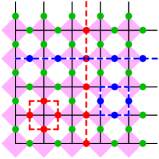
Figure 1: (Color online) Lattice representing the canonical toric code $[[50,2,5]]$. The generators $A_{i}$ are formed by Pauli $X$ generators around a plaquette (blue square) while the generators $B_{i}$ are formed by Pauli $Z$ generators around a vertex (red square). Dashed horizontal blue line and vertical red line represent a pair of mutually conjugate logical operators formed by the products of $X$ and $Z$ respectively. Shading corresponds to an alternative checkerboard representation of the underlying lattice.

III-B Checkerboard codes [17]

In the following, it will be convenient to consider a lattice with qubits placed on the vertices. Then, if we color every other plaquette to form a checkerboard pattern, we can define the operators $A_{i}$ as products of $X$ operators around the colored plaquettes, and the operators $B_{i}$ as products of $Z$ operators around the white plaquettes (see Fig. 2, Left). Now, the checkerboard code with $n=L_{x}L_{y}$, where both $L_{x}$ and $L_{y}$ are even, can be defined by taking periodic boundary conditions on the sides of a rectangle of size $L_{x}\times L_{y}$. The condition ensures that we can maintain a consistent checkerboard pattern. Then, the product of all $A_{i}$ (or of all $B_{i}$) gives identity. Thus, the stabilizer is formed by $n-2$ independent generators, which again gives $k=2$ as in the regular toric codes. The two sets of logical operators are formed by the products of $X$ operators along the topologically non-trivial paths drawn through the colored areas, and the products of $Z$ operators along the topologically non-trivial paths through the white areas (see Fig. 2, Left). The distance of the code, $d=\min(L_{x},L_{y})$, corresponds to the shortest topologically non-trivial chain of qubits, graphically, a horizontal or a vertical straight line.

Figure 2: Left: Lattice representation of the checkerboard code $[[16,2,4]]$. Qubits are placed in the lattice vertices; dashed blue and red lines represent a pair of logical operators as in Fig. 1. Right: same for the rotated checkerboard code $[[10,2,3]]$.

III-C Checkerboard codes with arbitrary rotation

Compared to the regular toric codes, the checkerboard codes use half as many qubits with the same $k$ and distance. The disadvantage is that the distance is always even. This latter restriction can be lifted by introducing periodicity vectors which are not necessarily parallel to the bonds of the lattice. (Note that a similar trick was used in early small-cluster exact diagonalization studies of the Hubbard model[23]).

Let us define two integer-valued periodicity vectors $\mathbf{L}_{i}=(a_{i},b_{i})$, $i=1,2$, and identify all points on the lattice which can be connected by a vector of the form $m_{1}\mathbf{L}_{1}+m_{2}\mathbf{L}_{2}$, with integer $m_{i}$. The checkerboard pattern is preserved iff both $\|\mathbf{L}_{i}\|_{1}\equiv|a_{i}|+|b_{i}|$ are even, $i=1,2$. Such a cluster contains

$$n=|\mathbf{L}_{1}\times\mathbf{L}_{2}|=|a_{1}b_{2}-b_{1}a_{2}|$$ (7)

vertices, and, again, we have $k=2$ as for the standard checkerboard codes.

Since the qubits in the positions shifted by $\mathbf{L}_{i}$ are the same, it is easy to see that our code is identical to that on a cluster with periodicity vectors, e.g., $\mathbf{L}_{1}$, $\mathbf{L}_{1}+\mathbf{L}_{2}$, and, generally, a cluster with periodicity vectors $\mathbf{L}_{i}^{\prime}=g_{ij}\mathbf{L}_{j}$, where the integer-valued matrix $g_{ij}$ has the determinant $\det g=\pm 1$.

For a periodicity vector $\mathbf{L}=(a,b)$ with $a+b$ even, the shortest topologically non-trivial qubit chain has $\|\mathbf{L}\|_{\infty}\equiv\max(|a|,|b|)$ operators which leads to the code distance:

$$d(\mathbf{L}_{1},\mathbf{L}_{2})=\min_{m_{1},m_{2}}\|m_{1}\mathbf{L}_{1}+m_{2}\mathbf{L}_{2}\|_{\infty}.$$ (8)

Example 1.

A family of near-optimal odd-distance checkerboard codes can be introduced by taking $\mathbf{L}_{1}=(2t+1,1)$, $\mathbf{L}_{2}=(-1,2t+1)$, $t=1,2,\ldots$. Such codes have the parameters $[[1+(2t+1)^{2},2,2t+1]]$; explicitly: $[[10,2,3]]$ (illustrated in Fig. 2, Right), $[[26,2,5]]$, $[[50,2,7]]$, ….

Example 2.

The original toric codes are recovered by taking $\mathbf{L}_{i}$ along the diagonals, $\mathbf{L}_{1}=(L_{\xi},L_{\xi})$, $\mathbf{L}_{2}=(-L_{\eta},L_{\eta})$, so that $\|L_{i}\|_{1}$ are always even, thus $n=2L_{\xi}L_{\eta}$, $k=2$, and $d=\min(L_{\xi},L_{\eta})$. For odd distances, taking $L_{\xi}=L_{\eta}=d$, we have the codes $[[18,2,3]]$, $[[50,2,5]]$, $[[98,2,7]]$, ….

III-D Non-bipartite rotated toric codes

We now construct a version of rotated toric codes on clusters with at least one of the periodicity vectors $\mathbf{L}_{i}$ violating the checkerboard pattern, e.g., $\|\mathbf{L}_{1}\|_{1}$ odd. Since the checkerboard pattern cannot be maintained, we define identical stabilizer generators in a non-CSS form, with the stabilizer generators $G_{i}=ZXXZ$ on each plaquette given by the products of $Z$ operators along one diagonal, and $X$ operators along the other diagonal. With periodic boundary conditions, the product of all $G_{i}$ is an identity, and this is the only relation between these operators on a non-bipartite cluster. Thus, here we have only one encoded qubit, $k=1$.

The operators $G_{i}$ can be viewed as local Clifford (LC) transformed $A_{i}$ or $B_{i}$ operators of the toric code. It is easy to see that the logical operators have to correspond to topologically non-trivial closed chains of qubits, as for the bipartite case. However, in order to close the loop, we have to take only the translation vectors with $\|\mathbf{L}\|_{1}$ even. For example, if $\|\mathbf{L}_{1}\|_{1}$ is odd and particularly small, the minimal chain could wrap twice around the direction given by $\mathbf{L}_{1}$. Since the two turns could share some of the qubits, it is difficult to come up with a general expression for the distance.

Example 3.

Checkerboard-like codes can be obtained by taking $L_{x}$ or $L_{y}$ odd. Smallest codes in this family correspond to $L_{x}=L_{y}=d$; they have parameters $[[d^{2},1,d]]$, where $d=2t+1$. Explicitly, $[[9,1,3]]$, $[[25,1,5]]$, $[[49,1,7]]$, ….

Example 4.

A family of smallest odd-distance rotated toric codes [19] is obtained for $\mathbf{L}_{1}=(t+1,t)$, $\mathbf{L}_{2}=(-t,t+1)$, $t=1,2,\ldots$. These codes have the parameters $[[t^{2}+(t+1)^{2},1,2t+1]]$. Explicitly, $[[5,1,3]]$, $[[13,1,5]]$, $[[25,1,7]]$, $[[41,1,9]]$, ….

IV Generalized toric and checkerboard codes

IV-A Algebraic representation of hypergraph-product codes

The finite-rate generalization[18] of the toric code relies on hypergraph theory, with the square lattice generalized to a product of hypergraphs (each corresponding to a parity check matrix of a classical binary code). We first recast the original construction into an algebraic language.

Let $\mathcal{H}_{1}$ (dimensions $r_{1}\times n_{1}$) and $\mathcal{H}_{2}$ (dimensions $r_{2}\times n_{2}$) be two binary matrices. The associated (hypergraph-product) quantum code[18] is a CSS code with the stabilizer generators

$$\begin{array}[]{c}\displaystyle G_{X}=(E_{2}\otimes\mathcal{H}_{1},\mathcal{H}_{2}\otimes E_{1}),\\ \displaystyle G_{Z}=(\mathcal{H}_{2}^{T}\otimes\widetilde{E}_{1},\widetilde{E}_{2}\otimes\mathcal{H}_{1}^{T}).\end{array}$$ (9)

Here each matrix is composed of two blocks constructed as Kronecker products (denoted with “$\otimes$”), and $E_{i}$ and $\widetilde{E}_{i}$, $i=1,2$, are unit matrices of dimensions given by $r_{i}$ and $n_{i}$, respectively. The matrices $G_{X}$ and $G_{Z}$, respectively, have $r_{1}r_{2}$ and $n_{1}n_{2}$ rows (not all of the rows are linearly independent), and they both have $n\equiv r_{2}n_{1}+r_{1}n_{2}$ columns, which gives the block length of the quantum code. The commutativity condition $G_{X}G_{Z}^{T}=0$ is obviously satisfied by Eq. (9) since the Kronecker product obeys $(A\otimes B)(C\otimes D)=AC\otimes BD$.

Note that the construction (9) is somewhat similar to product codes introduced by Grassl and Rötteler[24]. The main difference is that here the check matrix and not the generator matrix is written in terms of direct products.

The parameters $[[n,k,d]]$ of thus constructed quantum code are determined by those of the four classical codes which use the matrices $\mathcal{H}_{1}$, $\mathcal{H}_{2}$, $\mathcal{H}_{1}^{T}$, and $\mathcal{H}_{2}^{T}$ as the parity-check matrices. The corresponding parameters are introduced as

$$\mathcal{C}_{\mathcal{H}_{i}}=[n_{i},k_{i},d_{i}],\quad\mathcal{C}_{\mathcal{H}_{i}^{T}}=[{\widetilde{n}}_{i},\widetilde{k}_{i},\widetilde{d}_{i}],\quad i=1,2,$$ (10)

where we use the convention [18] that the distance $d_{i}(\widetilde{d}_{i})=\infty$ if $k_{i}(\widetilde{k}_{i})=0$. The matrices $\mathcal{H}_{i}$ are arbitrary, and are allowed to have linearly-dependent rows and/or columns. As a result, both $k_{i}=n_{i}-\mathop{\rm rank}\mathcal{H}_{i}$ and $\widetilde{k}_{i}=\widetilde{n}_{i}-\mathop{\rm rank}\mathcal{H}_{i}$ can be non-zero at the same time as the block length of the “transposed” code $\mathcal{C}_{\mathcal{H}_{i}^{T}}$ is given by the number of rows of $\mathcal{H}_{i}$, $\widetilde{n}_{i}=r_{i}$.

Specifically, for the hypergraph-product code (9), we have $n=r_{2}n_{1}+r_{1}n_{2}$, $k=2k_{1}k_{2}-k_{1}s_{2}-k_{2}s_{1}$ with $s_{i}=n_{i}-r_{i},\,i=1,2\,$ (Theorem 7 from Ref. [18]), while the distance $d$ satisfies the conditions $d\geq\min(d_{1},d_{2},\widetilde{d}_{1},\widetilde{d}_{2})$ (Theorem 9 from Ref. [18]), and two upper bounds (Lemma 10 from Ref. [18]): if $k_{1}>0$ and $\widetilde{k}_{2}>0$, then $d\leq d_{1}$; if $k_{2}>0$ and $\widetilde{k}_{1}>0$, then $d\leq d_{2}$.

These parameters can also be readily established from the stabilizer generators in the form of Eq. (9). For example, the dimension of the quantum code follows from

Proposition 1.

The number of linearly independent rows in matrices $G_{X}$ and $G_{Z}$ given by Eq.  (9) is $\mathop{\rm rank}G_{X}=r_{1}r_{2}-\widetilde{k}_{1}\widetilde{k}_{2}$ and $\mathop{\rm rank}G_{Z}=n_{1}n_{2}-k_{1}k_{2}$.

Proof.

The matrices $G_{X}$ and $G_{Z}$ have $r_{1}r_{2}$ and $n_{1}n_{2}$ rows, respectively. To count the number of linearly-dependent rows in $G_{X}$, we notice that the equations $(a^{T}\otimes b^{T})\cdot(E_{2}\otimes\mathcal{H}_{1})=0$ and $(a^{T}\otimes b^{T})\cdot(\mathcal{H}_{2}\otimes E_{1})=0$ are both satisfied iff $a\in\mathcal{C}_{\mathcal{H}_{2}^{T}}$ and $b\in\mathcal{C}_{\mathcal{H}_{1}^{T}}$, thus there are $\widetilde{k}_{1}\widetilde{k}_{2}$ linear relations between the rows of $G_{X}$, and we are left with $r_{1}r_{2}-\widetilde{k}_{1}\widetilde{k}_{2}$ linearly-independent rows. Similarly, there are $n_{1}n_{2}-k_{1}k_{2}$ linearly independent rows in $G_{Z}$. ∎

To prove the lower bound on the distance, consider a vector $\mathbf{u}$ such that $G_{X}\cdot\mathbf{u}=0$ and $\mathop{\rm wgt}(\mathbf{u})<d$. We construct a quantum code in the form (9) from the matrices $\mathcal{H}_{1}^{\prime}$, $\mathcal{H}_{2}^{\prime}$ formed only by the columns of respective $\mathcal{H}_{i}$, $i=1,2$, that are involved in the product $G_{X}\cdot\mathbf{u}$. According to Proposition 1, the reduced code has $k=0$, so that the reduced $\mathbf{u}^{\prime}$, $G_{X}^{\prime}\cdot\mathbf{u}^{\prime}=0$, has to be a linear combination of the rows of $G_{Z}^{\prime}$. The rows of $G_{Z}^{\prime}$ are a subset of those of $G_{Z}$, with some all-zero columns removed; thus the full vector $\mathbf{u}$ is also a linear combination of the rows of $G_{Z}$. Similarly, a vector $\mathbf{v}$ such that $G_{Z}\cdot\mathbf{v}=0$ and $\mathop{\rm wgt}(\mathbf{v})<d$, is a linear combination of rows of $G_{X}$.

The upper bound is established by considering vectors $\mathbf{u}\equiv(\mathbf{e}\otimes\mathbf{c},0)$ with $\mathbf{c}\in\mathcal{C}_{\mathcal{H}_{1}}$, which requires $k_{1}>0$. Vector $\mathbf{e}$, $\mathop{\rm wgt}(\mathbf{e})=1$, for which $\mathbf{u}$ is not a linear combination or rows of $G_{Z}$, exists only when $\widetilde{k}_{2}>0$. The other upper bound is established by considering vectors $(0,\mathbf{c}\otimes\mathbf{e})$ with $\mathbf{c}\in\mathcal{C}_{\mathcal{H}_{2}}$.

IV-B Original code family from full-rank matrices

In Ref. [18], only one large family of quantum codes based on the hypergraph-product ansatz (9) is given. Namely, the matrix $\mathcal{H}_{1}$ is taken as a full-rank parity matrix of a binary LDPC code with parameters $\mathcal{C}_{\mathcal{H}_{1}}=[n_{1},k_{1},d_{1}]$ ($r_{1}=n_{1}-k_{1}$), so that the transposed code has dimension zero, $\widetilde{k}_{1}=0$. The second matrix is taken as $\mathcal{H}_{2}=\mathcal{H}_{1}^{T}$, so that $\mathcal{C}_{\mathcal{H}_{2}^{T}}=\mathcal{C}_{\mathcal{H}_{1}}$. Then Eq. (9) defines a quantum LDPC code with parameters

$$\mathcal{Q}^{\mathrm{orig}}=[[(n_{1}-k_{1})^{2}+n_{1}^{2},k_{1}^{2},d_{1}]],$$ (11)

where the weight of each row of $G_{X}$, $G_{Z}$ equals to the sum of the row-weight and the column-weight of $\mathcal{H}_{1}$.

Example 5.

Let $\mathcal{H}_{1}$ be a parity-check matrix of the repetition code $[d,1,d]$. Then the quantum code has the parameters $[2d^{2}-2d+1,1,d]$. Explicitly, $[[13,1,3]]$, $[[25,1,4]]$, $[[41,1,5]]$,…— these parameters are inferior compared to the original toric code family, cf. Examples 3, 4.

IV-C Code family from square matrices

Instead of using full-rank parity-check matrices[18], let us start with a pair of binary codes with square parity-check matrices $\mathcal{H}_{i}$, such that $\widetilde{d}_{1}=d_{1}$, $\widetilde{d}_{2}=d_{2}$. Then, automatically, $\widetilde{k}_{i}=k_{i}=n_{i}-\mathop{\rm rank}\mathcal{H}_{i}$. The hypergraph-product ansatz (9) gives the code with the parameters

$$\mathcal{Q}^{\rm square}=[[2n_{1}n_{2},2k_{1}k_{2},\min(d_{1},d_{2})]].$$ (12)

Note that the rate $R=k/n$ of this family is up to twice that of the family originally suggested in Ref. [18], see Sec. IV-B.

Example 6.

The standard toric codes are recovered by taking for $\mathcal{H}_{2}=\mathcal{H}_{1}$ the circulant matrix of a repetition code. The code parameters are $[[2d_{1}^{2},2,d_{1}]]$, cf. Example 2.

We suggest two general ways to obtain suitable square parity check matrices. First, if we start from an $[n_{1},k_{1},d_{1}]$ LDPC code with the full-rank parity check matrix $P$, we can construct the following symmetric matrix,

$$\mathcal{H}_{1}^{\rm sym}=\left(\begin{array}[c]{cc}\mathbb{1}&P\\ P^{T}&0\end{array}\right),$$ (13)

so that the code $\mathcal{C}_{\mathcal{H}_{1}^{\rm sym}}$ is a $[2n_{1}-k_{1},k_{1},d_{1}]$ LDPC code.

Second construction assumes that $\mathcal{C}_{\mathcal{H}_{i}}$ are cyclic LDPC codes. The full circulant matrices $\mathcal{H}_{i}$ are constructed from coefficients of check polynomials $h_{i}(x)$. The check polynomials of the transposed code, $\widetilde{h}_{i}(x)=h_{i}(x^{n_{i}-1})\mathop{\rm mod}(x^{n_{i}}-1)$, are just the original check polynomials reversed, and the original and transposed codes have the same parameters.

IV-D Code family from symmetric matrices.

If we have two symmetric parity-check matrices, $\mathcal{H}_{i}=\mathcal{H}_{i}^{T}$, $i=1,2$ [e.g., from Eq. (13)], the full hypergraph-product code (9) can be transformed into a direct sum of two independent codes, each with the following non-CSS check matrix

$$H=(E_{2}\otimes\mathcal{H}_{1}|\mathcal{H}_{2}\otimes E_{1}),\quad\mathcal{H}_{i}^{T}=\mathcal{H}_{i},\quad i=1,2.$$ (14)

This gives the following

Theorem 1.

A quantum code in Eq. (14) has parameters

$$\mathcal{Q}^{\rm sym}=[[n_{1}n_{2},k_{1}k_{2},\min(d_{1},d_{2})]].$$ (15)

Thus, we can reduce by half both the blocklength and the number of encoded qubits, i.e., keeping the rate of Eq. (12) but doubling the relative distance.

For a cyclic LDPC code $\mathcal{C}_{\mathcal{H}}$ with a palindromic check polynomial, $x^{\deg h(x)}h(1/x)=h(x)$, such that $n-\deg h(x)$ is even, we can always construct a symmetric circulant matrix $\mathcal{H}$ from the polynomial $x^{[n-\deg h(x)]/2}h(x)$.

Example 7.

If $\mathcal{H}_{1}=\mathcal{H}_{2}$ are symmetric check matrices of a cyclic $[n_{1},k_{1},d_{1}]$ code corresponding to a palindromic polynomial $h(x)$, then the quantum code has parameters $[[n_{1}^{2},k_{1}^{2},d_{1}]]$. In particular, for $n_{1}=17$ and $h(x)=1+x^{3}+x^{4}+x^{5}+x^{6}+x^{9}$ we obtain $[[289,81,5,w=12]]$ code, and for $h(x)=1+x$, we recover the non-bipartite checkerboard codes from Example 3.

IV-E Code family from two-tile codes

Finally, let us construct a generalization of the regular “bipartite” checkerboard codes. We start with a pair of binary codes with the parity check matrices of even size

$$\mathcal{H}_{1}=\tbinom{10}{01}\otimes a_{1}+\tbinom{01}{10}\otimes b_{1},\quad\mathcal{H}_{2}^{p}=a_{2}\otimes\tbinom{10}{01}+b_{2}\otimes\tbinom{01}{10},$$ (16)

constructed from the half-size matrices (“tiles”) $a_{i}$, $b_{i}$ with the distances of the classical codes $\mathcal{C}_{\mathcal{H}_{i}}$ and $\mathcal{C}_{\mathcal{H}_{i}^{T}}$ given by $d_{i}$ and $\widetilde{d}_{i}$, $i=1,2$, where the check matrix $\mathcal{H}_{2}=\tbinom{10}{01}\otimes a_{2}+\tbinom{01}{10}\otimes b_{2}$ is equivalent to $\mathcal{H}_{2}^{p}$ and can be rendered to the latter form by row and column permutations. It is convenient to introduce notation for the dimensionality of symmetric subspaces of $\mathcal{C}_{\mathcal{H}_{1}}$ and $\mathcal{C}_{\mathcal{H}_{2}^{p}}$ containing only words of type ${1\choose 1}\otimes\alpha_{1}$ and $\alpha_{2}\otimes{1\choose 1}$ as $k_{i}^{s}\equiv n_{i}/2-\mathop{\rm rank}(a_{i}+b_{i})$, and for asymmetric subspaces as $k_{i}^{a}\equiv k_{i}-k_{i}^{s}$, $i=1,2$ (analogously we define $\widetilde{k}_{i}^{s}$ and $\widetilde{k}_{i}^{a}$). We define half-size CSS matrices [cf. Eq. (9)]

$$\begin{array}[]{c}G_{X}=(E_{2}^{({1/2})}\otimes\mathcal{H}_{1},\mathcal{H}_{2}^{p}\otimes E_{1}^{({1/2})}),\\ G_{Z}=(\mathcal{H}_{2}^{pT}\otimes\widetilde{E}_{1}^{({1/2})},\widetilde{E}_{2}^{({1/2})}\otimes\mathcal{H}_{1}^{T}),\end{array}$$ (17)

where the identity matrices $E_{i}^{(1/2)}$, $\widetilde{E}_{i}^{(1/2)}$ have dimensions $r_{i}/2$, $n_{i}/2$, half-size compared to those in Eq. (9).

Proposition 2.

The numbers of linearly independent rows in matrices (17) are $\mathop{\rm rank}G_{X}=r_{1}r_{2}/2-\widetilde{k}_{1}^{s}\widetilde{k}_{2}^{s}-\widetilde{k}_{1}^{a}\widetilde{k}_{2}^{a}$ and $\mathop{\rm rank}G_{Z}=n_{1}n_{2}/2-k_{1}^{s}k_{2}^{s}-k_{1}^{a}k_{2}^{a}$.

Proof.

To count the number of linearly-dependent rows in $G_{X}$, we notice that the equations $\upsilon^{T}\cdot(E_{2}^{({1/2})}\otimes\mathcal{H}_{1})=0$ and $\upsilon^{T}\cdot(\mathcal{H}_{2}\otimes E_{1}^{({1/2})})=0$ are both satisfied for ansatz

$$\upsilon=\alpha_{1}\otimes{\alpha_{3}\choose\alpha_{4}}+\alpha_{2}\otimes{\alpha_{4}\choose\alpha_{3}},$$ (18)

if and only if either (i) $\alpha_{1}\neq\alpha_{2}$, $\alpha_{3}\neq\alpha_{4}$ and ${\alpha_{1}\choose\alpha_{2}}\in\mathcal{C}_{\mathcal{H}_{2}^{T}}$, ${\alpha_{3}\choose\alpha_{4}}\in\mathcal{C}_{\mathcal{H}_{1}^{T}}$ or (ii) $\upsilon=\alpha_{1}^{\prime}\otimes{1\choose 1}\otimes\alpha_{3}^{\prime}$ and $\alpha_{1}^{\prime}\in\mathcal{C}_{a_{2}^{T}+b_{2}^{T}}$, $\alpha_{3}^{\prime}\in\mathcal{C}_{a_{1}^{T}+b_{1}^{T}}$, thus there are $\widetilde{k}_{1}^{s}\widetilde{k}_{2}^{s}+\widetilde{k}_{1}^{a}\widetilde{k}_{2}^{a}$ linear relations between the rows in $G_{X}$, and we are left with $\mathop{\rm rank}G_{X}=r_{1}r_{2}/2-\widetilde{k}_{1}^{s}\widetilde{k}_{2}^{s}-\widetilde{k}_{1}^{a}\widetilde{k}_{2}^{a}$ linearly-independent rows. Similarly, we prove that $\mathop{\rm rank}G_{Z}=n_{1}n_{2}/2-k_{1}^{s}k_{2}^{s}-k_{1}^{a}k_{2}^{a}$. ∎

Theorem 2.

A quantum CSS code in Eqs. (16) and (17) has the parameters:

$$\begin{array}[]{c}n=(n_{1}r_{2}+n_{2}r_{1})/2,\\ k=2k_{1}^{s}k_{2}^{s}+2k_{1}^{a}k_{2}^{a}-k_{1}s_{2}/2-k_{2}s_{1}/2,\\ d\geq\min(d_{1}/2,d_{2}/2,\widetilde{d}_{1}/2,\widetilde{d}_{2}/2),\end{array}$$ (19)

where $s_{i}=n_{i}-r_{i}$, $i=1,2$. In addition, for $k_{1}>0$ and $\widetilde{k}_{2}>0$ the upper bound $d\leq d_{1}$ exists and for $k_{2}>0$ and $\widetilde{k}_{1}>0$ the upper bound $d\leq d_{2}$ exists.

Proof.

The number of encoded qubits $k$ follows from Proposition 2. The lower bound on the distance can be established as for the original hypergraph-product codes in Sec. IV-A, except now the reduced binary check matrices $\mathcal{H}_{1}^{\prime}$, $\mathcal{H}_{2}^{\prime}$ should preserve the tiled form (16). Hence, for every column involved in the product $G_{X}\cdot\mathbf{u}$, we may need to insert two columns into the reduced matrices; thus we need $\mathop{\rm wgt}(\mathbf{u})<d/2$ which reduces the lower bound on the distance. The two upper bounds can be established by considering vectors $(\mathbf{e}\otimes\mathbf{c},0)$ with $\mathbf{c}\in\mathcal{H}_{1}$ and $(0,\mathbf{c}\otimes\mathbf{e})$ with $\mathbf{c}\in\mathcal{H}_{2}$, exactly as for the hypergraph-product codes in Sec. IV-A. ∎

Theorem 3.

Suppose $a_{i}$ and $b_{i}$, $i=1,2$ in Eq. (16) are such that $k_{i}^{a}=0$, $k_{i}^{s}\neq 0$, $r_{i}=n_{i}$ and binary codes with generator matrices $a_{i}+b_{i}$ and $a_{i}^{T}+b_{i}^{T}$ are not distance $1$ codes. Then the quantum code in Eq. (17) has parameters $[[n_{1}n_{2},2k_{1}k_{2},\min(d_{1},d_{2},\widetilde{d}_{1},\widetilde{d}_{2})]]$, cf. Eq. (12).

The proof is similar to the proof of Theorem 2. The additional restrictions on the binary codes guarantee that a vector $\mathbf{u}$ of weight less than $d$ can only overlap with columns of $\mathcal{H}_{i}$ in less than $d$ positions even after the symmetric counterparts are added.

If we start from distance-$d$ LDPC codes with half size square parity matrices $\mathcal{H}_{i}^{(1/2)}$ [e.g., from Eq. (13)] then $a_{i}=\mathcal{H}_{i}^{(1/2)}+E^{(1/2)}$ and $b_{i}=E^{(1/2)}$ in Eq. (16) lead to distance-$2d$ code satisfying Theorem 3. Alternatively, one can start with two cyclic LDPC codes with even blocksize $n_{i}$, $i=1,2$, and the check polynomials $h_{i}(x)$ that divide $x^{n_{i}/2}-1$. The corresponding square circulant parity-check matrices $\mathcal{H}_{1}$ and $\mathcal{H}_{2}$ (and $\mathcal{H}_{2}^{p}$) satisfy (16). The generator polynomials,

$$g_{i}(x)=(x^{n_{i}}-1)/h_{i}(x)=(x^{n_{i}/2}+1)\,(x^{n_{i}/2}-1)/h_{i}(x),$$ (20)

and their reversed indicate that $k_{i}^{a}=0$.

Example 8.

If $\mathcal{H}_{1}$ is the square parity matrix of a cyclic $[n_{1},k_{1},d_{1}]$ code corresponding to the polynomial $h(x)$ that divides $1-x^{n_{1}/2}$ and $\mathcal{H}_{2}=\mathcal{H}_{1}$ then the quantum code has parameters $[[n_{1}^{2},2k_{1}^{2},d_{1}]]$. For $n_{1}=30$ and $h(x)=1+x+x^{3}+x^{5}$ we obtain $[[900,50,14,w=8]]$ code. For $h(x)=1+x$, we recover the bipartite checkerboard codes from Sec. III-B.

V Conclusions

We suggested several simple techniques to improve existing quantum LDPC codes, toric codes, and generalized toric codes with asymptotically finite rate (quantum hypergraph-product codes[18]). In the latter case we increased the rate of the code family originally proposed in Ref. [18] by up to four times.

References

• [1] P. W. Shor, Phys. Rev. A, vol. 52, p. R2493, 1995.
• [2] E. Knill and R. Laflamme, Phys. Rev. A, vol. 55, pp. 900–911, 1997.
• [3] C. Bennett, D. DiVincenzo, J. Smolin, and W. Wootters, Phys. Rev. A, vol. 54, p. 3824, 1996.
• [4] E. Knill, R. Laflamme, and W. H. Zurek, Science, vol. 279, p. 342, 1998.
• [5] E. Dennis, A. Kitaev, A. Landahl, and J. Preskill, J. Math. Phys., vol. 43, p. 4452, 2002.
• [6] A. M. Steane, Phys. Rev. A, vol. 68, p. 042322, 2003.
• [7] A. G. Fowler, C. D. Hill, and L. C. L. Hollenberg, Phys. Rev. A, vol. 69, p. 042314, 2004.
• [8] A. G. Fowler, S. J. Devitt, and L. C. L. Hollenberg, Quant. Info. Comput., vol. 4, p. 237, 2004, quant-ph/0402196.
• [9] R. Raussendorf and J. Harrington, Phys. Rev. Lett., vol. 98, p. 190504, 2007.
• [10] L. M. K. Vandersypen, M. Steffen, G. Breyta, C. S. Yannoni, R. Cleve, and I. L. Chuang, Phys. Rev. Lett., vol. 85, pp. 5452–5455, 2000.
• [11] L. M. K. Vandersypen, M. Steffen, G. Breyta, C. S. Yannoni, M. H. Sherwood, and I. L. Chuang, Nature, vol. 414, pp. 883–887, 2001.
• [12] S. Gulde, M. Riebe, G. P. T. Lancaster, C. Becher, J. Eschner, H. Häffner, F. Schmidt-Kaler, I. L. Chuang, and R. Blatt, Nature, vol. 421, pp. 48–50, 2003.
• [13] J. Chiaverini, D. Leibfried, T. Schaetz, M. D. Barrett, R. B. Blakestad, J. Britton, W. M. Itano, J. D. Jost, E. Knill, C. Langer, R. Ozeri, and D. J. Wineland, Nature, vol. 432, p. 602, 2004.
• [14] A. Friedenauer, H. Schmitz, J. T. Glueckert, D. Porras, and T. Schaetz, Nature Physics, 2008.
• [15] K. Kim, M.-S. Chang, S. Korenblit, R. Islam, E. E. Edwards, J. K. Freericks, G.-D. Lin, L.-M. Duan, and C. Monroe, Nature, vol. 465, pp. 590–593, 2010.
• [16] A. Y. Kitaev, Ann. Phys., vol. 303, p. 2, 2003.
• [17] H. Bombin and M. A. Martin-Delgado, Phys. Rev. A, vol. 76, no. 1, p. 012305, Jul 2007.
• [18] J.-P. Tillich and G. Zémor, in Information Theory, 2009. ISIT 2009. IEEE International Symposium on, 28 2009-july 3 2009, pp. 799 –803.
• [19] A. A. Kovalev, I. Dumer, and L. P. Pryadko, Phys. Rev. A, vol. 84, p. 062319, Dec 2011.
• [20] A. R. Calderbank, E. M. Rains, P. M. Shor, and N. J. A. Sloane, IEEE Trans. Inf. Th., vol. 44, pp. 1369–1387, 1998.
• [21] D. Gottesman, Ph.D. thesis, 1997, arXiv:quant-ph/9705052.
• [22] A. R. Calderbank and P. W. Shor, Phys. Rev. A, vol. 54, no. 2, pp. 1098–1105, Aug 1996.
• [23] E. Dagotto, R. Joynt, A. Moreo, S. Bacci, and E. Gagliano, Phys. Rev. B, vol. 41, pp. 9049–9073, May 1990.
• [24] M. Grassl and M. Rotteler, in Information Theory, 2005. ISIT 2005. Proceedings. International Symposium on, sept. 2005, pp. 1018 –1022.