Non-equilibrium spatial distribution of Rashba spin torque in ferromagnetic metal layer

Abstract

We study the spatial distribution of spin torque induced by a strong Rashba spin-orbit coupling (RSOC) in a ferromagnetic (FM) metal layer, using the Keldysh non-equilibrium Green’s function method. In the presence of the $s$-$d$ interaction between the non-equilibrium conduction electrons and the local magnetic moments, the RSOC effect induces a torque on the moments, which we term the Rashba spin torque.

A correlation between the Rashba spin torque and the spatial spin current is presented in this work, clearly mapping the spatial distribution of Rashba spin torque in a nano-sized ferromagnetic device. When local magnetism is turned on, the out-of-plane ($S_{z}$) Spin Hall effect (SHE) is disrupted, but rather unexpectedly an in-plane ($S_{y}$) SHE is detected. We also study the effect of Rashba strength ($\alpha_{R}$) and splitting exchange ($\Delta$) on the non-equilibrium Rashba spin torque averaged over the device. Rashba spin torque allows an efficient transfer of spin momentum such that a typical switching field of 20 mT can be attained with a low current density of less than $10^{7}$A/$\mathrm{cm}^{2}$.

I Introduction

Ever since the theoretical prediction of the spin transfer torque (STT) slonczewski:jmmm159 ; berger:9353 , there has been much research effort in utilizing the STT phenomenon to induce magnetization switching and precession in ferromagnetic (FM) nanostructures without the need for an externally applied magnetic field. Devices which rely on the STT effect for magnetization switching offer the advantages of lower power consumption and reduced device dimension, which are crucial factors for nanoscale and high-density spintronic applications. The STT effect has been studied in conventional magnetic nanostructures such as spin valves katine:prl3149 and magnetic tunneling junctions huai:apl84 . For STT to occur in these magnetic multilayers, one requires a pair of FM layers, i.e., a reference spin layer to generate a spin-polarized current for injection into the second free (switchable) layer. The two layers are magnetized in a noncollinear configuration so as to induce the transfer of the transverse spin momentum from the reference to the free layer, which is mediated by conduction electrons flowing between the two layers. In the above process, the role of the spin-orbit coupling (SOC) effect is neglected. However, it is well-established that SOC can generate a nonequilibrium spin accumulation under the passage of current. Thus, it is conceivable that, in the presence of strong SOC effect, one can induce a STT without the need for an additional reference FM layer. This is corroborated by previous theoretical work which showed that the presence of Rashba spin-orbit coupling (RSOC) whose strength is denoted by $\alpha_{R}$, and exchange interaction $\Delta$ between conduction electrons and local spins, can give rise to domain wall motion via spin momentum transfer obata:prb77 . The same spin transfer mechanism can also occur in a FM layer with a large $\alpha_{R}$ and $\Delta$ values tan:annal326 ; manchon:prb78 . The predicted RSOC-induced spin momentum transfer was experimentally demonstrated in a nanowire array mihai:natm9 ; pi:apl97 . The above findings suggest that by utilizing Rashba-induced STT, one can achieve magnetization switching within a single FM layer, without an additional non-collinear FM layer. Such single layer switching holds several potential advantages over conventional STT devices, such as a more symmetric current switching profile and the reduced influence of spin depolarization at the interfaces.

A key element which determines the feasibility of Rashba STT is the presence of a strong Rashba SOC in the FM metal layer. Initial studies on the Rashba effect were focused on semiconductor (SC) materials miller:prl90 ; sato:jap89 ; giglberger:prb75 ; larionov:prb78 ; akabori:prb77 , especially in two-dimensional electron gas (2DEG) heterojunction structures, which consist of two SC layers with different energy bandgaps. The conduction electrons in the 2DEG experience a strong RSOC effect due to the large potential gradient, as a result of the band-bending at the heterojunction interface. However, utilizing the Rashba-induced STT in SC materials is not an attractive proposition as SCs are intrinsically non-magnetic. Even if ferromagnetic behavior can be induced in them via doping (e.g. in dilute magnetic semiconductors or DMS), the resulting Curie temperature lies well below room temperature. Recent studies have shown, however, that a strong RSOC effect can also be induced in metallic nanostructures, both of the FM and non-FM types lashell:prl77 ; ast:prl98 ; cercellier:prb73 ; krupin:prb71 . It is known that the Rashba SOC requires a structural inversion asymmetry (SIA), which gives rise to an internal electric field. In a metallic FM layer, the SIA can be enhanced by adjacent layers of heavy metals and oxides, which create the requisite band structure mismatch and large potential gradient at the interfaces premper:prb76 ; christian:prb77 ; abdelouahed:prb82 ; dil.prl101 . By engineering the interfaces of the metallic FM layer, one can control the strength of the RSOC effect within the layer. The ability to enhance the RSOC coupling via interfacial effects has led to the experimental demonstration of the effect of Rashba-induced STT, as mentioned previously mihai:natm9 ; pi:apl97 . However, to effectively harness this effect in future magnetic memory applications, it is essential to have an understanding of the microscopic spin transport in the presence of the RSOC effect, and the resulting non-equilibrium spatial distribution of the Rashba-induced STT.

Thus, in this paper, we apply the Keldysh nonequilibrium Green’s function (NEGF) technique to study the spin torque generated by the Rashba SOC on the local magnetization in a metallic FM layer. The NEGF method is suitable for the study of the Rashba STT, which is essentially driven by nonequilibrium spin accumulation generated by the passage of current in the presence of RSOC. In addition, the NEGF method can systematically incorporate the effects of the leads, and interactions (RSOC and exchange coupling) as self-energy terms. In Section II of the paper, we introduce the system Hamiltonian, consisting of the Rashba term $H_{SO}=\alpha_{R}(\hat{\bm{z}}\times\hat{\bm{p}})$, where $\hat{\bm{z}}$ is a unit vector parallel to the internal electric field ${\bm{E}}$, which acts perpendicular to the FM layer, $\hat{\bm{p}}$ is the electron wavevector and $\alpha_{R}$ is the RSOC strength. The Hamiltonian also includes the s-d interaction characterized by the exchange energy $\Delta$, which couples the nonequilibrium spin density due to RSOC effect to the local moments. Based on the second-quantized form of the Hamiltonian, we apply the tight-binding NEGF formalism, and calculate various microscopic transport quantities in the system, such as the local spin current and spin density, and the overall spin torque generated. In Section III, we numerically investigate (i) the spin torque efficiency as a function of the strengths of the RSOC effect $(\alpha_{R})$, and the $s$-$d$ exchange interaction ($\Delta$), (ii) the relationship between the spin torque distribution and the local spin currents, and (iii) the in-plane spin Hall effect arising from RSOC. Finally, the summary of results and conclusion are presented in Section IV.

II Theory and Model

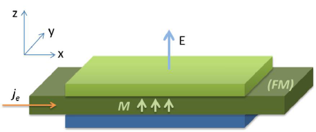
Figure 1: Schematic diagram of a ferromagnetic (FM) layer sandwiched between two dissimilar materials (oxides or heavy elements) to increase the vertical electric field $E_{z}$ and thus enhance the Rashba SOC effect. Current $\bm{j}_{e}$ flows in the in-plane $x$-direction. The magnetization of the FM layer $\bm{M}$ is oriented in the vertical $z$-direction.

The structure under consideration is depicted in Fig. 1. It consists of a metallic FM layer, sandwiched between two dissimilar materials (oxides or heavy elements) to enhance the RSOC interaction at the interfaces and within the FM layer. The local magnetization $\bm{M}$ is oriented along the vertical $z$-direction. A charge current $\bm{\hat{j}}_{e}$ is injected in the $x$-direction, which generates a field $H_{\mathrm{eff}}$ along the $\bm{\hat{y}}=(\bm{\hat{z}}\times\bm{\hat{j}}_{e}$) direction. The Hamiltonian for the system can be expressed as:

$$\hat{H} =\hat{H}_{0}+\hat{H}_{so},$$ (1)

$$\hat{H}_{0} =\frac{\hat{\bm{p}}^{2}}{2m}-\Delta({\bm{M}}\cdot\bm{\hat{S}}),$$ (2)

$$\hat{H}_{so} =\frac{\alpha_{R}}{\hbar}(\hat{\bm{p}}\times\hat{\bm{z}})\cdot\hat{\bm{S}},$$ (3)

where $m$ is the free electron mass, and $\hbar$ is the reduced Planck’s constant. Here, $H_{0}$ denotes the kinetic energy of the conduction electrons in the FM layer, ${\bm{M}}$ is the magnetization direction, $\Delta$ is the exchange coupling between the free electron spin and the local moments, and $\hat{\bm{S}}=\{\hat{S}_{j}\}$ (where $j=\{x,y,z\}$) is the vector of Pauli spin matrices. $\hat{H}_{so}$ denotes the Rashba interaction which couples the electron spin with its momentum, with $\hat{\bm{p}}$ being the electron momentum, and the potential gradient inducing the RSOC effect being assumed to be in the direction $\bm{z}$ normal to the FM layer. The potential gradient may arise from a variety of sources such as impurities, host atoms, and structural confinement sih.nat1 ; kim.apl012504 ; szunyogh.prl96 ; castro.prl103 ; matos.prb81 . In order to apply the many-body NEGF formalism, the above Hamiltonian has to be recast into the second quantized form:

$$\hat{H}_{0} =-t_{0}\sum_{\bm{r},\sigma}\sum_{\pm}c^{{\dagger}}_{\bm{r}\sigma}(c_{\bm{r}\pm\bm{a}\sigma}+c_{\bm{r}\pm\bm{b}\sigma})+\sum_{\bm{r},\sigma}\varepsilon_{\bm{r}\sigma}c^{{\dagger}}_{\bm{r}\sigma}c_{\bm{r}\sigma}$$ (4)

$$\hat{H}_{so} =-it_{SO}\sum_{\bm{r},\sigma,\sigma^{\prime}}\sum_{\pm}c^{{\dagger}}_{\bm{r}\sigma}(\pm(\hat{S}_{x})_{\sigma\sigma^{\prime}}c_{\bm{r}\pm\bm{b}\sigma^{\prime}}\mp(\hat{S}_{y})_{\sigma\sigma^{\prime}}c_{\bm{r}\pm\bm{a}\sigma^{\prime}}).$$ (5)

where $c_{\bm{r}\sigma}$($c_{\bm{r}\sigma}^{{\dagger}}$) is the fermionic annihilation(creation) operator of an electron with spin $\sigma=\uparrow,\downarrow$ at position $\bm{r}$. Here, $a$ is the lattice spacing representation on a square lattice in the tight-binding NEGF formulation , $\bm{a}=a\bm{e}_{x}$ and $\bm{b}=a\bm{e}_{y}$ are the unit lattice vectors. $t_{0}$ represents the hopping energy between lattice points, and is obtained by $t_{0}=\hbar/2ma^{2}$. The terms $\varepsilon_{\bm{r}\uparrow}=4t_{0}+\Delta/2$ and $\varepsilon_{\bm{r}\downarrow}=4t_{0}-\Delta/2$ represent the on-site energy at the lattice site, and $t_{SO}=\alpha_{R}/2a$ is the SO coupling energy due to the Rashba interaction.

In order to perform numerical analysis through the NEGF, the retarded ($G^{r}$) and lesser ($G^{<}$) Green’s functions are required. These are defined as

$$G^{r}_{\bm{r}\sigma,\bm{r}^{\prime}\sigma^{\prime}}(t,t^{\prime}) =i\langle\{c_{\bm{r}\sigma}(t),c^{{\dagger}}_{\bm{r^{\prime}}\sigma^{\prime}}(t^{\prime})\}\rangle\theta(t-t^{\prime}),$$ (6)

$$G^{<}_{\bm{r}\sigma,\bm{r}^{\prime}\sigma^{\prime}}(t,t^{\prime}) =i\langle c^{{\dagger}}_{\bm{r^{\prime}}\sigma^{\prime}}(t^{\prime})c_{\bm{r}\sigma}(t)\rangle$$ (7)

After Fourier transformation, the expression for $G^{r}$ in energy space is given by

$$G^{r}(\epsilon) =[\epsilon-\hat{H}-\Sigma^{r}(\epsilon)]^{-1}.$$ (8)

In the above, $\Sigma^{r}=\sum_{\alpha}\Sigma_{\alpha}^{r}$ is the retarded self-energy incurred by the lead $\alpha$, where $\alpha=L(R)$ represents the left (right) lead. $\Sigma_{\alpha}^{r}$ can be determined by $\Sigma_{\alpha}^{r}=V_{\alpha}g_{\alpha}^{r}V^{\dagger}_{\alpha}$, where $V_{\alpha}$ is the coupling matrix between the lead $\alpha$ and the FM layer, and $g_{\alpha}^{r}$ is the retarded Green’s function of the lead $\alpha$ and can be calculated numerically by the renormalization method nikolic:prb73 . $G^{<}$ can be calculated from the relation

$$G^{<}(\epsilon) =G^{r}(\epsilon)\Sigma^{<}(\epsilon)G^{a}(\epsilon).$$ (9)

where $G^{a}=(G^{r})^{{\dagger}}$. $\Sigma^{<}=\sum_{\alpha}\Sigma_{\alpha}^{<}$, where $\Sigma_{\alpha}^{<}=if_{\alpha}\Gamma_{\alpha}$ is the lesser self-energy due to lead $\alpha$, $f_{\alpha}$ is the Fermi function in lead $\alpha$, and $\Gamma_{\alpha}=-2$Im$\Sigma^{r}_{\alpha}$ is the linewidth function representing the coupling between the lead $\alpha$ and the central FM region.

Various transport properties can be evaluated once the different Green’s functions ($G^{r}$, $G^{a}$, and $G^{<}$) have been solved via Eqs. (8) and (9). The charge current through the system can be expressed in terms of the different Green’s functions, as follows

$$I_{\alpha}= \frac{e}{h}\int^{+\infty}_{-\infty}d\epsilon\medspace\mathrm{Tr}\left\{\left[\Sigma^{<}_{\alpha}(\epsilon)A(\epsilon)\right]-\left[\Gamma(\epsilon)_{\alpha}G^{<}(\epsilon)\right]\right\},$$ (10)

where $A(\epsilon)=i[G^{r}(\epsilon)-G^{a}(\epsilon)]$ is spectral function. Likewise, the current-driven local spin density in the central region is related to $G^{<}$ as follows

$$\langle s_{i}\rangle_{m} =\frac{\hbar}{2}\sum_{\sigma\sigma^{\prime}}(\hat{S}_{i})_{\sigma\sigma^{\prime}}\langle\hat{c}^{\dagger}_{m\sigma}\hat{c}_{m\sigma^{\prime}}\rangle$$

$$=\frac{\hbar}{4\pi i}\int^{\infty}_{-\infty}d\epsilon\sum_{\sigma\sigma^{\prime}}(\hat{S}_{i})_{\sigma\sigma^{\prime}}G^{<}_{mm,\sigma\sigma^{\prime}}(\epsilon),$$

$$=\frac{\hbar}{4\pi i}\int^{\infty}_{-\infty}d\epsilon\medspace\mathrm{Tr}[\hat{S}_{i}G^{<}_{mm}(\epsilon)],$$ (11)

where the subscript $m$ refers to the site index.

The spin torque exerted on the local magnetization can be defined as the difference between spin current going into and coiming out of the lattice point. We express the spin torque as the divergence of spin currentsalahuddin:arxiv :

$${\bm{\tau}} =\mu_{B}\int dV\nabla\cdot\bm{j}^{S_{i}},$$ (12)

where $V$ is the volume, $\mu_{B}$ is the Bohr magneton, and $\bm{j}^{S_{i}}$ is the spin current density between lattice points. The spin torque ${\bm{\tau}}$ can be also be defined as $\bm{\tau}=-\gamma\bm{M}\times{\bm{H}}$, where $\gamma$ is the gyromagnetic ratio. We focus on the effective field $H_{\mathrm{eff}}$ induced by Rashba SOC which acts on the local moments along the $\bm{\hat{y}}=(\bm{\hat{z}}\times\bm{\hat{j}}_{e}$) direction. Thus, the effective field due to RSOC is

$$H_{\mathrm{eff}} =H_{y}=\frac{\tau_{x}}{\gamma M_{s}V},$$ (13)

where $M_{s}$ is the saturation magnetization, and $\tau_{x}$ is obtained from Eq. (12). The torque efficiency is then given by ratio of $H_{\mathrm{eff}}/{j}_{e}$.

Under steady-state condition and in the absence of dissipative processes, the spin torque ${\bm{\tau}}$, as defined according to Eq. (12), is related to the divergence of the spin current. By considering the Heisenberg equation of motion, the local spin bond current between sites $m$ and $m^{\prime}$ can be expressed in terms of $G^{<}$ nikolic:prb73 ; hattori:JPSJ78 , i.e.

$$\langle\hat{j}^{s_{i}}_{mm^{\prime}}\rangle =\langle\hat{j}^{s_{i}(kin)}_{mm^{\prime}}\rangle+\langle\hat{j}^{s_{i}(SO)}_{mm^{\prime}}\rangle,$$

$$\langle\hat{j}^{s_{i(kin)}}_{mm^{\prime}}\rangle =\frac{et_{0}}{2\hbar}\int^{\infty}_{-\infty}\frac{d\epsilon}{2\pi}\medspace\mathrm{Tr}[\hat{S}_{i}(G^{<}_{m^{\prime}m}(\epsilon)-G^{<}_{mm^{\prime}}(\epsilon))]$$

$$\langle\hat{j}^{s_{i(SO)}}_{mm^{\prime}}\rangle =[\bm{e}_{i}\times(\bm{m^{\prime}}-\bm{m})]_{z}\frac{et_{SO}}{2\hbar}\int^{\infty}_{-\infty}\frac{d\epsilon}{2\pi i}\medspace\mathrm{Tr}[(G^{<}_{m^{\prime}m}(\epsilon)+G^{<}_{mm^{\prime}}(\epsilon))],$$ (14)

where $(\bm{m^{\prime}}-\bm{m})$ represents the unit vector between neighbouring sites on the $x$-$y$ plane and $\bm{e}_{i}$ represents the unit vector of spin $\langle S_{i}\rangle$. The above expression for the bond spin current comprises of two terms, i.e., the kinetic and SO coupling terms, arising from the corresponding terms in the Hamiltonian of Eqs. (2) and (3). By considering Eqs. (12) and (14) together, the spin torque is then given by the divergence of the spin bond current $(\nabla\cdot\bm{j}^{s})$, which in the discretized tight-binding model is approximated as:nikolic:prb73 ; hattori:JPSJ78

$$\tau_{x(\bm{m})} =-\mu_{B}\left(\langle\hat{j}^{s_{z}}_{\bm{m},\bm{m}+\bm{e}_{x}}\rangle+\langle\hat{j}^{s_{z}}_{\bm{m}-\bm{e}_{x},\bm{m}}\rangle\right)/L_{SO},$$ (15)

$$\tau_{y(\bm{m})} =-\mu_{B}\left(\langle\hat{j}^{s_{z}}_{\bm{m},\bm{m}+\bm{e}_{y}}\rangle+\langle\hat{j}^{s_{z}}_{\bm{m}-\bm{e}_{y},\bm{m}}\rangle\right)/L_{SO},$$ (16)

$$\tau_{z(\bm{m})} =\mu_{B}\left(\langle\hat{j}^{s_{x}}_{\bm{m},\bm{m}+\bm{e}_{x}}\rangle+\langle\hat{j}^{s_{x}}_{\bm{m}-\bm{e}_{x},\bm{m}}\rangle+\langle\hat{j}^{s_{y}}_{\bm{m},\bm{m}+\bm{e}_{y}}\rangle+\langle\hat{j}^{s_{y}}_{\bm{m}-\bm{e}_{y},\bm{m}}\rangle\right)/L_{SO},$$ (17)

where $L_{SO}$ is the spin precession length (over which spin precesses by 1 radian), and can be expressed as $L_{SO}=\frac{\pi at_{0}}{2t_{SO}}$. The above constitutes to the spin torque expression of Eq. (12).

III Results and Discussion

Based on the tight-binding NEGF formulation presented in the above section, we performed numerical calculations of transport parameters such as the local spin density, bond spin current, and the effective field $H_{\mathrm{eff}}$ in order to analyze the effect of RSOC induced non-equilibrium spatial spin torque on the FM layer structure. In our calculations, the following parameter values are assumed, unless otherwise stated: $\alpha_{R}=10^{-11}~{}\mathrm{eVm}$, $m=9.1\times 10^{-31}$ kg, $a=0.05~{}\mathrm{nm}$, $E_{F}=7.83~{}\mathrm{eV}$, $M_{s}=1.09\times 10^{6}~{}\mathrm{Am^{-1}}$, $\Delta=1.6~{}\mathrm{eV}$ Miranda.surf117 , and room temperature $T=300$ K. The Fermi energy $E_{F}$ and saturation magnetization $M_{s}$ assume exemplary values corresponding to that of Co.

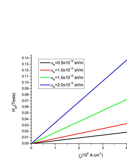
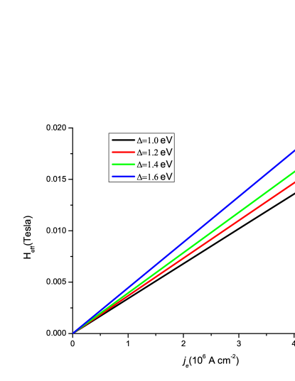
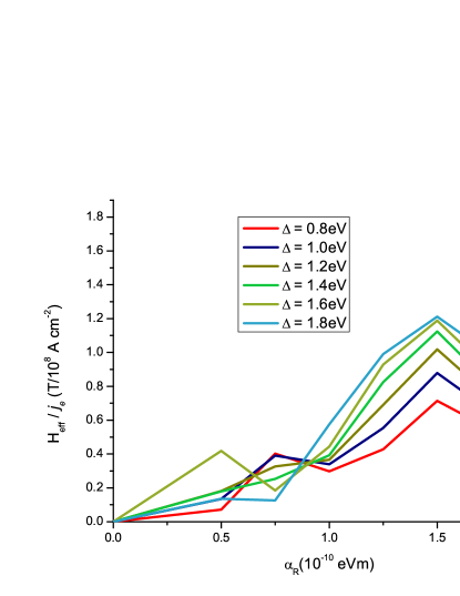
Figure 2: The dependence of the effective current induced field ($H_{\mathrm{eff}}$) due to the Rashba spin torque is plotted as a function of charge current density (${j}_{e}$) for (a) varying Rashba strength $\alpha_{R}$ with a fixed exchange coupling $\Delta=1.6$ eV, and (b) varying exchange coupling $\Delta$ with a fixed $\alpha_{R}=10^{-10}$ eVm. In (c), the spin torque efficiency ($H_{\mathrm{eff}}/j_{e}$) is plotted as a function of both $\Delta$ and $\alpha_{R}$. In the calculations, we assume the dimension of the sample to be $50a\times 50a$, where $a=0.05$ nm.

We first analyze the role of two key parameters $\alpha_{R}$ and $\Delta$ in determining the strength of the effective field $H_{\mathrm{eff}}$ and the torque efficiency of the system. Figs. 2 and 2 show that, with a fixed $\alpha_{R}$ and $\Delta$ respectively, $H_{\mathrm{eff}}$ increases linearly with $j_{e}$. This trend is consistent with the prediction that

$$H_{\mathrm{eff}}=\frac{\alpha_{R}P}{\mu_{0}\mu_{B}}(\hat{\bm{z}}\times\bm{j}_{e}),$$ (18)

derived from either gauge formulation tan:annal326 or from semiclassical (Boltzmann) transport equation manchon:prb78 in the strong coupling limit. Eq. (18) is a global expression of spin torque under linear response. In the gauge formulation, the factor $P$ assumes a value of $\frac{1}{2}$ in the adiabatic limit, while in the Boltzmann model, it refers to the spin polarization of current. We now consider the torque efficiency, which is given by the gradient of $H_{\mathrm{eff}}$ with respect to $j_{e}$. As can be seen from Figs. 2 and 2, the torque efficiency is generally enhanced with increase in either $\alpha_{R}$ and $\Delta$. However, in our non-equilibrium spatial treatment, it is clear from the plot in Fig. 2 that the torque efficiency does not vary linearly with $\alpha_{R}$, unlike the prediction of Eq. (18). The difference can be accounted for by noting that the global expression of Eq. (18) is derived in the limit of large coupling $\Delta$, i.e., up to only the linear order in $\frac{\alpha_{R}}{\Delta}$. In our model, as can be seen from Fig. 2, the torque efficiency shows a slight oscillatory dependence superimposed upon a general increase with respect to $\alpha_{R}$, especially at the region of $\alpha_{R}<10^{-10}$ eVm. However, at the region where $\alpha_{R}\geq 10^{-10}$ eVm, its behavior is similar to the prediction derived from the Boltzmann semiclassical model for arbitrary coupling strength manchon:prb78 . From the effective field $H_{\mathrm{eff}}$, one can estimate the critical current density required for magnetization switching. In Figs. 2 and 2, we consider RSOC strengths ranging from $10^{-11}$ to $10^{-10}$ eVm, which roughly corresponds to the practical values observed at the interfaces with heavy metal or oxide layers. Assuming an exemplary spin polarization of $P=\frac{\Delta}{E_{F}}\approx 0.5$, RSOC strength of $\alpha_{R}=10^{-10}$ eVm, and a switching field of $H_{s}\approx 0.02$ T applicable for Co nanowire structures mihai:natm9 , we find that the critical current density for switching is approximately $10^{6}$ A/$\mathrm{cm}^{2}$ [see Fig. 2]. This is significantly lower than the critical current density of the order of $10^{7}$ A/$\mathrm{cm}^{2}$ for the case of the conventional Slonczewski spin torque in spin valve structures jiang:prl92 ; sukegawa:apl96 .

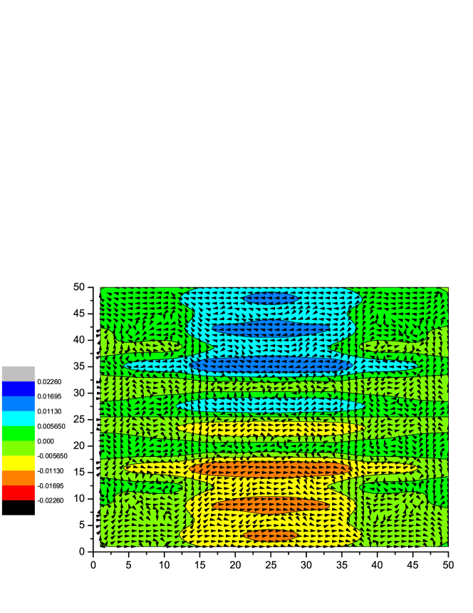
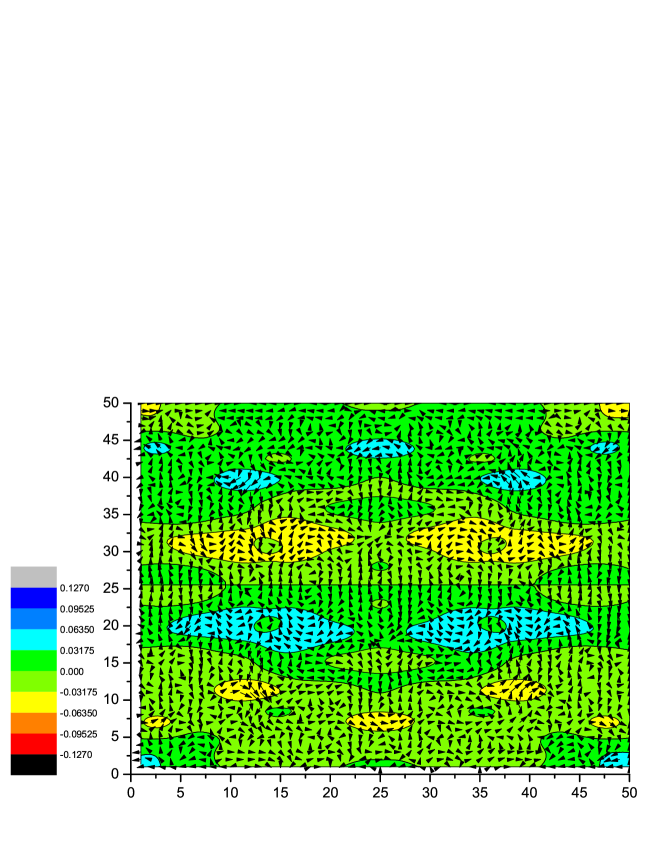
Figure 3: The spatial distribution of the (a) Rashba effect spin torque $\tau_{x}$ and its correlation with the local spin current $\langle j^{s_{z}}_{mm^{\prime}}\rangle$ by setting $\alpha_{R}$ to $0.5\times 10^{-10}$ eVm, (b) $\tau_{x}$ and its correlation with $\langle j^{s_{z}}_{mm^{\prime}}\rangle$ by setting $\alpha_{R}$ to $1.5\times 10^{-10}$ eVm. The spin torque density is expressed in units of $\mu_{B}/L_{SO}$. The sample has a lateral size of $50a\times 50a$.

Next, we examine the relationship between the Rashba-induced torque $\tau$ and the spatial distribution of the spin currents. In Fig. 3, we plot the spin torque component $\tau_{x}$ based on the torque definition of Eq. (15), which relates it to the divergence of the local spin bond current $j^{s_{z}}_{mm^{\prime}}$. For comparison, we plot the spatial distribution of the spin bond current $j^{s_{z}}_{mm^{\prime}}$ in Fig. 3. We observe a close correlation between the spatial distribution of $\tau_{x}$ and the flow of the $z$-polarized spin current $j^{s_{z}}_{mm^{\prime}}$. The presence of RSOC causes a vortex-like flow of the bond spin current $j^{s_{z}}_{mm^{\prime}}$ as shown in Fig. 3. Regions where $j^{s_{z}}_{mm^{\prime}}$ is flowing in the $+x$ ($-x$) direction corresponds to a large positve (negative) $\tau_{x}$. Conversely, in regions where the positive and negative spin current fluxes meet and cancel each other, the spin torque $\tau_{x}$ becomes small. When the Rashba coupling strength $\alpha_{R}$ is increased, the magnitude of $\tau_{x}$ is generally larger since it scales with $\alpha_{R}$, as shown in Fig. 2. In addition, the vortices associated with the spin current become spatially smaller. This may be attributed to the increase in the rate of spin precession of the conduction electrons with $\alpha_{R}$. The increased density of the vortices result in some cancelation of the bond spin currents near the center of the FM layer, so that more of the bond spin current flows at the boundaries, as shown in Fig. 3.

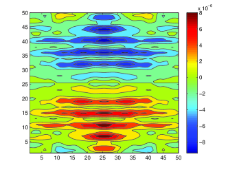
(a) $\Delta=0$, $\alpha_{R}=10^{-10}$ eVm, $\langle s_{z}\rangle_{m}$. SHE recovered.

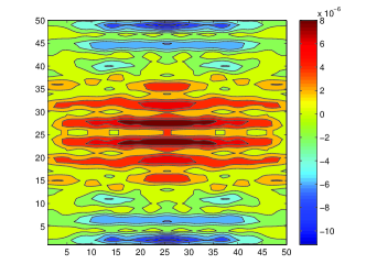
(b) $\Delta=0$, $\alpha_{R}=10^{-10}$ eVm, $\langle s_{y}\rangle_{m}$. Absence of SHE.

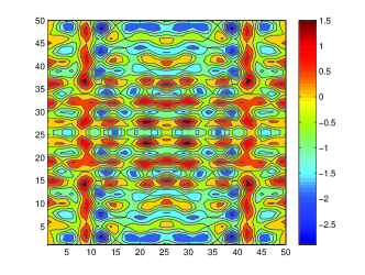
(c) $\Delta=1.6$ eV, $\alpha_{R}=5\times 10^{-11}$ eVm, $\langle s_{z}\rangle_{m}$. SHE disrupted

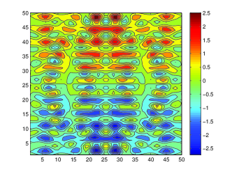
(d) $\Delta=1.6$ eV, $\alpha_{R}=5\times 10^{-11}$ eVm, $\langle s_{y}\rangle_{m}$. SHE detecteded.

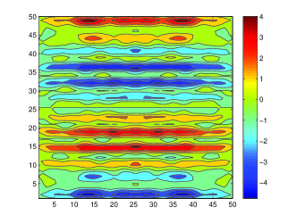
(e) $\Delta=1.6$ eV, $\alpha_{R}=1.5\times 10^{-10}$ eVm, $\langle s_{y}\rangle_{m}$. SHE disrupted.

Figure 4: The spatial distribution of the spin density (a) $\langle s_{z}\rangle_{m}$, (b) $\langle s_{y}\rangle_{m}$, both with $\Delta=0$ eV, $\alpha_{R}=1\times 10^{-10}$ eVm, (c) $\langle s_{z}\rangle_{m}$, (d) $\langle s_{y}\rangle_{m}$, both with $\Delta=1.6$ eV, $\alpha_{R}=1.5\times 10^{-10}$ eVm. In (e) $\langle s_{y}\rangle_{m}$ is plotted with a larger $\alpha_{R}=1.5\times 10^{-10}$ eVm, and $\Delta=1.6$ eV. The sample has a lateral size of $50a\times 50a$.

Finally, we analyze the spin density distribution and its dependence on the exchange strength $\Delta$. Figs. 4(a) and 4(b) plot the spin density of $\langle s_{z}\rangle_{m}$ in the absence and presence of $\Delta$, respectively. In the absence of exchange coupling ($\Delta=0$), the distribution profile of $\langle s_{z}\rangle_{m}$ clearly indicates a transverse separation of the $z$-spins, i.e. an out-of-plane spin Hall effect. This agrees with previous calculations based on the multimode scattering matrix method which predict a spin-Hall like separation of the out-of-plane spin component in the presence of Rashba effect brusheim:prb74 . However, the clear out-of-plane spin Hall separation disappears when a sizable exchange $\Delta$ is present, as shown in Fig. 4(c). It is found that the magnitude of $\langle s_{z}\rangle_{m}$ assumes a much larger value throughout the FM layer. This increase may be attributed to the alignment of the electron spin to the local moments oriented along the $z$-direction. We also analyze the in-plane spin density $\langle s_{y}\rangle_{m}$ distribution, as shown in Figs. 4(b), 4(d), and 4(e). There is no transverse separation of the in-plane spin density in the absence of $\Delta$ [Fig. 4(b)]. This is in line with theoretical prediction where the spin Hall effect induced by RSOC applies only to out-of-plane spins. However, in the presence of strong exchange coupling $\Delta$, an “in-plane” spin Hall effect is present [Fig. 4(d)]. This in-plane spin Hall effect is destroyed in the presence of a strong Rashba strength, i.e. when $\alpha_{R}$ is increased to $1.5\times 10^{-10}$ eVm [Fig. 4(e)]. This may be explained by noting that a large RSOC strength increases the rate of spin precession. Thus, the in-plane spin density $\langle s_{y}\rangle_{m}$ oscillates and changes signs along the direction of electron propagation ($x$-direction), as can be seen in Fig. 4(d).

IV Conclusion

In summary, we have studied the non-equilibrium spatial intrinsic spin torque induced by Rashba spin orbit coupling in a ferromagnetic metal layer. Unlike the conventional Slonczewski spin torque, the Rashba induced torque is generated within a single layer, i.e. it does not require spin injection from an another ferromagnetic reference layer. We analyze the effect of two crucial parameters determining the strength of the Rashba spin torque: (i) the strength $\alpha_{R}$ of the RSOC effect which is responsible for polarizing the injected charge current, and (ii) the exchange splitting $\Delta$ which couples the conduction electron to the local FM moments, thus allowing the transfer of spin momentum to the latter. The spin transport through the system is modeled via the tight-binding non-equilibrum Green’s function (NEGF) formalism. The NEGF theory systematically incorporates many-body effects including interactions with the leads as self-energy terms, and enables current and spin density to be evaluated spatially under nonequilibrium (bias-driven) conditions. Based on the NEGF theory, we numerically evaluate various transport parameters of the system, such as the effective field $H_{\mathrm{eff}}$ due to the spin torque, and the spatial distribution of the non-equilibrium spin current and spin accumulation. We found that $H_{\mathrm{eff}}$ generally increases with both the RSOC strength $\alpha_{R}$ and the exchange coupling $\Delta$. However, the dependence of $H_{\mathrm{eff}}$ on both parameters is not totally linear, unlike previous predictions based on gauge formulation or semiclassical Boltzmann which are global and only partially non-equilibrium (linear response), and in the strong coupling limits. For practical values of $\Delta$ and $\alpha_{R}$, the calculated critical current density corresponding to a typical switching field of 200 mT is calculated to be lower than $10^{7}$ A/$\mathrm{cm}^{2}$, comparable to that obtained via the conventional Slonczewski spin torque. For the structure under consideration where net current is in the $x$-direction and the local moments are aligned in the vertical $z$-direction, the net effective field (spin torque) is in the $y$ ($x$)-direction. We plot the spatial profile of the $x$-component of the spin torque $\tau_{x}$, which bears a close correlation to that of the $z$-polarized bond spin current. It is also observed that the Rashba torque $\tau_{x}$ is concentrated near the boundaries of the FM layer. We also found that the combined presence of RSOC effect and exchange coupling $\Delta$ induces a Hall separation of in-plane spins, whereas the spin Hall effect for out-of-plane spins disappear with the introduction of $\Delta$. Our calculations predict an effective field $H_{\mathrm{eff}}$ of the order of 1 Tesla for a current density of $10^{7}$ $\mathrm{A/cm}^{2}$, thus indicating the feasibility of utilizing the Rashba induced spin torque to achieve magnetization switching in spintronic applications.

References

- (1) J. C. Slonczewski, J. Magn. Magn. Mater. 159, L1 (1996).
- (2) L. Berger, Phys. Rev. B 54, 9353 (1996).
- (3) J. A. Katine, F. J. Albert, R. A. Buhrman, E. B. Myers, and D. C. Ralph, Phys. Rev. Lett. 84, 3149 (2000).
- (4) Y. Huai, F. Albert, P. Nguyen, M. Pakala, and T. Valet, Appl. Phys. Lett. 84, 3118 (2004).
- (5) K. Obata and G. Tatara, Phys. Rev. B 77, 214429 (2008).
- (6) S. G. Tan, M. B. A. Jalil, T. Fujita, and X.-J. Liu, Ann. Phys. 326, 207 (2011), (S. G. Tan and M. B. A. Jalil and X-J Liu[arXiv:0705.3502v1]).
- (7) A. Manchon and S. Zhang, Phys. Rev. B 78, 212405 (2008).
- (8) I. Mihai Miron et al., Nat. Mater. 9, 230 (2010).
- (9) U. H. Pi et al., Appl. Phys. Lett. 97, 162507 (2010).
- (10) J. B. Miller et al., Phys. Rev. Lett. 90, 076807 (2003).
- (11) Y. Sato, T. Kita, S. Gozu, and S. Yamada, J. Appl. Phys. 89, 8017 (2001).
- (12) S. Giglberger et al., Phys. Rev. B 75, 035327 (2007).
- (13) A. V. Larionov and L. E. Golub, Phys. Rev. B 78, 033302 (2008).
- (14) M. Akabori et al., Phys. Rev. B 77, 205320 (2008).
- (15) S. LaShell, B. A. McDougall, and E. Jensen, Phys. Rev. Lett. 77, 3419 (1996).
- (16) C. R. Ast et al., Phys. Rev. Lett. 98, 186807 (2007).
- (17) H. Cercellier et al., Phys. Rev. B 73, 195413 (2006).
- (18) O. Krupin et al., Phys. Rev. B 71, 201403 (2005).
- (19) J. Premper, M. Trautmann, J. Henk, and P. Bruno, Phys. Rev. B 76, 073310 (2007).
- (20) C. R. Ast et al., Phys. Rev. B 77, 081407 (2008).
- (21) S. Abdelouahed and J. Henk, Phys. Rev. B 82, 193411 (2010).
- (22) J. H. Dil et al., Phys. Rev. Lett. 101, 266802 (2008).
- (23) V. Sih et al., Nat. Phys. 1, 31 (2005).
- (24) K.-H. Kim, H. jun Kim, H. C. Koo, J. Chang, and S.-H. Han, Appl. Phys. Lett. 97, 012504 (2010).
- (25) L. Szunyogh, G. Zaránd, S. Gallego, M. C. Muñoz, and B. L. Györffy, Phys. Rev. Lett. 96, 067204 (2006).
- (26) A. H. Castro Neto and F. Guinea, Phys. Rev. Lett. 103, 026804 (2009).
- (27) A. Matos-Abiague, Phys. Rev. B 81, 165309 (2010).
- (28) B. K. Nikolić, L. P. Zârbo, and S. Souma, Phys. Rev. B 73, 075303 (2006).
- (29) S. Salahuddin, D. Datta, and S. Datta, (2008), arXiv:0811.3472v1.
- (30) K. Hattori, J. Phys. Soc. Jpn 78, 084703 (2009).
- (31) R. Miranda, F. Yndurán, D. Chandesris, J. Lecante, and Y. Petroff, Surface Science 117, 319 (1982).
- (32) Y. Jiang et al., Phys. Rev. Lett. 92, 167204 (2004).
- (33) H. Sukegawa, S. Kasai, T. Furubayashi, S. Mitani, and K. Inomata, Appl. Phys. Lett. 96, 042508 (2010).
- (34) P. Brusheim and H. Q. Xu, Phys. Rev. B 74, 205307 (2006).