Markov models for fMRI correlation structure: is brain functional connectivity small world, or decomposable into networks?
Abstract
Correlations in the signal observed via functional Magnetic Resonance Imaging (fMRI), are expected to reveal the interactions in the underlying neural populations through hemodynamic response. In particular, they highlight distributed set of mutually correlated regions that correspond to brain networks related to different cognitive functions. Yet graph-theoretical studies of neural connections give a different picture: that of a highly integrated system with small-world properties: local clustering but with short pathways across the complete structure. We examine the conditional independence properties of the fMRI signal, i.e. its Markov structure, to find realistic assumptions on the connectivity structure that are required to explain the observed functional connectivity. In particular we seek a decomposition of the Markov structure into segregated functional networks using decomposable graphs: a set of strongly-connected and partially overlapping cliques. We introduce a new method to efficiently extract such cliques on a large, strongly-connected graph. We compare methods learning different graph structures from functional connectivity by testing the goodness of fit of the model they learn on new data. We find that summarizing the structure as strongly-connected networks can give a good description only for very large and overlapping networks. These results highlight that Markov models are good tools to identify the structure of brain connectivity from fMRI signals, but for this purpose they must reflect the small-world properties of the underlying neural systems.
keywords:
fMRI , brain networks , small-world , functional connectivity , Markov models , decomposable graphs1 Introduction
The study of distant correlations in functional Magnetic Resonance Imaging (fMRI) signals, revealing brain functional connectivity, has opened the door to fundamental insights on the functional architecture of the brain [1, 2]. Among other features, the concept of cognitive network has emerged as one of the leading views in current cognitive neuroscientific studies: regions that activate together form an integrated network corresponding to a cognitive function [1]. In other words, these networks can in general be identified to sets of active regions observed in traditional brain mapping experiments, thus in line with a segregative view of brain functional organization. On the other hand, graph-theoretical analysis of brain connectivity has shown that it displays small-world properties: any two points of the brain can be connected through few intermediate steps, despite the fact that most nodes maintain only a few direct connections [2]. There is an apparent contradiction between those two points of views: can the brain be separated in functionally-specialized networks, or are these simply a convenient but misleading representation to interpret the data?
Establishing a link between the functional connectivity observed in fMRI and the underlying neural architecture can be a challenging task. Indeed, the fMRI signal is very noisy and reflects many non neural effects, such as cardiac and respiratory rhythms or head and body motion. In addition, statistical estimation of brain interactions from fMRI data is made difficult by the small number of observations available per experimental run, and by the lack of salient structure in this data. Finally, it has become a common practice to study these interactions during resting-state, i.e. in the absence of any stimulation, the subject resting eyes-closed in the scanner; in that case functional connectivity is loosely identified with the correlation structure of ongoing activity across regions.
In this paper, we use advanced statistical techniques to investigate the structure of brain connections that is captured by resting-state fMRI recordings. For this purpose, we infer the Markov network structure of the signals –the underlying independence graph– using a statistical framework well suited to modeling correlations: Gaussian graphical models. We compare various estimation methods adapted to different graph topologies. In particular, we introduce decomposable Markov models to describe functional networks: sets of distant regions working together. Importantly these tools enable to study the extent –i.e. the clique size– of brain functional networks that is required to give a good description of the signal. Our work introduces a probabilistic description of brain activity that encompasses features of distributed cognitive network and small-world systems.
The layout of the article is the following. First we review different pictures of brain connectivity emerging from a vast body of anatomical and structural studies. In section 3, we introduce the statistical tools that we use to estimate functional connectivity graphs from the fMRI signal. In section 4, a method for learning decomposable models of brain activity is presented. Finally, in section 5, we estimate graphical models of brain activity with various methods and quantify their ability to fit unseen data as a function of the imposed graph topology: a strong segregation into well-separated distributed networks, or a highly-connected system.
2 Brain structure: from small-world connectivity to functional networks
Integration and segregation in neural systems
Beyond the historical opposition of localizationist and holist views [3], brain organization is generally considered as reflecting the fundamental principles of segregation into functionally-specialized sub-systems, and integration across these systems to sustain high-level cognitive functions [4]. Originally highlighted in theoretical descriptions of neural systems [5], this general organization shapes the properties of brain-wide connectivity: local clustering and global connectivity [6, 2] that reflects functional integration [7]. In high-level cognition, it can been seen as the duality of local circuits and global networks [8], for instance in conscious information integration [9]. Finally, there is growing evidence from functional imaging, that this segregation increases during brain development [10, 11].
Small word graphs
A quantitative description of these structural properties can be given using graph theory. In mathematics and computer science, a graph is the abstract object defined by a set of nodes and their connections. In social sciences or neuroscience, the word “network” is often employed instead of “graph”, but in this paper, we will reserve this term to denote cognitive or functional networks. Watts and Strogatz [12] popularized the concept of small-world properties for graphs: graphs with a small fraction of nodes connected, but with a connection topology such that only a short chain is required to connect any pair of nodes. These efficient transport properties are achieved via a local clustering into communities, and a few edges interconnecting the communities across the graph. A graph can be characterized by a variety of statistical properties of its connections [13, 14, 2]. Most often, small-world graphs are studied via the relative importance of a local graph metric, such as their clustering coefficient, and a global metric, e.g. their average path length [12, 13, 15]. The fundamental characteristic of a small-world graph remains that it displays high sparsity and yet good transport across the graph. Watts and Strogatz [12] stress that, for sparse graphs, small-worldness is determined by its global properties: “at the local level (as reflected by [the clustering coefficient]), the transition to a small world is almost undetectable” while “in sparse networks with many vertices […] even a tiny fraction of short cuts would suffice”.
Graphs of brain connectivity
The physical connections between gray-matter areas can be measured in-vivo via tractography of diffusion MRI [16, 17]. They establish a picture of the human brain architecture at an anatomical-connectivity level [18, 19]. In non-human animals, systematic post-mortem studies have enabled detailed and complete mapping of connections, e.g. for the macaque brain [20, 21]. This anatomical connectivity forms the substrate of information processing in the brain and reflects the functional segregation properties of neural systems [22]. From the point of view of graph theory, it has been shown to display small-world properties [6, 2]. In fact, Watts and Strogatz [12] used the graph of neural connections of C. elegans in their seminal paper introducing small-world graphs. It is also possible to build graphs of functional connectivity by thresholding correlation matrices of brain activity, for instance from MEG [23] or fMRI data [24, 25, 26, 27]. As their anatomical counterparts, these have been shown to display small-world properties: local clustering and short average path length.
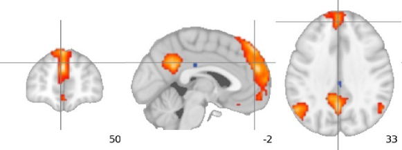 (a)
(a)
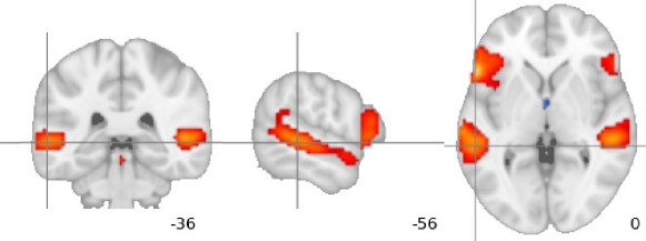 (b)
(b)
Intrinsic functional networks
The seminal work of Biswal et al. [30] showed that correlations in resting-state brain activity, i.e. in the absence of task, can be used to reveal brain systems dedicated to a cognitive function, often called intrinsic functional networks. Indeed, in the presence or in the absence of explicit cognitive task, a large fraction of brain activity is due to on-going functional processes. After Shulman et al. [31] used task-independent spatial correlations maps to uncover a new and important functional network [29], analysis of fluctuations in on-going activity has been used to systematically map the large-scale intrinsic functional architecture of the brain [1, 32]. Data-driven extraction of the main functional networks from resting-state data has been shown to be stable across subjects [33, 28]. These networks form a relevant description of the brain: they are found alike in on-going activity and in task-driven experiments, and stand out as landmark structures in meta-analyses carried out on current functional protocols [34]; they provide relevant descriptors for large scale pathologies such as neurodegenerative diseases [35]; and they reflect the underlying anatomical connectivity [36, 37]. An important aspect of these networks is that many correspond directly to set of regions that are specifically recruited for certain cognitive processes, including higher-order functions, such as language (Fig. 1.b) or executive function [38]. This decomposition of on-going activity offers a insightful view on the functional architecture of the brain, that is the interplay of a set of weakly-overlapping, functionally-specialized, brain networks: “the human brain is intrinsically organized into dynamic, anticorrelated functional networks” [39].
Criticism of small-world analyses
The analysis of brain architecture in terms of its graphical properties or its intrinsic functional networks gives differing points of view: on the one hand the distance on the connectivity graph between any two nodes of the small-world brain is small; on the other hand the brain appears as decomposed in functionally-specialized and weakly-overlapping networks of regions. While these two descriptions are not mutually exclusive, small-world analyses have drawn some criticism. Ioannides [40] criticizes the random-graph description of brain networks, as it is based on a small number of graph metrics that give a fairly unspecific characterization of the brain. He argues for a “hierarchy of networks rather than the single, binary networks that are currently in vogue”. More fundamentally, Ioannides raises the issue that these properties can easily be confounded by observation noise: “[in M/EEG] the activation of few (or many) uncorrelated generators will […] produce a small-world topology in a network computed from the raw signal topography” [40]. Indeed, Deuker et al. [41] find an inter-class correlation of less than 0.5 on the small-worldness index in a test-retest study using MEG for 2.5 minutes1112.5 minutes of acquisition time may seem short, yet for MEG, it provides orders of magnitude more observations than a standard fMRI experimental run of resting-state acquisition. In addition, simulation-based studies show that an observed small-world structure for a graph empirically derived from time-series may solely be explained by sampling effects [42, 43].
It is thus legitimate to ask whether the small-world properties of functional connectivity are indeed necessary to give a good description brain activity, or whether a picture of brain function in terms of separated cognitive networks is sufficient in view of the data.
3 Statistical tools for connectivity analysis: Markov and Gaussian graphical models
Notations
To clarify the mathematical presentation, we apply the following conventions. We write sets with capital letters, matrices with capital bold letters, , and we denote the operator norm, , and the norm, . is the identity matrix. Quantities estimated from the data at hand are written . is the matrix inverse of , is the transposed matrix. Finally, we write , for a symmetric matrix with strictly positive eigenvalues, i.e a positive definite matrix.
3.1 Probabilistic modeling of brain network structure
A limitation of the commonly used graph-theoretical descriptions of functional connectivity is that they do not form a probabilistic model of the functional signal. As such, they convey no natural notion of goodness of fit and hypothesis testing of the graph properties in the presence of noise is ill-defined. This is why we resort to the analysis of graphical models specifying a probability distribution for the signal. Namely we use Markov models, that we apply to the functional-connectivity correlation matrices in the framework of Gaussian graphical models.
Markov models: conditional independence graphs
Measures of functional connectivity are based on correlations in the BOLD signal. They cannot be easily interpreted in terms of transfer of information or effective connectivity, that is the influence that a neural system exerts over another [44]. Indeed, BOLD is a very indirect measure of neural firing, the MRI signal observed contains many non BOLD-related confounds, and correlation is a rough summary of the dependence between two variables revealing, amongst other things, indirect effects.
For these reasons, we focus our study on recovering the independence structure of the observed functional signals. With the data at hand, fMRI recordings with limited observations available, this is a challenging statistical estimation problem. We use a class of probabilistic models called Markov models that specify the independence structure of the variables that it describes. It can be represented as a graph, in which case a node is statistically independent from nodes to which it is not directly connected, conditionally on its neighbors.
In the context of brain functional connectivity, we are interested in inferring the graphical structure from the correlations in the observed activity. We frame this problem as estimating the Markov structure222More specifically, we learn a undirected graph of conditional independence. Such a model is often called a Markov Random Field model. of a Gaussian graphical model of brain activity.
Gaussian graphical models
The study of functional connectivity focuses on second-order statistics of the signal, in other word Gaussian statistics. While the underlying signals are most-likely not Gaussian, these measures have been shown to capture well the independence structure underlying fMRI signals [45]. A multivariate Gaussian model with a specified Markov structure is called a Gaussian graphical model [46]. We apply this class of models to the study of brain connectivity.
A centered Gaussian model is fully specified by the inverse of its covariance matrix, known as its precision matrix , that closely relates to conditional correlations between its variables. The conditional independence between variables in the model are given by the zeros in this matrix. Therefore the statistical estimation task that we are interested in, is to find these zeros in the precision matrix.
We start from a brain activation dataset with variables, the activation of different brain regions, and samples. We are interested in inferring a large-scale connectivity graph, that is between many nodes, from a comparatively small amount of observations. In these settings, estimating the covariance matrix, or the precision matrix, from the data is an ill-posed problem (see for instance [47, 48]). First, if , the number of unknown parameters is greater than the number of samples. Second, the various parameters to estimate are not mutually independent, as the estimated covariance has the constraint of being positive definite.
Thus, the Markov structure of the data cannot be estimated simply by thresholding the precision matrix. We resort to modern covariance estimation tools, namely covariance selection, as detailed below. In this context, specifying a Markov structure acts as a regularization for the covariance matrix estimation: it injects a prior information that a certain number of coefficients of the precision matrix are zero, and thus decreases the number of coefficients to be estimated.
Smith et al. [45] have shown on realistic simulations of brain functional connectivity that sparse -penalized inverse covariance estimators performed well to recover the graphical structure from noisy data. Huang et al. [49] and Varoquaux et al. [7] used such a sparse covariance estimation procedure to infer the conditional independence structure of a Gaussian graphical model on full brain data.
Assessing model fit
As a Gaussian graphical model defines a probability of observing data, its log-likelihood can be used as a natural metric for assessing the goodness of fit of the model for some test data : for a model specified by its precision matrix ,
| (1) |
where is the empirical covariance of the data: .
For our application, an important point is to separate properties of the functional connectivity networks extracted from the signal from features learned on observation noise particular to the experimental run. This problem is well known in statistics under the term of overfit. We use a standard technique to control overfit known as cross-validation: having learned a probabilistic model on a given set of experiment run, we test its goodness of fit on unseen data. Features learned by chance do not generalize to unseen data, as it is independent from the training data.
3.2 Covariance selection procedures
As proposed by Dempster [50], learning or setting conditional independence between variables can be used to improve the conditioning of an estimation problem, a technique referred to as covariance selection. Improved covariance estimation can therefore be achieved by estimating from the data a precision matrix with a sparse support, i.e., a small number of non-zero coefficients.
Selecting the non-zero coefficients to optimize the likelihood of the model given the data (eq. 1) is a difficult combinatorial optimization problem. It is NP hard in the number of edges and it therefore cannot be solved on moderately large graphs. To tackle such problems efficiently, two strategies coexist: convex relaxation approaches that lead to optimal solutions for a new problem that is a convex approximation of the initial problem and greedy approaches that find sub-optimal solutions.
Sparse penalized inverse covariance estimation
A constraint based on the number of non-zero coefficients leads to NP hard problems. It can be modified by replacing it by a constraint on the norm of the solution. This leads to a penalized estimator taking the form of the following convex optimization problem [51]:
| (2) |
where is the element-wise norm of the off-diagonal coefficients in the matrix. This problem can be solved very efficiently in time [52, 53]. This technique makes no assumption on the topology of the graph other than its sparsity. Its major limitation is that the penalty may bias the coefficients of the precision matrix. It was employed successful to learn functional connectivity graphs by Huang et al. [49] and Varoquaux et al. [7] on full-brain fMRI data, as well as Smith et al. [45] on realistic simulations of neural interactions.
PC-DAG
A greedy approach to learning the Markov independence structure of observed data is given by the PC algorithm [54]. It consists in pruning edges of a graph by successively testing for conditional independence. Although it does not solve a global optimization criteria, this algorithm is proved to be consistent [54, 55]. In the case of covariance selection, it can be used efficiently to learn a sparse precision matrix, as in the PC-DAG algorithm [56]: the PC algorithm is applied to estimate a Markov structure for the Gaussian graphical model, which is then used to estimate the precision matrix. An important point is that the Markov independence structure estimated is constructed as the moral graph333A moral graph of a directed graph is the equivalent undirected graph in terms of non-directed conditional independence relations [46] of the (possibly) directed conditional independence relation extracted by the PC algorithm. This graph is limited by the PC algorithm to a small node degree. This implies that the graphs extracted by the PC-DAG are unlikely to contain large cycles. This procedure is interesting because its computational cost scales exponentially with the maximum number of neighbors on the underlying graph, rather than the number of possible edges.
Shrinkage estimates
Finally, a more naive but quite efficient approach in practice consists in regularizing the estimate of the precision matrix by adding a diagonal matrix to the empirical covariance before computing its inverse. It amounts to an shrinkage by penalizing uniformly off-diagonal terms:
| (3) |
Ledoit and Wolf [47] have introduced a closed formula for a choice of leading to a good bias-variance compromise. Empirical results show that this method can achieve good generalization scores even with small sample sizes. The intuition behind this good performance is that a sample covariance matrix tends to over-estimate pair-wise correlations in the small-sample limit444Indeed the plug-in estimator for pair-wise correlations, , which also corresponds to the scaling of off-diagonal coefficients in the empirical covariance, is known to be biased at small samples. In particular, this bias implies that the most probably observed correlation is smaller than the population value, as discussed in [57] page 520.. Shrinking them to zero thus improves the estimate. This procedure gives a good baseline to compare goodness of fit of models, however, it does not extract a graph structure from the observed time series, as it does not set zeros in the precision matrix.
3.3 Decomposable graphical models
Here, we introduce the notion of decomposable graphs, and present some related properties interesting to describe brain functional networks.
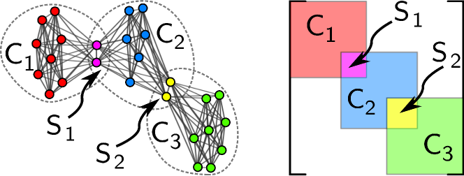
A graph is said to be chordal if each of its cycles of four or more nodes has a chord, i.e., an edge joining two nodes that are not adjacent in the cycle. A chordal graph can be divided in an ordered sequence of cliques555A clique is a fully-connected sub-graph: each nodes is connected to every other node. [46], as illustrated in Fig. 2. The intersection between two successive cliques and forms a complete subgraph666A complete graph is a graph in which all pairs of nodes are connected. called a separating set . When the structure of a graphical probabilistic model is chordal, the model is said to be decomposable [58]. The different cliques are then mutually independent conditionally on the separating set , and the likelihood factors in terms corresponding to the different cliques and separating sets:
| (4) |
where denotes the dataset reduced to the variables of clique and denotes the corresponding reduced precision matrix [46]. While there exists no closed formula for the Maximum Likelihood Estimate (MLE) of the precision matrix for an arbitrary sparse graphical Gaussian model, the MLE for a decomposable model can be written as:
| (5) |
where denotes the MLE for the precision matrix of the fully-connected subset of reduced to the clique , that is the inverse empirical covariance matrix, padded with zeros to the size of the full model [46]. Identifying the cliques and separating sets in a graphical model opens the door to an efficient estimation of the maximum-likelihood precision matrix. Note that a non-decomposable model can be turned in a decomposable model: cordless cliques can be completed to turn the graph in a chordal graph.
The motivation for using decomposable models to learn brain connectivity is twofold. First, the covariance matrices are estimated at the clique level, which are smaller problems. This strongly limits the estimation error. More importantly, the description of the brain that decomposable models give, cliques of regions that are mutually independent conditionally to set of hubs nodes, seems to match well the intuition of the functional networks composing brain architecture. Models sharing a similar intuition but not relying on a graphical description have been popularized in neuroimaging through the concept of integration of brain regions within a network [59].
4 Efficient learning of decomposable structures
In this section, we introduce a new algorithm to learn decomposable models on large covariance matrices without a priori knowledge of the relevant cliques. Indeed, to date, none of the standard covariance selection procedures for large-scale graphs seeks a decomposable model. While Bayesian approaches to learning Gaussian graphical models often rely on decomposable models, they require sampling of the space of models, and therefore are intractable on problems with more than a few dozen of nodes [60, 61]. Marlin and Murphy [62] recently proposed an algorithm to impose a clique structure on Gaussian graphical models. However, their approach, with an complexity, requires a known ordering of the nodes.
We propose a fast algorithm, that we call FastDecomp, to learn a decomposable graph with a large-scale structure common to several datasets. Our goal is to find a structure of conditional independence between successive blocks of variables. Our algorithm is based on a greedy approach to select non-independent variables.
The FastDecomp algorithm
Similarly to the PC-Algorithm, we start from a complete graph , compute pair-wise partial correlations conditioning on all other variables, and use them to test conditional independence between variable pairs to prune the graph. However, to keep bounds on the computational cost, we do not pursue to test conditional independence exhaustively. To test for independence between nodes and , conditioning on , we first test conditional independence using Fisher’s z-transform of the estimated partial correlation777We use the Ledoit-Wolf estimator to estimate the partial correlation, as it gives a good bias-variance compromise.:
| (6) |
has approximately a distribution if (see Rütimann and Bühlmann [56] for similar considerations).
Once all the pair-wise partial correlations are tested, we find a good completion of the resulting graph to a chordal graph888Finding the best possible chordal completion is know to be NP-hard [64].. For this we apply the symmetric Reverse Cuthill-McKee (RCM) algorithm [63] on the corresponding adjacency matrix to obtain a peripheral node999A peripheral node of a graph is a node for which the shortest path to another node is the diameter of the graph, that is the maximum shortest path between all nodes. The reverse Cuthill-McKee algorithm does not directly output a peripheral node, but we use its graph traversal and dynamical programming to find a pseudo peripheral node for little added cost. and an ordering minimizing the envelop of the graph. We start from the peripheral node and jump successively to the adjacent node furthest according to the RCM ordering, which gives us an enumeration of the cliques of the chordal graph, and the separating sets .
Finally, on each clique (resp. separating set ) we estimate the precision matrix by applying the Ledoit-Wolf estimator to the observed data, restricted to the clique (resp. separating set). We obtain the final precision matrix using formula 5. See listing 1 for a precise description of the algorithm.
Computational cost
The Reverse Cuthill-McKee can be implemented in [65]. The bottleneck of our algorithm is thus the last loop: calculating the precision on each clique and each separating set. The cost of this loop as bounded by times a matrix inversion. The FastDecomp algorithm is thus bounded by .
5 Experimental results: graphical models of on-going brain activity
5.1 A resting-state fMRI dataset
We apply the various covariance-selection methods to estimate the Markov independence structure from a resting-state fMRI dataset acquired in a previous experiment [66]. 12 subjects were scanned in a resting task, resulting in a set of 810 brain volumes per subject acquired with a repetition of 1.5 second. The data were preprocessed using the SPM5 software101010Wellcome Department of Cognitive Neurology; www.fil.ion.ucl.ac.uk/spm, including in particular the spatial normalization to standard template space. As in Achard et al. [25], or Huang et al. [49], we extract brain-activation time series on a parcellation of the gray matter in 105 non-overlapping regions111111The complete atlas comprises 110 regions, but as the field of view of our fMRI images is reduced, it does not cover the cerebellum.. As we are interested in modeling only gray-matter correlations, we regress out confound effects obtained by extracting signals in the white matter, the cortico-spinal fluid regions, as well as the rigid-body motion time courses estimated during data pre-processing.
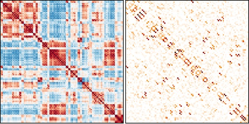
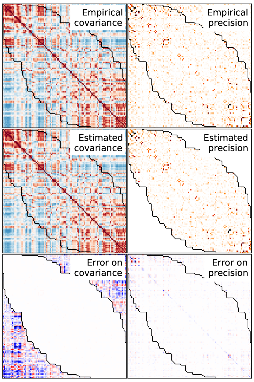
The correlation matrix of the resulting signals can be seen in Figure 3 (left). On this figure, regions are ordered according to the labels of the atlas that was used to define them [67]. This ordering groups together regions that belong to the same general bilateral anatomical structures. A first visual analysis reveals large blocks of correlated regions. This can be interpreted as the signature of the so-called cognitive networks.
The corresponding empirical precision matrix (Figure 3, right) reveals the partial correlations between regions. It appears more sparse; in particular the block-structure is not visible.
5.2 Generalization performance of the various estimators
We learn from this dataset different Gaussian graphical models of brain activity using the different covariance selection procedures: sparse penalized inverse covariance estimation121212We use an implementation of the -penalized inverse covariance estimator following Rothman et al. [68], PC-DAG, and FastDecomp. We evaluate the goodness of fit of the different models using a leave-one-out procedure: we learn a sparse precision on 11 subjects131313We apply the estimators on the concatenated individual data: , after detrending, band-pass filtering, and variance-normalizing the individual time series. The generative model underlying this concatenation corresponds to the hypothesis that all the different observations are drawn from the same distribution. It is a common assumption in unsupervised analysis of resting-state dataset, popularized with ICA [69]. and test the likelihood of the data corresponding to the subject in the model described by this precision matrix. In the likelihood term (eq. 1), we use correlation matrices, rather than covariances, as we are not interested in the variance terms, but only in the correlation structure.
As a baseline for the generalization likelihood, we use the Ledoit-Wolf diagonal shrinkage estimator141414We also tried setting the amount of shrinkage by nested cross-validation, rather than using the Ledoit-Wolf oracle. We found that it gave the same generalization score., that does not impose any structure or sparsity on the model. Each algorithm has a parameter that controls the degree of sparsity of the estimated graph: for the sparse penalized estimator it is the amount of penalization – in equation 2– and for the greedy methods, PC-DAG and FastDecomp, it is the threshold on the conditional independence test used to build the Markov independence graph – in listing 1. If we set these parameters to maximize the likelihood of left-out data, we find that the best performing solutions are achieved with very little sparsity or penalization.
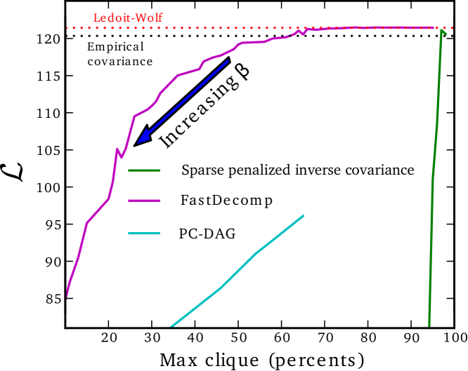
The PC-DAG approach is fast when underlying graphs are very sparse. However, to achieve good cross-validation scores on our data, the p-value on the conditional independence test of the PC algorithm should be very small. As a result, the algorithm explores denser graphs. As the computational cost is in , where is the maximum node degree of the graph, we could not reach an optimal point in reasonable time. We interpret this result by the fact that the brain-connectivity network is poorly represented by a network with small maximum node degree.
5.3 Trading off goodness of fit for decomposition into networks
We are interested in interpreting the graphs in terms of functional networks. As the networks found can be overlapping, the total number of cliques in the decomposable graph is not a good indication of the amount of “decomposition”. For this purpose, we study the maximum clique size, which correspond to the maximum number of nodes in a functional network (Figure 4). With a small maximum clique size, the likelihood of the model (Eq. 4) factors in terms comprising a small amount of brain regions, and the decomposition into conditionally-independent networks in more easily interpretable. Note that, in this case, the description of networks is underpinned by a probabilistic model in which they appear in independent terms, unlike when using ICA [69, 70, 71, 28], or seed-based correlation analysis [30, 72, 1].
Likelihood as a function of clique size
Decomposable models estimated using FastDecomp maintain a generalization score (likelihood on left out data) as good as the baseline for maximum clique size as large as 70% of the number of nodes but for smaller cliques their score decreases, and starts dropping quickly for cliques smaller than 30% (Figure 4). While the models estimated with the sparse penalized inverse covariance estimator or the PC-DAG algorithm are not decomposable, the graph can be completed into a chordal graph151515This procedure is often called triangularization of the graph. using the RCM algorithm. Increasing the penalization to create sparse graphs with the penalized estimator leads to a important loss in generalization scores without a sizable clique width reduction (Figure 4). Indeed, completing the graphs to be chordal creates large cliques unless they are very sparse. This high sparsity is enforced by using a large penalization, which introduces bias in the estimated coefficient and is detrimental to the generalization likelihood. The PC-DAG does not suffer from this limitation. However, we could not use it to explore graphs with a degree higher than 14 due to available computational power as the complexity of this algorithm is exponential in the maximum degree. Although very sparse, these graphs already have large cliques.
Selecting a decomposed model
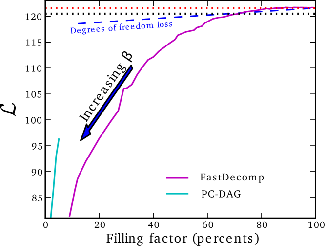
As the maximum clique size decreases, so does the filling factor of the precision matrix. As a result, we are comparing models with different degrees of freedom and we should account for the difference in our model comparison, based on a likelihood ratio test. The expected difference in log-likelihood, under the null hypothesis that two models fit as well the data, is given by half the difference in degrees of freedom. When accounting for this loss (Figure 5), we find that for filling factors above 70%, which corresponds to a maximum clique width of 60%, the model learned by FastDecomp performs as well as the baseline non-sparse model.
5.4 Structure of the models
Here we discuss the structure of brain connectivity that appears in the graph learned.
Very sparse models
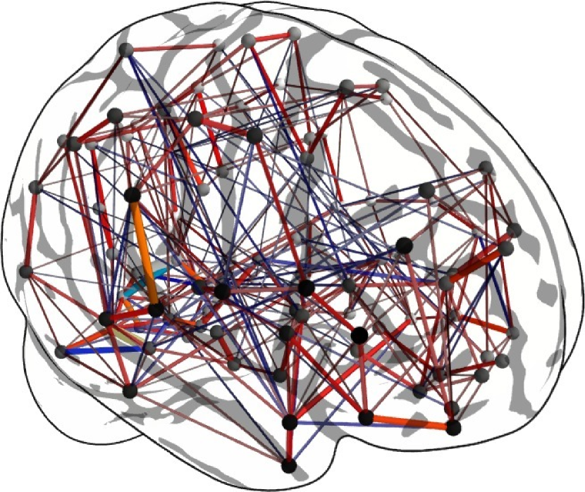
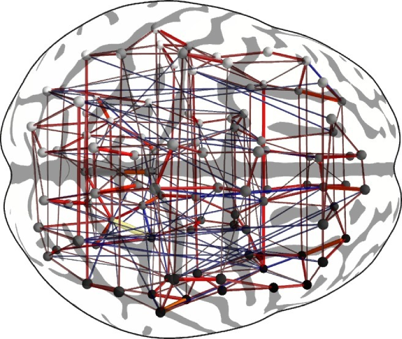
Only very sparse graph structures are directly interpretable. As can be seen on figure 5, PC-DAG is the algorithm best suited for this purpose as, unlike penalized methods, it does not bias the estimation of the precision matrix coefficient, and, unlike the FastDecomp algorithm, it does not force small cliques. It is interesting to note that these graphs have large cliques (Fig 4), even though we were limited to exploring small maximal node degrees161616Strictly speaking, this node degree corresponds to the underlying DAG computed by the PC-DAG algorithm, and not the final undirected graph. due to available computational power. Such graphs (Figure 6) have a lattice-like structure –nearest-neighbor connections on the cortex– with the addition of inter-hemispheric homologous connections and a few long-distance connections.
Decomposition in networks
To assert the meaning of the decomposable models in neuroscientific terms, we apply FastDecomp with chosen such that the maximum clique width is 50% of the full graph. As highlighted by the above cross-validation study, this results in a small loss in generalization scores. However, the resulting cliques and separating sets form small groups of regions and are therefore more interpretable. The estimated banded precision matrix is given in Figure 7. The differences between empirical and estimated covariance accumulate mainly outside the cliques that were selected by FastDecomp, corresponding to the long-range interactions between networks far apart according to the ordering learned. In Figure 8, we display the regions forming the nodes of the graph, colored by their node ordering on a standard brain model.
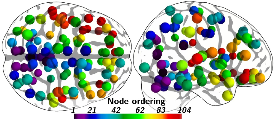
It is clear that the ordering is not random: regions of similar function are grouped together. For instance, the purple nodes form the primary visual cortex and are connected to blue regions along the well-known dorsal visual pathway, going up to the superior parietal lobule [73]. The separation of brain structure from the outer surface versus cingular regions, located in between the hemispheres, is also striking, as well as the symmetry of the model. However, more interesting is that the red regions, representing high node order, form a left-lateral network in the temporal lobe. It resembles the language network, the lateralized network most often recruited that is displayed on figure 1b, as estimated from the same resting-state dataset using an ICA-based method [28]. We note that the ordering of regions located in the central cliques is more difficult to interpret as it appears to be representing several cognitive networks. This is consistent with the fact that these regions are part of larger cliques, that do not separate small structures. We defer a more thorough neuroscientific interpretation of the present results, and in particular a link with the knowledge available from anatomical connectivity data, to future work.
A high bandwidth structure
While the graphical structures that we extract are sparse, we can see that they must have a small average path length to fit the data. Indeed, we find that the adjacency matrix of the graph must have a high bandwidth, as the likelihood drops when forcing a small bandwidth171717The RCM is an algorithm commonly used for ordering a graph to evaluate its bandwidth. as for small clique sizes on figure 4. The graph is therefore a high-bandwidth graph [74], which implies it has a small diameter181818The diameter of a graph is the maximal value of the shortest path lengths for all pairs of nodes in the graph [75]. This in turns implies that average path length on the graph is small. In layman’s term, any two nodes are always connected by a small distance on the graph, as they can not be separated by more than a few large networks.
Small word properties
The high bandwidth that we observed is characteristic of small-world graphs. Our analysis shows that this property is required for a model to fit the data well. The other aspect of a small-world graph, local properties of the graph such as clustering coefficient, is sensitive to sampling noise or the choice of thresholding or any other sparsity-enforcing parameter. It appears that, with our dataset, little sparsity is best to maximize goodness of fit191919The small amount of sparsity may be due to spurious effects, such as inter-subject variability, or the definition of the regions used to extract the signal. We used a standard parcellation of the brain based on the anatomy of a single subject that is used routinely in small world analysis of fMRI – to list only a few [24, 25, 49]– although it has been shown that small-worldness, measured by the ratio of clustering coefficient and average path length, varied as a function of the brain parcellation used [76].. To study the local properties of the graph, we can use the results of the PC-DAG algorithm. Indeed, the chordal completion of the graph used in FastDecomp increases artificially the clustering coefficient, and the penalized estimators give precision matrices that are not sparse enough to be considered as small world202020These precision matrices have many small coefficients, such that thresholding them would put give sparsity level adapted to studying small world properties, however there is no statistically-controlled way of thresholding, as it would also create non positive definite matrices, for which the likelihood of the model is not defined.. On the graph extracted by the PC-DAG with the best goodness of fit, we find an average shortest path length of 3.0 and an average node clustering coefficient of 0.19. These numbers are characteristic of small word graphs [12] and are consistent with the graph properties reported with previous functional-connectivity analysis of fMRI that did not rely on Markov models [26].
We note that the PC-DAG algorithm is ill suited to recover small-world graphs, where the presence of hub nodes leads to high computational costs. On the opposite, FastDecomp is well suited for extracting large interpretable cliques on such data, but not the local properties.
6 Conclusion
We have applied different covariance selection procedures to learn probabilistic graphical models –Markov models– of brain functional connectivity from resting-state fMRI data. We introduce a definition of the large-scale functional networks as the cliques of a decomposable graphical model. To learn efficiently decomposable models on graphs presenting hub nodes, such as small-world graphs, we have introduced a new algorithm. By setting the width of the largest clique of the graph, we have investigated the compromise between models interpretable in terms of independent functional networks, and models that generalize well.
We find that the brain is best represented by a high-bandwidth graph that cannot be decomposed into small cliques: forcing a strongly decomposable representation breaks its small-world properties. However, we can learn a simplified model of the data in which the variables are decomposed into smaller conditionally-independent units that can be interpreted as functional networks, matching the current knowledge in cognitive neuroscience. To summarize adequately brain functional connectivity with segregated networks, these must encompass many brain regions and be strongly overlapping. These preliminary results provide further evidence that the functional connectivity signals observed in fMRI reflect the small-world properties of brain connectivity. Markov models, describing the conditional independence relations of the data, are a promising tool to investigate the large scale architecture of the brain via its functional connectivity.
Acknowledgments
We wish to thank Andreas Kleinschmidt for many enlightening discussions on the cognitive meaning of on-going activity as well as Sepideh Sadiaghiani for acquiring the data used in the paper. We are also grateful to the anonymous reviewers for helpful remarks. This project was partly funded from an INRIA-INSERM collaboration. The fMRI set was acquired in the context of the SPONTACT ANR project (ANR-07-NEURO-042). Estimation algorithms were implemented using the scikit-learn [77]. Figures were generated with Mayavi [78] and nipy (www.nipy.org).
References
References
- Fox and Raichle [2007] M. Fox, M. Raichle, Spontaneous fluctuations in brain activity observed with functional magnetic resonance imaging, Nat Rev Neurosci 8 (2007) 700–711.
- Bullmore and Sporns [2009] E. Bullmore, O. Sporns, Complex brain networks: graph theoretical analysis of structural and functional systems, Nat Rev Neurosci 10 (2009) 186–198.
- Finger [2001] S. Finger, Origins of neuroscience: a history of explorations into brain function, Oxford University Press, USA, 2001.
- Tononi et al. [1998] G. Tononi, G. Edelman, O. Sporns, Complexity and coherency: integrating information in the brain, Trends in cognitive sciences 2 (1998) 474–484.
- Tononi et al. [1994] G. Tononi, O. Sporns, G. Edelman, A measure for brain complexity: relating functional segregation and integration in the nervous system, PNAS 91 (1994) 5033.
- Sporns et al. [2004] O. Sporns, D. Chialvo, M. Kaiser, C. Hilgetag, Organization, development and function of complex brain networks, Trends in Cognitive Sciences 8 (2004) 418–425.
- Varoquaux et al. [2010a] G. Varoquaux, A. Gramfort, J. B. Poline, B. Thirion, Brain covariance selection: better individual functional connectivity models using population prior, in: Advances in Neural Information Processing Systems, 2010a.
- Dehaene et al. [1998] S. Dehaene, M. Kerszberg, J. Changeux, A neuronal model of a global workspace in effortful cognitive tasks, Proceedings of the National Academy of Sciences of the United States of America 95 (1998) 14529.
- Bekinschtein et al. [2009] T. Bekinschtein, S. Dehaene, B. Rohaut, F. Tadel, L. Cohen, L. Naccache, Neural signature of the conscious processing of auditory regularities, Proceedings of the National Academy of Sciences 106 (2009) 1672.
- Fair et al. [2007] D. Fair, N. Dosenbach, J. Church, A. Cohen, S. Brahmbhatt, F. Miezin, D. Barch, M. Raichle, S. Petersen, B. Schlaggar, Development of distinct control networks through segregation and integration, PNAS 104 (2007) 13507.
- Fair et al. [2009] D. Fair, A. Cohen, J. Power, N. Dosenbach, J. Church, F. Miezin, B. Schlaggar, S. Petersen, Functional brain networks develop from a “local to distributed” organization, PLoS Comput Biol 5 (2009) e1000381.
- Watts and Strogatz [1998] D. Watts, S. Strogatz, Collective dynamics of “small-world” networks, Nature 393 (1998) 440–442.
- Strogatz [2001] S. Strogatz, Exploring complex networks, Nature 410 (2001) 268–276.
- Amaral et al. [2000] L. Amaral, A. Scala, M. Barthélémy, H. Stanley, Classes of small-world networks, Proceedings of the National Academy of Sciences of the United States of America 97 (2000) 11149.
- Humphries and Gurney [2008] M. Humphries, K. Gurney, Network “small-world-ness”: a quantitative method for determining canonical network equivalence, PLoS One 3 (2008) e0002051.
- Conturo et al. [1999] T. Conturo, N. Lori, T. Cull, E. Akbudak, A. Snyder, J. Shimony, R. McKinstry, H. Burton, M. Raichle, Tracking neuronal fiber pathways in the living human brain, Proceedings of the National Academy of Sciences of the United States of America 96 (1999) 10422.
- Le Bihan [2003] D. Le Bihan, Looking into the functional architecture of the brain with diffusion MRI, Nature Reviews Neuroscience 4 (2003) 469–480.
- Sporns et al. [2005] O. Sporns, G. Tononi, R. Kotter, The human connectome: a structural description of the human brain, PLoS Comput Biol 1 (2005) e42.
- Hagmann et al. [2008] P. Hagmann, L. Cammoun, X. Gigandet, R. Meuli, C. J. Honey, V. J. Wedeen, O. Sporns, Mapping the Structural Core of Human Cerebral Cortex, PLoS Biol 6 (2008) e159.
- Felleman and Van Essen [1991] D. Felleman, D. Van Essen, Distributed hierarchical processing in the primate cerebral cortex, Cerebral cortex 1 (1) (1991) 1, ISSN 1047-3211.
- Stephan et al. [2001] K. Stephan, L. Kamper, A. Bozkurt, G. Burns, M. Young, R. Kötter, Advanced database methodology for the Collation of Connectivity data on the Macaque brain (CoCoMac), Philosophical Transactions of the Royal Society of London. Series B: Biological Sciences 356 (2001) 1159.
- Sporns et al. [2000] O. Sporns, G. Tononi, G. Edelman, Theoretical neuroanatomy: relating anatomical and functional connectivity in graphs and cortical connection matrices, Cereb Cortex 10 (2000) 127.
- Stam [2004] C. Stam, Functional connectivity patterns of human magnetoencephalographic recordings: a “small-world” network?, Neuroscience letters 355 (2004) 25–28.
- Salvador et al. [2005] R. Salvador, J. Suckling, C. Schwarzbauer, E. Bullmore, Undirected graphs of frequency-dependent functional connectivity in whole brain networks, Philosophical Transactions of the Royal Society B: Biological Sciences 360 (1457) (2005) 937, ISSN 0962-8436.
- Achard et al. [2006] S. Achard, R. Salvador, B. Whitcher, J. Suckling, E. Bullmore, A resilient, low-frequency, small-world human brain functional network with highly connected association cortical hubs, J Neurosci 26 (2006) 63.
- Bassett and Bullmore [2006] D. Bassett, E. Bullmore, Small-world brain networks, The neuroscientist 12 (2006) 512.
- Eguiluz et al. [2005] V. Eguiluz, D. Chialvo, G. Cecchi, M. Baliki, A. Apkarian, Scale-free brain functional networks, Physical review letters 94 (2005) 18102.
- Varoquaux et al. [2010b] G. Varoquaux, S. Sadaghiani, P. Pinel, A. Kleinschmidt, J. Poline, B. Thirion, A group model for stable multi-subject ICA on fMRI datasets, NeuroImage 51 (2010b) 288–299.
- Raichle et al. [2001] M. Raichle, A. MacLeod, A. Snyder, W. Powers, D. Gusnard, G. Shulman, A default mode of brain function, Proceedings of the National Academy of Sciences 98 (2001) 676.
- Biswal et al. [1995] B. Biswal, F. Zerrin Yetkin, V. Haughton, J. Hyde, Functional connectivity in the motor cortex of resting human brain using echo-planar MRI, Magnetic Resonance in Medicine 34.
- Shulman et al. [1997] G. Shulman, J. Fiez, M. Corbetta, R. Buckner, F. Miezin, M. Raichle, S. Petersen, Common blood flow changes across visual tasks: II. Decreases in cerebral cortex, Journal of Cognitive Neuroscience 9 (1997) 648–663.
- Biswal et al. [2010] B. Biswal, M. Mennes, X. Zuo, S. Gohel, C. Kelly, S. Smith, C. Beckmann, J. Adelstein, R. Buckner, S. Colcombe, et al., Toward discovery science of human brain function, Proc Ntl Acad Sci 107 (2010) 4734.
- Damoiseaux et al. [2006] J. S. Damoiseaux, S. A. R. B. Rombouts, F. Barkhof, P. Scheltens, C. J. Stam, S. M. Smith, C. F. Beckmann, Consistent resting-state networks across healthy subjects., Proc Natl Acad Sci U S A 103 (2006) 13848–13853.
- Smith et al. [2009] S. Smith, P. Fox, K. Miller, D. Glahn, P. Fox, C. Mackay, N. Filippini, K. Watkins, R. Toro, A. Laird, et al., Correspondence of the brain’s functional architecture during activation and rest, PNAS 106 (2009) 13040.
- Seeley et al. [2009] W. Seeley, R. Crawford, J. Zhou, B. Miller, M. Greicius, Neurodegenerative Diseases Target Large-Scale Human Brain Networks, Neuron 62 (2009) 42–52.
- Greicius et al. [2009] M. Greicius, K. Supekar, V. Menon, R. Dougherty, Resting-state functional connectivity reflects structural connectivity in the default mode network, Cerebral Cortex 19 (1) (2009) 72, ISSN 1047-3211.
- Van Den Heuvel et al. [2009] M. Van Den Heuvel, R. Mandl, R. Kahn, H. Hulshoff Pol, Functionally linked resting-state networks reflect the underlying structural connectivity architecture of the human brain, Human brain mapping 30 (10) (2009) 3127–3141, ISSN 1097-0193.
- Seeley et al. [2007] W. Seeley, V. Menon, A. Schatzberg, J. Keller, G. Glover, H. Kenna, A. Reiss, M. Greicius, Dissociable intrinsic connectivity networks for salience processing and executive control, The Journal of neuroscience 27 (9) (2007) 2349, ISSN 0270-6474.
- Fox et al. [2005] M. Fox, A. Snyder, J. Vincent, M. Corbetta, D. Van Essen, M. Raichle, The human brain is intrinsically organized into dynamic, anticorrelated functional networks, Proceedings of the National Academy of Sciences of the United States of America 102 (2005) 9673.
- Ioannides [2007] A. Ioannides, Dynamic functional connectivity, Current opinion in neurobiology 17 (2) (2007) 161–170, ISSN 0959-4388.
- Deuker et al. [2009] L. Deuker, E. Bullmore, M. Smith, S. Christensen, P. Nathan, B. Rockstroh, D. Bassett, Reproducibility of graph metrics of human brain functional networks, Neuroimage 47 (4) (2009) 1460–1468, ISSN 1053-8119.
- Bialonski et al. [2010] S. Bialonski, M. Horstmann, K. Lehnertz, From brain to earth and climate systems: Small-world interaction networks or not?, Chaos 20 (2010) 013134.
- Gerhard et al. [2011] F. Gerhard, G. Pipa, B. Lima, S. Neuenschwander, W. Gerstner, Extraction of Network Topology From Multi-Electrode Recordings: Is there a Small-World Effect?, Frontiers in Computational Neuroscience 5.
- Friston [1994] K. Friston, Functional and effective connectivity in Neuroimaging: A synthetis, Hum Brain Map 2 (1994) 56–78.
- Smith et al. [2011] S. Smith, K. Miller, G. Salimi-Khorshidi, M. Webster, C. Beckmann, T. Nichols, J. Ramsey, M. Woolrich, Network modelling methods for FMRI, Neuroimage 54 (2) (2011) 875–891.
- Lauritzen [1996] S. Lauritzen, Graphical models, Oxford University Press, USA, 1996.
- Ledoit and Wolf [2004] O. Ledoit, M. Wolf, A well-conditioned estimator for large-dimensional covariance matrices, J. Multivar. Anal. 88 (2004) 365–411.
- Bickel and Levina [2008] P. Bickel, E. Levina, Regularized estimation of large covariance matrices, The Annals of Statistics 36 (2008) 199–227.
- Huang et al. [2009] S. Huang, J. Li, L. Sun, J. Liu, T. Wu, K. Chen, A. Fleisher, E. Reiman, J. Ye, Learning Brain Connectivity of Alzheimer’s Disease from Neuroimaging Data, in: Advances in Neural Information Processing Systems 22, 808–816, 2009.
- Dempster [1972] A. Dempster, Covariance Selection, Biometrics 28 (1972) 157–175.
- Friedman et al. [2008] J. Friedman, T. Hastie, R. Tibshirani, Sparse inverse covariance estimation with the graphical lasso, Biostatistics 9 (2008) 432–441.
- Banerjee et al. [2006] O. Banerjee, L. Ghaoui, A. d’Aspremont, G. Natsoulis, Convex optimization techniques for fitting sparse Gaussian graphical models, in: ICML, 96, 2006.
- Duchi et al. [2008] J. Duchi, S. Gould, D. Koller, Projected subgradient methods for learning sparse gaussians, in: Proc. of the Conf. on Uncertainty in AI, 2008.
- Spirtes et al. [2001] P. Spirtes, C. Glymour, R. Scheines, Causation, prediction, and search, The MIT Press, 2001.
- Robins et al. [2003] J. Robins, R. Scheines, P. Spirtes, L. Wasserman, Uniform consistency in causal inference, Biometrika 90 (2003) 491.
- Rütimann and Bühlmann [2009] P. Rütimann, P. Bühlmann, High dimensional sparse covariance estimation via directed acyclic graphs, Electron J Stat 3 (2009) 1133–1160.
- Fisher [1915] R. Fisher, Frequency distribution of the values of the correlation coefficient in samples from an indefinitely large population, Biometrika 10 (4) (1915) 507–521.
- Dawid and Lauritzen [1993] A. Dawid, S. Lauritzen, Hyper Markov laws in the statistical analysis of decomposable graphical models, The Annals of Statistics 21 (3) (1993) 1272–1317, ISSN 0090-5364.
- Marrelec et al. [2008] G. Marrelec, P. Bellec, A. Krainik, H. Duffau, M. Pélégrini-Issac, S. Lehéricy, H. Benali, J. Doyon, Regions, systems, and the brain: hierarchical measures of functional integration in fMRI, Medical Image Analysis 12 (2008) 484–496.
- Giudici and Green [1999] P. Giudici, P. Green, Decomposable graphical Gaussian model determination, Biometrika 86 (4) (1999) 785.
- Donnet and Marin [2010] S. Donnet, J. Marin, An empirical Bayes procedure for the selection of Gaussian graphical models, arXiv:1003.5851 .
- Marlin and Murphy [2009] B. Marlin, K. Murphy, Sparse Gaussian graphical models with unknown block structure, in: Proceedings of the 26th International Conference on Machine Learning, ACM, 705–712, 2009.
- Cuthill and McKee [1969] E. Cuthill, J. McKee, Reducing the bandwidth of sparse symmetric matrices, in: Proceedings of the 1969 24th national conference, ACM New York, NY, USA, 157–172, 1969.
- Papadimitriou [1976] C. Papadimitriou, The NP-completeness of the bandwidth minimization problem, Computing 16 (1976) 263–270.
- Chan and George [1980] W. Chan, A. George, A linear time implementation of the reverse Cuthill-McKee algorithm, BIT Numerical Mathematics 20 (1980) 8–14.
- Sadaghiani et al. [2009] S. Sadaghiani, G. Hesselmann, A. Kleinschmidt, Distributed and antagonistic contributions of ongoing activity fluctuations to auditory stimulus detection, Journal of Neuroscience 29 (2009) 13410.
- Tzourio-Mazoyer et al. [2002] N. Tzourio-Mazoyer, B. Landeau, D. Papathanassiou, F. Crivello, O. Etard, N. Delcroix, B. Mazoyer, M. Joliot, Automated anatomical labeling of activations in SPM using a macroscopic anatomical parcellation of the MNI MRI single-subject brain., Neuroimage 15 (2002) 273–289.
- Rothman et al. [2008] A. Rothman, P. Bickel, E. Levina, J. Zhu, Sparse permutation invariant covariance estimation, Electron J Stat 2 (2008) 494.
- Calhoun et al. [2001] V. D. Calhoun, T. Adali, G. D. Pearlson, J. J. Pekar, A method for making group inferences from functional MRI data using independent component analysis., Hum Brain Mapp 14 (2001) 140–151.
- Kiviniemi et al. [2003] V. Kiviniemi, J. Kantola, J. Jauhiainen, A. Hyvärinen, O. Tervonen, Independent component analysis of nondeterministic fMRI signal sources, Neuroimage 19 (2003) 253–260.
- Beckmann et al. [2005] C. F. Beckmann, M. DeLuca, J. T. Devlin, S. M. Smith, Investigations into resting-state connectivity using independent component analysis., Philos Trans R Soc Lond B Biol Sci 360 (2005) 1001–1013.
- Cordes et al. [2000] D. Cordes, V. Haughton, K. Arfanakis, G. Wendt, P. Turski, C. Moritz, M. Quigley, M. Meyerand, Mapping functionally related regions of brain with functional connectivity MR imaging, American Journal of Neuroradiology 21 (2000) 1636–1644.
- Goodale and Milner [1996] M. Goodale, A. Milner, Separate visual pathways for perception and action, Human cognitive neuropsychology: a textbook with readings (1996) 395.
- Gross and Yellen [2004] J. Gross, J. Yellen, Handbook of graph theory, CRC, 2004.
- Chinn et al. [1982] P. Chinn, J. Chvátalová, A. Dewdney, N. Gibbs, The bandwidth problem for graphs and matrices—a survey, Journal of Graph Theory 6 (1982) 223–254.
- Wang et al. [2009] J. Wang, L. Wang, Y. Zang, H. Yang, H. Tang, Q. Gong, Z. Chen, C. Zhu, Y. He, Parcellation-dependent small-world brain functional networks: A resting-state fMRI study, Human brain mapping 30 (2009) 1511–1523.
- Pedregosa et al. [2011] F. Pedregosa, G. Varoquaux, A. Gramfort, V. Michel, B. Thirion, O. Grisel, M. Blondel, P. Prettenhofer, R. Weiss, V. Dubourg, J. Vanderplas, A. Passos, D. Cournapeau, M. Brucher, M. Perrot, D. E., Scikit-learn: Machine Learning in Python, Journal of Machine Learning Research 12 (2011) 2825–2830.
- Ramachandran and Varoquaux [2011] P. Ramachandran, G. Varoquaux, Mayavi: 3D Visualization of Scientific Data, Computing in Science Engineering 13 (2) (2011) 40 –51.