Pattern formation in self-propelled particles with density-dependent motility

Abstract

We study the behaviour of interacting self-propelled particles, whose self-propulsion speed decreases with their local density. By combining direct simulations of the microscopic model with an analysis of the hydrodynamic equations obtained by explicitly coarse graining the model, we show that interactions lead generically to the formation of a host of patterns, including moving clumps, active lanes and asters. This general mechanism could explain many of the patterns seen in recent experiments and simulations.

Collections of self-propelled (SP) particles provide the most common realization of active matter, the study of which constitutes a rapidly growing area of research in physics sriram10 . Examples of SP particles are bacteria, cells Bray and actin filaments “walking” on a carpet of immobilized molecular motors schaller10 .

The term “active” is used to contrast these systems with their passive counterparts, such as solutions of diffusing Brownian particles. Active systems exhibit a much richer physics than their passive counterparts. Most important for us, they have a far larger tendency to form patterns. For instance, bacterial colonies of e.g. E. coli or S. typhimurium growing in the lab can self-organize into crystalline or amorphous arrangements of high-density bacterial clumps murray , while biofilms form even more elaborate patterns such as microbial honeycombs, essentially hexagonal lattices of low-density spots, or voids thar . Similarly, actin in high density motility assays schaller10 organize in moving spots or stripes as well as traveling waves.

What is the mechanism underlying the formation of these “active patterns”? One may expect that, as the underlying constituents of each system are so different, the answer to this question should also be system-specific. If we are to capture all details of a given active pattern, this is indeed likely to be the case. Yet, a fascinating possibility is that there may exist some generic origin of many of these patterns, stemming from a few universal key features of activity, linked to its inherent non-equilibrium nature. In some cases, pursuing such minimal descriptions can be very rewarding. A well-known example is the hydrodynamic theory of flocking proposed by Toner and Tu in toner98 , which was inspired by the “agent-based” model of Vicsek et al. vicsek95 ; sriram10 . The latter studied the dynamics of an ensemble of SP particles subjected to aligning interactions, whose ultimate origin may be hydrodynamic or collision-dominated in the cases of bacteria and actin filaments, or more complex for bird flocks or fish schools. Universal features successfully predicted by generic flocking models are spontaneous motion, giant density fluctuations, and the emergence of complex spatiotemporal active patterns marchetti09 ; marchetti10 .

The original Vicsek model considers point particles of fixed speed and includes no interactions between the SP particles other than a rule that aligns their velocities. Recently, focus has shifted onto specific models where additional interactions are included, most commonly steric repulsion gregoire2003 ; peruani06 ; baskaran08 ; yang10 ; marchetti11 ; peruani11 ; notestericrepulsion . Our aim here is to develop a more generic model for interacting SP particles. Interactions are incorporated in our model by assuming that the motility of the SP particles is a decreasing function of their local density note1 . One may envisage several physical mechanisms responsible for a decay of the propulsion velocity with density: here we highlight just two. First, such a slowdown may arise due to local crowding and steric hindrance, just as in peruani06 ; baskaran08 ; peruani11 ; marchetti11 . An alternative mechanism can be provided by biochemical signaling such as quorum sensing in bacterial colonies, as recently explored theoretically cates10 and experimentally Hwa11 . This second mechanism may lead to slowdown even in dilute suspensions. Our work describes the results of simulations of a microscopic SP particles model with both interactions and alignment rule, the derivation of the corresponding hydrodynamic description of the model in terms of a density and a polarization field, and an analysis of the continuum theory. It therefore provides a direct bridge between microscopic and continuum models, which allows us to identify universal mechanisms driving pattern formation in interacting SP particles. As we shall see, interactions lead to an even larger repertoire of patterns in active particle suspensions than obtained in conventional Vicsek models. These include moving clumps, lanes and asters, and qualitatively match the patterns found experimentally, e.g. in schaller10 . Our hydrodynamic equations also provide an understanding of the origin of the various patterns and allow us a clear comparison with other interacting active particle models.

We consider a modified version of the Vicsek model vicsek95 , where the particles interact via a pairwise aligning forcing, which simplifies the coarse graining of the microscopic model. In 2D the position $r_{i}$ and direction, identified by an angle $\theta_{i}$ (or a vector $\mathbf{e}_{\theta_{i}}$), of the $i$th particle evolve according to

$${\dot{r}_{i}=v\,\mathbf{e}_{\theta_{i}};\>\dot{\theta}_{i}=\gamma\sum_{j}F(\theta_{j}-\theta_{i},r_{j}-r_{i})+\sqrt{2\epsilon}\tilde{\eta}_{i}(t)}$$ (1)

where $\gamma$ and $\epsilon$ are parameters describing the strength of alignment and fluctuations respectively, and $\tilde{\eta}(t)$ is a Gaussian white noise with zero mean and unit variance. $F$ controls the alignment interactions between the spins. For simplicity, we choose $F(\theta,r)=\sin(\theta)/\pi R^{2}$ if $|r|<R$ and $0$ otherwise, though its precise shape does not dramatically affect the physics. In the $v\to 0$ limit, our model is an off-lattice analogue of the XY model for a ferromagnet, hence we call it the flying XY model. This differs from other models of SP particles where alignment is explicitly due to ‘collisions’, and in which the interaction strength vanishes as $v\to 0$ bertin09 . Such cases can however be recovered by taking $\gamma\propto v$. Last, a density-dependent velocity is introduced in the model by stipulating that $v$ depends on the number of particles $n$ within a given radius $R_{n}$, as $v(n)=v_{0}e^{-\lambda n}+v_{1}$, where $v_{0}\gg v_{1}>0$ are the dilute and crowded limiting velocities respectively, and $\lambda>0$ controls the decay of the motility decreases with increasing density. Hereupon we restrict to $R_{n}=R$.

Fig. 1A shows a representative phase diagram of the flying XY model in the $(\epsilon,\lambda)$ plane. For small $\lambda$, when $v$ is practically constant, the phases observed are the same as those in the literature on flocking models vicsek95 ; chate04 . Namely, at high $\epsilon$ we find a disordered, homogeneous state (region c in Fig. 1A), followed by a polarly ordered phase with high density stripes (named stripy phase, b in Fig. 1A) below a critical noise value. For even lower $\epsilon$, we observe a ‘fluctuating flocking state’ (region a) with polar order and large density fluctuations – this state is very close to the one described in Ref. marchetti10 and we do not discuss it further here. These phases are expected – as we shall see below the hydrodynamic equations for our model map to those for the Vicsek model toner98 ; marchetti10 when $v$ is constant.

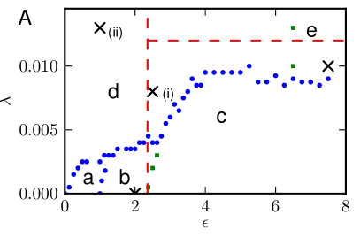
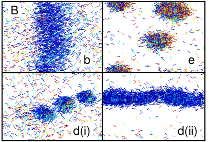
Figure 1: (color online) (A) Phase diagram in the $(\epsilon,\lambda)$ plane, for $N=3000$, $L=10$, $\gamma=0.16$, $v_{0}=2$ and $v_{1}=0.1$. Blue filled circles on the phase boundary correspond to peaks in the variance of the particle density, while green squares separate states with zero mean orientation from states with nonzero mean orientation. Phases are labelled as per discussion in the text. Horizontal and vertical red lines indicate linear instabilities towards clustering and ordering, respectively. (B) Snapshots of the stripy (b), aster (e), moving clumps (d(i)), lane (d(ii)) patterns. The crosses in A correspond to the snapshots in B. Particles are color coded by direction, with blue horizontal and red vertical.

Above a critical value $\lambda_{c}(\epsilon)$, new patterns appear. Due to the density-dependent motility, the SP particles cluster via a self-trapping mechanism through which they assemble and slow-down, creating a positive feedback loop akin to the one discussed for models of bacteria cates10 . This process leads to the formation of high density clumps which slowly coarsen towards a fully phase separated steady state. The Vicsek-like alignment tendency greatly affects this instability. On one hand, the critical value $\lambda_{c}(\epsilon)$ decreases almost to zero with decreasing $\epsilon$. Furthermore, the presence of polar order promoted by the alignment changes the nature of the clusters. In Fig. 1A we identify at least three distinct patterns, of which snapshots are shown in Fig. 1B. When $\epsilon$ is small, rather than structureless dots, the clusters show an orientational order and move coherently: they form “moving clumps” (pattern d(i) in Fig. 1). For low $\epsilon$ and large $\lambda$ the moving clumps merge into bands, or lanes (labelled as d(ii)) – within these, however, particles move parallel rather than perpendicular to the band, in contrast with the $\lambda\to 0$ stripy phase. This is reminiscent of the ‘streaks’ of actin filaments observed in schaller10 . In the disordered, high $\epsilon$ phase, the clusters instead diffuse randomly, and are on average stationary.

Here, a temporal average of the particle orientation patterns shows that the clusters are asters (the aster phase is labelled as e in Fig. 1). However, as discussed in greater detail below, the orientation in the aster is non-standard: particles point towards its center at the core, but they coherently point outwards in its periphery. We stress that moving clusters, lanes and asters are not observed either in the standard Vicsek model, or in its standard mean field continuum description used in Ref. marchetti10 . They are a consequence of the interplay between self-propulsion, alignment and density-dependent motility: switching off any of these ingredients would thus greatly reduce the pattern forming potential of the model.

To get a better understanding of the pattern formation process, we now discuss how to coarse grain the microscopic dynamics (1) to obtain a macroscopic description of the model. They are two candidates for the hydrodynamic fields: the particle density $\rho$, which is conserved, and the local alignment, or polarization, vector ${\mathbf{P}}$, on symmetry ground. Note that “hydrodynamic” here means slowly varying in space and time – the dynamics of the underlying fluid is not included in our modeling. Following Ref. dean96 , we start with the microscopic Eq. (1) and use Itō calculus cates10 to write down a stochastic dynamical equation for the evolution of $f(\mathbf{r},\theta,t)$, the density of particles at position $\mathbf{r}$ with angle $\theta$, as follows

$$\partial_{t}f(\mathbf{r},\theta)+\mathbf{e}_{\theta}\cdot\nabla[vf]=\epsilon\frac{\partial^{2}f}{\partial\theta^{2}}-\frac{\partial}{\partial\theta}\sqrt{2\epsilon f}\eta$$ (2)

$$-\gamma\frac{\partial}{\partial\theta}\int d\theta^{\prime}d{\mathbf{r}^{\prime}}f(\mathbf{r^{\prime}},\theta^{\prime})f(\mathbf{r},\theta)F(\theta^{\prime}-\theta,\mathbf{r}-\mathbf{r^{\prime}}).$$

The second term on the left hand side describes familiar advection, but with one important difference: the velocity $v$ appears inside the gradient. This is precisely what leads to the instabilities responsible for the new patterns in the simulations. By dropping the conserved noise $\sqrt{2\epsilon f}\eta$, we obtain a non-fluctuating kinetic equations for the flying XY model. Following Bertin et al. bertin09 , we Fourier transforms Eq. 2 to get equations of motion for $f_{k}\equiv\int fe^{ik\theta}d\theta$. Using $2\pi f(\theta)=\sum_{k}f_{k}e^{-ik\theta}$ and $2\pi F(\theta)=\sum_{k}F_{k}e^{-ik\theta}$, we obtain a hierarchy of equations:

$$\partial_{t}f_{k}+\frac{\partial}{\partial x}\frac{vf_{k+1}+vf_{k-1}}{2}+\frac{\partial}{\partial y}\frac{vf_{k+1}-vf_{k-1}}{2i}$$ (3)

$$=-k^{2}\epsilon f_{k}+i\frac{\gamma k}{2\pi}\sum_{m}f_{m}F_{-m}f_{k-m},$$

where all sums run from $-\infty$ to $+\infty$. In principle, $F$ is slightly non-local in space so that the second term of the r.h.s. of Eq. (3) should retain a spatial integral. We are however interested in the hydrodynamic, large-scale, description of the system, a limit in which $R$ is very small and we assume $F$ to be perfectly local note2 . To obtain mean field equations for the hydrodynamic variables, we note that $f_{k}$ for $k=0$ is simply the density, $\rho$, whereas the real and imaginary part of $f_{1}$ are the $x$ and $y$ component of $\rho\mathbf{P}$ respectively (as we work in 2D we can identify vectors with complex numbers). By writing out in full the $k=0$ case of Eq. (2), we then find that the density field obeys the continuity equation

$$\partial_{t}\rho=-\nabla\cdot(v\mathbf{W}),$$ (4)

where ${\mathbf{W}}\equiv\rho{\mathbf{P}}$. To make further progress, we now assume that we are not too deeply in the ordered phase, so that $f(\theta)$ is to first order approximation homogeneous, hence higher Fourier components ($f_{k}$ for $k\geq 3$) may be neglected. Following bertin09 , we further assume that $f_{2}$ is a fast variable, so that $\dot{f_{2}}\simeq 0$. After lengthy but straightforward algebra, we obtain the following equation for ${\mathbf{W}}$,

$$\partial_{t}\mathbf{W}+\frac{\gamma}{16\epsilon}(\mathbf{W}\cdot\nabla)(v\mathbf{W})=(\frac{1}{2}\gamma\rho-\epsilon)\mathbf{W}$$ (5)

$$-\frac{\gamma^{2}}{8\epsilon}W^{2}\mathbf{W}-\frac{1}{2}\nabla(v\rho)+\frac{3\gamma}{16\epsilon}\nabla(vW^{2})$$

$$-\frac{\gamma}{32\epsilon}v\nabla W^{2}-\frac{3\gamma}{16\epsilon}\mathbf{W}\nabla\cdot(v\mathbf{W})$$

$$-\frac{\gamma}{8\epsilon}v\mathbf{W}(\nabla\cdot\mathbf{W})-\frac{\gamma}{8\epsilon}v(\mathbf{W}\cdot\nabla)\mathbf{W}+{\cal O}(\nabla^{2})$$

The second term on the l.h.s. of Eq. (5) describes self-advection of particles and breaks Galilean invariance toner98 . The first two terms on the right-hand side describe the standard spontaneous symmetry breaking leading to polar order and flocking for sufficiently small $\epsilon$ in the Vicsek model at $\lambda=0$. The third, pressure-like term, $-\frac{1}{2}\nabla(v\rho)$, is the most relevant one in our work, as it is responsible for the clustering instability observed in Fig. 1 when $\lambda\neq 0$. Higher order terms in $\nabla$ and $\mathbf{W}$ have minor effects on patterns and will be discussed elsewhere.

Having written down the mean field equations of motion, Eqs. (4) and (5), we can now assess how their predictions compare with the full simulations of the microscopic model. The continuum theory predicts an order-disorder transition at $\epsilon_{c}=\frac{1}{2}\gamma\rho_{0}$. For $\epsilon>\epsilon_{c}$ there is a stable homogeneous disordered state, with $\rho=\rho_{0}$ and $\mathbf{W}=0$. For $\epsilon<\epsilon_{c}$ the equations yield a homogeneous ordered or flocking state with $\rho=\rho_{0}$ and $\mathbf{W}=W_{0}{\bf\hat{x}}$, where we have chosen the $x$ axis along the direction of broken symmetry and $W_{0}=\sqrt{8\epsilon(\epsilon_{c}-\epsilon)/\gamma^{2}}$. The mean-field transition at $\epsilon_{c}$ does not depend on $\lambda$ and coincides with that of the equilibrium XY model. The order-disorder phase boundary predicted by the theory is compared to its numerical counterpart in Fig. 2A. We then study the linear stability of the homogeneous disordered state at $\epsilon>\epsilon_{c}$ against spatially inhomogeneous fluctuations. It is straightforward to show that when $\lambda\neq 0$ the homogeneous disordered phase becomes unstable for all wavenumbers when $v(\rho_{0})+\rho_{0}v^{\prime}(\rho_{0})<0$. This instability, referred to as a clustering instability, arises due to the term - $\frac{1}{2}\nabla(v\rho)$ in the equation for $\mathbf{W}$. The threshold between homogeneous and clustered phases found numerically at large $\epsilon$ is close to but below the prediction (Fig. 2B). This is reasonable, as the linear stability can only access the spinodal line: fluctuations may trigger phase separation for lower $\lambda$.

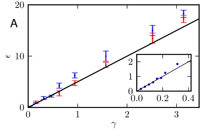
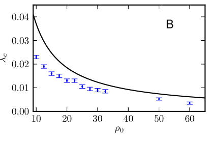
Figure 2: (color online) (A) Phase boundary for the flying XY model when $\lambda=0$, showing the critical value of $\epsilon$ as a function of $\gamma$. Blue points for $v=2.0$, red for $v=0.5$. Inset: data for $v=2.0$ for smaller values of $\gamma$, showing good agreement. (B) Phase boundary for $\epsilon=5$, $\gamma=0.16$. In all cases $L=10$ and $N=1000$.

To go beyond the simple linear stability analysis of the homogeneous disordered state, account for the effect of the non-linear terms, and hence explore the range of patterns compatible with our hydrodynamics equations, we solved Eqs. (4) and (5) numerically, by means of a standard finite difference scheme. In order to enhance the stability of our algorithm, we included a diffusive term $D\nabla^{2}\rho$ on the right hand side of Eq. (4). Our numerical results show that all the five patterns, or phases, observed in the microscopic simulations (fluctuating flocking state, moving stripes and lanes, static asters and moving clumps) can be found within Eqs. (4) and (5) – Fig. 3 portrays a comparison of the $\lambda\neq 0$ patterns. Interestingly the origin of the atypical asters can be directly read in Eq. (5). In the steady-state, low gradient, small ${\mathbf{W}}$ approximation, Eq. (5) reduces to $(\gamma\rho/2-\epsilon)\mathbf{W}=\nabla(\rho v/2)$ and $\nabla(v\rho)$ thus acts as an ordering field for ${\mathbf{W}}$. Along the radius of an aster, the density increases towards the center whereas the velocity decreases. Their product can thus be non-monotonous, which makes $\mathbf{W}$ change direction, whence the atypical asters seen in the microscopic simulations. In the continuum simulations, even though $\nabla\rho v$ can change sign, the presence of the diffusive terms disallows sharp gradients and we did not find parameters for which $\nabla\rho v$ was dominating. We could, however, end up with both inward pointing or outward pointing asters, corresponding to phases with high-density clumps (at small $\lambda$, shown in Fig. 3C) or low-density voids (at larger $\lambda$, similar to those discussed in thar , not shown).

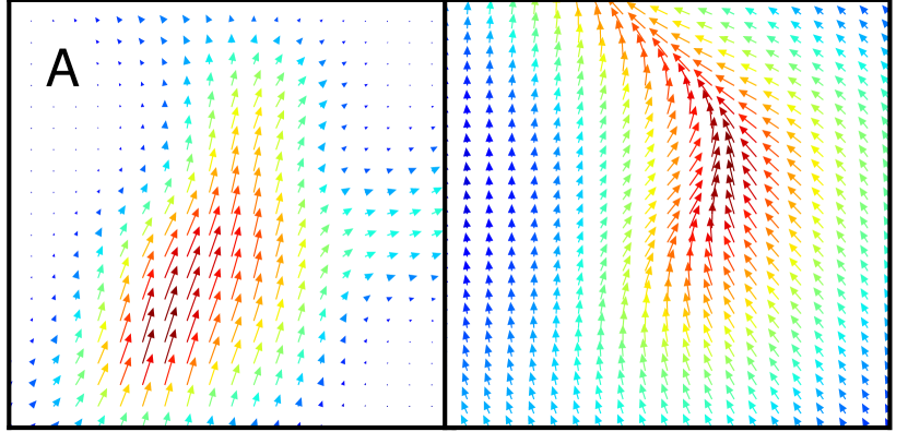
$\tilde{\lambda}$	0.75	1.5
$\tilde{v_{1}}$	0.05	0.09
$\tilde{\gamma}$	1.6	3.6
$\tilde{D}$	-	0.02

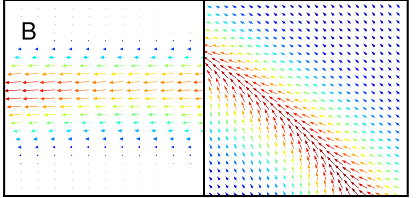
$\tilde{\lambda}$	1.2	1.5
$\tilde{v_{1}}$	0.05	0.12
$\tilde{\gamma}$	4.8	4.5
$\tilde{D}$	-	0.02

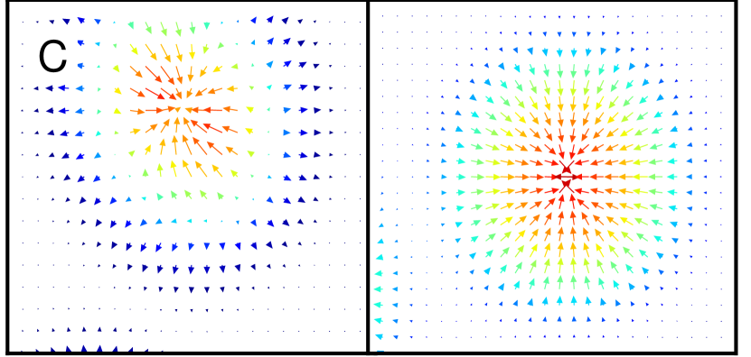
$\tilde{\lambda}$	0.94	1.5
$\tilde{v_{1}}$	0	0
$\tilde{\gamma}$	0.64	2.3
$\tilde{D}$	-	0.01

Figure 3: (color online) Patterns found for $\lambda\neq 0$ in the microscopic simulations (left column) and in the numerical solution of the hydrodynamic equations (right). Tables show dimensionless parameter values: $\tilde{\lambda}=\lambda\rho_{0}$, $\tilde{v_{1}}=v_{1}/v_{0}$, $\tilde{\gamma}=\gamma\rho_{0}/\epsilon$, $\tilde{D}=D\epsilon/v_{0}^{2}$. Arrows show the ${\mathbf{W}}$ field, colors the density (red: high; blue: low).

We have shown that a density-dependent motility in our flying XY model, which is a close relative of the Vicsek model, yields new patterns in suspensions of SP particles. Such patterns include moving clumps, lanes, and asters, associated with high-density clumps, or voids. All these patterns have experimental counterparts schaller10 ; murray ; thar . By explicitly linking the microscopic and coarse grained mean field dynamics, we were able to identify the key ingredients which trigger the appearance of the new patterns in the “pressure term” $-\frac{1}{2}\nabla(v\rho)$: when this turns negative, new patterns may form. Importantly, the patterns we see are not very sensitive to the precise form of $v(\rho)$. For instance, steric hindrance results in velocities that typically decrease linearly with density thompson2011 and would give similar instabilities.

We close with a comparison with other models featuring patterns similar to ours. Continuum models for microtubule-kinesin solutions leading to aster formation have been proposed in leekardar . The resulting equations of motion for the microtubule polarisation included a phenomenological term of the form $S\nabla(\rho)$ with $S>0$, and $\rho$ the density of motors bound to microtubules. This is qualitatively similar to our equations with negative $-\frac{1}{2}\nabla(v\rho)$. In the $\lambda=0$ limit, Refs. bertin09 ; marchetti10 show that asters are absent if the prefactors in the non-linear terms in the continuum equations are obtained via a systematic coarse-graining of a system of Vicsek SP particles or SP hard rods. Ref. gopinath shows, however, that asters do appear if these prefactors are tuned as independent parameters, although in this case the asters have fixed polarity.

Finally, Peruani et al. peruani11 studied a microscopic lattice variant of the Vicsek model, and also found asters and moving clumps, dubbed traffic jams and gliders respectively. The underlying passive model in Ref. peruani11 is the 4-state Potts model, which is in a different universality class than the XY model, to which our dynamics reduces in the passive limit. However, the active patterns are similar in the two models. This is again naturally explained by our theory, as their origin in peruani11 lies in the slowdown of particles due to crowding jamming, which brings up an effective “pressure term” analogous to the one in Eq. (5). A density-dependent motility, induced either by steric hindrance or by crosslinkers between actin filaments, may also at the basis of the formation of similar patterns in the actin-walker experiments in schaller10 .

We thank M. R. Evans for useful discussions. MCM was supported by the National Science Foundation through awards DMR-0806511 and DMR-1004789.

References

- (1) S. Ramaswamy, J. F. Joanny, Nature 467, 33 (2010); S. Ramaswamy, Annu. Rev. Cond. Matt. Phys. 1, 323 (2010).
- (2) D. Bray, Cell Movements: From Molecules to Motility, 2nd Edition, Garland Publishing, New York (2001).
- (3) V. Schaller et al., Nature 467, 73 (2010); S. Köhler et al., Nat. Mat. 10, 462 (2011), V. Schaller et al., Proc. Natl. Acad. Sci. USA., early-edition (2011).
- (4) J. D. Murray, Mathematical Biology, Vol. 2, Springer-Verlag, Berlin (2003).
- (5) R. Thar, M. Kuhl, FEMS Microbiol. Lett. 246, 75 (2005).
- (6) J. Toner and Y. H. Tu, Phys. Rev. Lett. 75, 4326 (1995); Phys. Rev. E 58, 4828 (1998); J. Toner et al., Ann. Phys. 318, 170 (2005).
- (7) T. Vicsek et al. Phys. Rev. Lett. 75, 1226 (1995).
- (8) A. Baskaran and M. C. Marchetti, Proc. Natl. Acad. Sci. USA 106, 15567 (2009).
- (9) S. Mishra et al.Phys. Rev. E 81, 061916 (2010).
- (10) G. Gregoire, H. Chaté and Y. Tu, Physica D 181, 187 (2003).
- (11) F. Peruani, A. Deutsch, and M. Bär, Phys. Rev. E 74, 030904(R) (2006).
- (12) A. Baskaran and M. C. Marchetti, Phys. Rev. Lett. 101, 268101 (2008).
- (13) Y. Yang, V.Marceau and G. Gompper, Phys. Rev. E 82, 031904 (2010).
- (14) S. Henkes et al.,Phys. Rev. E 84, 040301(R) (2011); S. R. McCandlish et al., arXiv:1110.2479.
- (15) F. Peruani et al., Phys. Rev. Lett. 106, 128101 (2011); F. Ginelli et al., Phys. Rev. Lett. 104, 184502 (2010).
- (16) One should further distinguish between collection of sterically interacting SP particles where alignment is imposed a-la-Vicsek, and others were it comes solely from steric repulsion of rod-like particles peruani06 ; baskaran08 ; yang10 ; peruani11 . In the latter case steric repulsion aligns SP particles regardless of their polarity, yielding nematic rather than polar order.
- (17) Other functional dependencies lead to a less rich physics – details will be given elsewhere.
- (18) J. Tailleur and M. E. Cates, Phys. Rev. Lett. 100, 218103 (2008); M. E. Cates et al., Proc. Natl. Acad. Sci. USA 107, 11715 (2010);
- (19) C. Liu et al, Science 334, 238 (2011).
- (20) E. Bertin, M. Droz and G. Gregoire. J. Phys. A 42, 445001 (2009).
- (21) G. Gregoire and H. Chaté, Phys. Rev. Lett. 92, 025702 (2004).
- (22) D. S. Dean, J. Phys. A: Math. Gen. 29 L613 (1996).
- (23) A non-local can be dealt e.g. as in cates10 .
- (24) A. G. Thompson et al., J. Stat. Mech. P02029 (2011).
- (25) H. Y. Lee and M. Kardar, Phys. Rev. E 64, 056113 (2001); S. Sankararaman et al.,Phys. Rev. E 70, 031905 (2004).
- (26) A. Gopinath et al., arXiv:1112.6011; K. Gowrishankar and M. Rao, arXiv:1201.3938.