Long runs under a conditional limit distribution

Abstract

This paper presents a sharp approximation of the density of long runs of a random walk conditioned on its end value or by an average of a function of its summands as their number tends to infinity. In the large deviation range of the conditioning event it extends the Gibbs conditional principle in the sense that it provides a description of the distribution of the random walk on long subsequences. An approximation of the density of the runs is also obtained when the conditioning event states that the end value of the random walk belongs to a thin or a thick set with a nonempty interior. The approximations hold either in probability under the conditional distribution of the random walk, or in total variation norm between measures. An application of the approximation scheme to the evaluation of rare event probabilities through importance sampling is provided. When the conditioning event is in the range of the central limit theorem, it provides a tool for statistical inference in the sense that it produces an effective way to implement the Rao–Blackwell theorem for the improvement of estimators; it also leads to conditional inference procedures in models with nuisance parameters. An algorithm for the simulation of such long runs is presented, together with an algorithm determining the maximal length for which the approximation is valid up to a prescribed accuracy.

and

1 Context and scope.

This paper explores the asymptotic distribution of a random walk conditioned on its final value as the number of summands increases. Denote $\mathbf{X}_{1}^{n}:=(\mathbf{X}_{1},\ldots,\mathbf{X}_{n})$ a set of $n$ independent copies of a real random variable $\mathbf{X}$ with density $p_{\mathbf{X}}$ on $\mathbb{R}$ and $\mathbf{S}_{1,n}:=\mathbf{X}_{1}+\cdots+\mathbf{X}_{n}$. We consider approximations of the density of the vector $\mathbf{X}_{1}^{k}=(\mathbf{X}_{1},\ldots,\mathbf{X}_{k})$ on $\mathbb{R}^{k}$ when $\mathbf{S}_{1,n}=na_{n}$, and $a_{n}$ is a convergent sequence. The integer valued sequence $k:=k_{n}$ is such that

$$0\leq\lim\sup_{n\rightarrow\infty}k/n\leq{1}$$ (K1)

together with

$$\lim_{n\rightarrow\infty}n-k=\infty.$$ (K2)

Therefore we may consider the asymptotic behavior of the density of the trajectory of the random walk on long runs. For the sake of applications we also address the case when $\mathbf{S}_{1,n}$ is substituted by $\mathbf{U}_{1,n}:=u(\mathbf{X}_{1})+\cdots+u(\mathbf{X}_{1})$ for some real valued measurable function $u$, and when the conditioning event is $(\mathbf{U}_{1,n}=u_{1,n})$ where $u_{1,n}/n$ converges as $n$ tends to infinity. A complementary result provides an estimation for the case when the conditioning event is a large set in the large deviation range, $(\mathbf{U}_{1,n}\in nA)$ where $A$ is a Borel set with nonempty interior with $Eu(\mathbf{X})<\mathtt{essinf}A$; two cases are considered, according to the local dimension of $A$ at its essential infimum point essinf$A$.

The interest in this question stems from various sources. When $k$ is fixed (typically $k=1$) this is a version of the Gibbs conditional principle which has been studied extensively for fixed $a_{n}\neq E\mathbf{X}$, therefore under a large deviation condition. Diaconis and Freedman DiaconisFreedman1988 have considered this issue also in the case $k/n\rightarrow\theta$ for $0\leq\theta<1$, in connection with de Finetti’s theorem for exchangeable finite sequences. Their interest was related to the approximation of the density of $\mathbf{X}_{1}^{k}$ by the product density of the summands $\mathbf{X}_{i}$’s, and therefore on the validity of the independence of the $\mathbf{X}_{i}$’s under conditioning. Their result is in the spirit of Van Camperhout and Cover VanCamperhoutCover1981 , and parallels can be drawn with Csiszár’s Csiszar1084 asymptotic conditional independence result, when the conditioning event is $(\mathbf{S}_{1,n}>na_{n})$ with $a_{n}$ fixed and larger than $E\mathbf{X}$. In the same vein and under the same large deviation condition Dembo and Zeitouni DemboZeitouni1996 considered similar problems. This question is also of importance in statistical physics. Numerous papers pertaining to structural properties of polymers deal with this issue, and we refer to denHollanderWeiss1988 and denHollanderWeiss1988a for a description of those problems and related results. In the moderate deviation case, Ermakov ERmakov2006 also considered a similar problem when $k=1$.

The approximation of conditional densities is the basic ingredient for the numerical estimation of integrals through improved Monte Carlo techniques. Rare event probabilities may be evaluated through importance sampling techniques; efficient sampling schemes consist of the simulation of random variables under a proxy of a conditional density, often with respect to conditioning events of the form $(\mathbf{U}_{1,n}>na_{n})$; optimizing these schemes has been a motivation for this work.

In parametric statistical inference, conditioning on the observed value of a statistic leads to a reduction of the mean square error of some estimate of the parameter; the famous Rao–Blackwell and Lehmann–Scheffé theorems can be implemented when a simulation technique produces samples according to the distribution of the data conditioned on the value of some observed statistics. In these applications the conditioning event is local, and when the statistic is of the form $\mathbf{U}_{1,n}$, then the observed value $u_{1,n}$ satisfies $\lim_{n\rightarrow\infty}u_{1,n}/n=Eu(\mathbf{X})$. Such is the case in exponential families when $\mathbf{U}_{1,n}$ is a sufficient statistic for the parameter. Other fields of applications pertain to parametric estimation where conditioning by the observed value of a sufficient statistic for a nuisance parameter produces optimal inference via maximum likelihood in the conditioned model. In general this conditional density is unknown; the approximation produced in this paper provides a tool for the solution of these problems.

For both importance sampling and for the improvement of estimators, the approximation of the conditional density of $\mathbf{X}_{1}^{k}$ on long runs should be of a special form: it has to be a density on $\mathbb{R}^{k}$, easy to simulate, and the approximation should be sharp. For these applications the relative error of the approximation should be small on the simulated paths only. Also for inference via maximum likelihood under nuisance parameters the approximation has to be accurate on the sample itself and not on the entire space.

Our first set of results provides a very sharp approximation scheme; numerical evidence on exponential runs with length $n=1000$ provide a relative error of the approximation of order less than 100% for the density of the first 800 terms when evaluated on the sample paths themselves, thus on the significant part of the support of the conditional density; this very sharp approximation rate is surprising in such a large dimensional space, and it illustrates the fact that the conditioned measure occupies a very small part of the entire space. Therefore the approximation of the density of $\mathbf{X}_{1}^{k}$ is not performed on the sequence of entire spaces $\mathbb{R}^{k}$, but merely on a sequence of subsets of $\mathbb{R}^{k}$ which contain the trajectories of the conditioned random walk with probability going to $1$ as $n$ tends to infinity; the approximation is performed on typical paths.

The extension of our results from typical paths to the whole space $\mathbb{R}^{k}$ holds: convergence of the relative error on large sets imply that the total variation distance between the conditioned measure and its approximation goes to $0$ on the entire space. So our results provide an extension of Diaconis and Freedman DiaconisFreedman1988 and Dembo and Zeitouni DemboZeitouni1996 who considered the case when $k$ is of small order with respect to $n$; the conditions which are assumed in the present paper are weaker than those assumed in the previously cited works; however, in contrast with their results, we do not provide explicit rates for the convergence to $0$ of the total variation distance on $\mathbb{R}^{k}$.

It would have been of interest to consider sharper convergence criteria than the total variation distance; the $\chi^{2}$-distance, which is the mean square relative error, cannot be bounded through our approach on the entire space $\mathbb{R}^{k}$, since it is only suitable for large sets of trajectories (whose probability goes to $1$ as $n$ increases); this is not sufficient to bound its expected value under the conditional sampling.

This paper is organized as follows. Section 2 presents the approximation scheme for the conditional density of $\mathbf{X}_{1}^{k}$ under the conditioning point sequence $(\mathbf{S}_{1,n}=na_{n})$. In Section 3, it is extended to the case when the conditioning family of events is written as $(\mathbf{U}_{1,n}=u_{1,n})$. The value of $k$ for which this approximation is appropriate is discussed; an algorithm for the implementation of this rule is proposed. Algorithms for the simulation of random variables under the approximating scheme are also presented. Section 4 extends the results of Section 3 when conditioning on large sets. Two applications are presented in Section 5; the first one pertains to Rao–Blackwellization of estimators, hence on the application of the results of Section 3 when the conditioning point is such that $\lim_{n\rightarrow\infty}u_{1,n}/n=Eu(\mathbf{X})$; in the second application the result of Section 4 is used to derive small variance estimators of rare event probabilities through importance sampling; in this case the conditioning event is in the range of the large deviation scale.

The main steps of the proofs are in the core of the paper; some of the technicalities are left to the Appendix.

2 Random walks conditioned on their sum.

2.1 Notation and hypothesis.

In this section the conditioning point event is written as

$$\mathcal{E}_{n}:=(\mathbf{S}_{1,n}=na_{n}).$$

We assume that $\mathbf{X}$ satisfies the Cramér condition; that is, $\mathbf{X}$ has a finite moment generating function $\Phi(t):=E[\exp(t\mathbf{X})]$ in a nonempty neighborhood of $0$. Denote

$$m(t) := \frac{d}{dt}\log\Phi(t),$$

$$s^{2}(t) := \frac{d}{dt}m(t),$$

$$\mu_{3}(t) := \frac{d}{dt}s^{2}(t).$$

The values of $m(t)$, $s^{2}$ and $\mu_{3}(t)$ are the expectation, the variance and the kurtosis of the tilted density

$$\pi^{\alpha}(x):=\frac{\exp(tx)}{\Phi(t)}p(x),$$ (1)

where $t$ is the unique solution of the equation $m(t)=\alpha$ when $\alpha$ belongs to the support of $\mathbf{X}$. Conditions on $\Phi(t)$ which ensure existence and uniqueness of $t$ are referred to as steepness properties; we refer to Barndorff1978 , page 153 ff., for all properties of moment generating functions used in this paper. Denote $\Pi^{\alpha}$ the probability measure with density $\pi^{\alpha}$.

We also assume that the characteristic function of $\mathbf{X}$ is in $L^{r}$ for some $r\geq 1$ which is necessary for the Edgeworth expansions to be performed.

The probability measure of the random vector $\mathbf{X}_{1}^{n}$ on $\mathbb{R}^{n}$ conditioned upon $\mathcal{E}_{n}$ is denoted $P_{na_{n}}$. We also denote $P_{na_{n}}$ the corresponding distribution of $\mathbf{X}_{1}^{k}$ conditioned upon $\mathcal{E}_{n}$; the vector $\mathbf{X}_{1}^{k}$ then has a density with respect to the Lebesgue measure on $\mathbb{R}^{k}$ for $1\leq k<n$, which will be denoted $p_{na_{n}}$. For a general r.v. $\mathbf{Z}$ with density $p$, $p(\mathbf{Z}=z)$ denotes the value of $p$ at point $z$. Hence, $p_{na_{n}}(x_{1}^{k})=p(\mathbf{X}_{1}^{k}=x_{1}^{k}|\mathbf{S}_{1,n}=na_{n})$. The normal density function on $\mathbb{R}$ with mean $\mu$ and variance $\tau$ at $x$ is denoted $\mathfrak{n}(\mu,\tau,x)$. When $\mu=0$ and $\tau=1$, the standard notation $\mathfrak{n}(x)$ is used.

2.2 A first approximation result.

We first put forward a simple result which provides an approximation of the density $p_{na_{n}}$ of the measure $P_{na_{n}}$ on $\mathbb{R}^{k}$ when $k$ satisfies (K1) and (K2). For $i\leq j$ denote

$$s_{i,j}:=x_{i}+\cdots+x_{j}.$$

Denote $a:=a_{n}$ omitting the index $n$ for clarity.

We make use of the following property which states the invariance of conditional densities under tilting: For $1\leq i\leq j\leq n$, for all $a$ in the range of $\mathbf{X}$, for all $u$ and $s$

$$p(\mathbf{S}_{i,j}=u|\mathbf{S}_{1,n}=s)=\pi^{a}(\mathbf{S}_{i,j}=u|\mathbf{S}_{1,n}=s),$$ (2)

where $\mathbf{S}_{i,j}:=\mathbf{X}_{i}+\cdots+\mathbf{X}_{j}$ together with $\mathbf{S}_{1,0}=s_{1,0}=0$. By the Bayes formula it holds that

$$p_{na}\bigl{(}x_{1}^{k}\bigr{)} = \prod_{i=0}^{k-1}p(\mathbf{X}_{i+1}=x_{i+1}|\mathbf{S}_{i+1,n}=na-s_{1,i})$$

$$= \prod_{i=0}^{k-1}\pi^{a}(\mathbf{X}_{i+1}=x_{i+1})\frac{\pi^{a}(\mathbf{S}_{i+2,n}=na-s_{1,i+1})}{\pi^{a}(\mathbf{S}_{i+1,n}=na-s_{1,i})}$$

$$= \Biggl{[}\prod_{i=0}^{k-1}\pi^{a}(\mathbf{X}_{i+1}=x_{i+1})\Biggr{]}\frac{\pi^{a}(\mathbf{S}_{k+1,n}=na-s_{1,k})}{\pi^{a}(\mathbf{S}_{1,n}=na)}.$$ (4)

Denote $\overline{\mathbf{S}_{k+1,n}}$ and $\overline{\mathbf{S}_{1,n}}$ the normalized versions of $\mathbf{S}_{k+1,n}$ and $\mathbf{S}_{1,n}$ under the sampling distribution $\Pi^{a}$. By (4)

$$p_{na}\bigl{(}x_{1}^{k}\bigr{)} = \Biggl{[}\prod_{i=0}^{k-1}\pi^{a}(\mathbf{X}_{i+1}=x_{i+1})\Biggr{]}$$

$${}\times\frac{\sqrt{n}}{\sqrt{n-k}}\frac{\pi^{a}(\overline{\mathbf{S}_{k+1,n}}={(ka-s_{1,k})}/{(s_{a}\sqrt{n-k})})}{\pi^{a}(\overline{\mathbf{S}_{1,n}}=0)}.$$

A first order Edgeworth expansion is performed in both terms of the ratio in the above display; see Remark 5 below. This yields, assuming (K1) and (K2), the following:

Proposition 1

For all $x_{1}^{k}$ in $\mathbb{R}^{k}$

$$p_{na}\bigl{(}x_{1}^{k}\bigr{)} = \Biggl{[}\prod_{i=0}^{k-1}\pi^{a}(\mathbf{X}_{i+1}=x_{i+1})\Biggr{]}$$

$${}\times\biggl{[}\frac{\mathfrak{n}({(ka-s_{1,k})}/{(s(t^{a})\sqrt{n-k})})}{\mathfrak{n}(0)}\sqrt{\frac{n}{n-k}}$$

$$\qquad\quad{}\times\biggl{(}1+\frac{\mu_{3}(t^{a})}{6s^{3}(t^{a})\sqrt{n-k}}H_{3}\biggl{(}\frac{ka-s_{1,k}}{s(t^{a})\sqrt{n-k}}\biggr{)}\biggr{)}+O\biggl{(}\frac{1}{\sqrt{n}}\biggr{)}\biggr{]},$$

where $H_{3}(x):=x^{3}-3x$. The value of $t^{a}$ is defined through $m(t^{a})=a$.

Despite its appealing aspect, (1) is of poor value for applications, since it does not yield an explicit way to simulate samples under a proxy of $p_{na}$ for large values of $k$. The other way is to construct the approximation of $p_{na}$ step by step, approximating the terms in (2.2) one by one and using the invariance under the tilting at each step, which introduces a product of different tilted densities in (4). This method produces a valid approximation of $p_{na}$ on subsets of $\mathbb{R}^{k}$ which contain the trajectories of the conditioning random walk with larger and larger probability, going to $1$ as $n$ tends to infinity.

This introduces the main focus of this paper.

2.3 A recursive approximation scheme.

We introduce a positive sequence $\varepsilon_{n}$ which satisfies

$$\lim_{n\rightarrow\infty}\varepsilon_{n}\sqrt{n-k} = \infty,$$ (E1)

$$\lim_{n\rightarrow\infty}\varepsilon_{n}(\log n)^{2} = 0.$$ (E2)

It will be shown that $\varepsilon_{n}(\log n)^{2}$ is the rate of accuracy of the approximating scheme.

We denote $a$ the generic term of the convergent sequence $(a_{n})_{n\geq 1}$. For clarity the dependence on $n$ of all quantities involved in the subsequent development is omitted in the notation.

2.3.1 Approximation of the density of the runs.

Define a density $g_{na}(y_{1}^{k})$ on $\mathbb{R}^{k}$ as follows. Set

$$g_{0}(y_{1}|y_{0}):=\pi^{a}(y_{1})$$

with $y_{0}$ arbitrary, and for $1\leq i\leq k-1$ define $g(y_{i+1}|y_{1}^{i})$ recursively.

Set $t_{i}$ to be the unique solution of the equation

$$m_{i}:=m(t_{i})=\frac{n}{n-i}\biggl{(}a-\frac{s_{1,i}}{n}\biggr{)},$$ (6)

where $s_{1,i}:=y_{1}+\cdots+y_{i}$. The tilted adaptive family of densities $\pi^{m_{i}}$ is the basic ingredient of the derivation of approximating scheme. Let

$$s_{i}^{2}:=\frac{d^{2}}{dt^{2}}\bigl{(}\log E_{\pi^{m_{i}}}\exp(t\mathbf{X})\bigr{)}(0)$$

and

$$\mu_{j}^{i}:=\frac{d^{j}}{dt^{j}}\bigl{(}\log E_{\pi^{m_{i}}}\exp(t\mathbf{X})\bigr{)}(0),\qquad j=3,4,$$

which are the second, third and fourth cumulants of $\pi^{m_{i}}$. Let

$$g\bigl{(}y_{i+1}|y_{1}^{i}\bigr{)}=C_{i}p_{\mathbf{X}}(y_{i+1})\mathfrak{n}(\alpha\beta+a,\beta,y_{i+1})$$ (7)

be a density where

$$\alpha = t_{i}+\frac{\mu_{3}^{i}}{2s_{i}^{2}(n-i-1)},$$ (8)

$$\beta = s_{i}^{2}(n-i-1)$$ (9)

and $C_{i}$ is a normalizing constant.

Define

$$g_{na}\bigl{(}y_{1}^{k}\bigr{)}:=g_{0}(y_{1}|y_{0})\prod_{i=1}^{k-1}g\bigl{(}y_{i+1}|y_{1}^{i}\bigr{)}.$$ (10)

We then have:

Theorem 2

Assume (K1) and (K2) together with (E1) and (E2). Let $Y_{1}^{n}$ be a sample from density $p_{na}$. Then

$$p_{na}\bigl{(}Y_{1}^{k}\bigr{)} := p\bigl{(}\mathbf{X}_{1}^{k}=Y_{1}^{k}|\mathbf{S}_{1,n}=na\bigr{)}$$

$$= g_{na}\bigl{(}Y_{1}^{k}\bigr{)}\bigl{(}1+o_{P_{na}}\bigl{(}\varepsilon_{n}(\log n)^{2}\bigr{)}\bigr{)}.$$

The proof uses Bayes’s formula to write $p(\mathbf{X}_{1}^{k}=Y_{1}^{k}|\mathbf{S}_{1,n}=na)$ as a product of $k$ conditional densities of the individual terms of the trajectory evaluated at $Y_{1}^{k}$. Each term of this product is approximated by an Edgeworth expansion which together with the properties of $Y_{1}^{k}$ under $P_{na}$ completes the proof. This proof is rather long, and we have deferred its technical steps to the Appendix.

Denote $S_{1,0}=0$ and $S_{1,i}:=S_{1,i-1}+Y_{i}$. It holds that

$$p\bigl{(}\mathbf{X}_{1}^{k}=Y_{1}^{k}|\mathbf{S}_{1,n}=na\bigr{)}=p(\mathbf{X}_{1}=Y_{1}|\mathbf{S}_{1,n}=na),$$

$$\prod_{i=1}^{k-1}p\bigl{(}\mathbf{X}_{i+1}=Y_{i+1}|\mathbf{X}_{1}^{i}=Y_{1}^{i},\mathbf{S}_{1,n}=na\bigr{)}$$ (12)

$$\qquad=\prod_{i=0}^{k-1}p(\mathbf{X}_{i+1}=Y_{i+1}|\mathbf{S}_{i+1,n}=na-S_{1,i})$$

by independence of the r.v.’s $\mathbf{X}_{i}$’s.

Define $t_{i}$ through

$$m(t_{i})=\frac{n}{n-i}\biggl{(}a-\frac{S_{1,i}}{n}\biggr{)}$$

a function of the past r.v.’s $Y_{1}^{i}$, and set $m_{i}:=m(t_{i})$ and $s_{i}^{2}:=s^{2}(t_{i})$. By (2)

$$p(\mathbf{X}_{i+1}=Y_{i+1}|\mathbf{S}_{i+1,n}=na-S_{1,i})$$

$$\qquad=\pi^{m_{i}}\bigl{(}\mathbf{X}_{i+1}=Y_{i+1}|\mathbf{S}_{i+1}^{n}=na-S_{1,i}\bigr{)}$$

$$\qquad=\pi^{m_{i}}(\mathbf{X}_{i+1}=Y_{i+1})\frac{\pi^{m_{i}}(\mathbf{S}_{i+2,n}=na-S_{1,i+1})}{\pi^{m_{i}}(\mathbf{S}_{i+1,n}=na-S_{1,i})},$$

where we used the independence of the $\mathbf{X}_{j}$’s under $\pi^{m_{i}}$. A precise evaluation of the dominating terms in this latest expression is needed in order to handle the product (2.3.1).

Under the sequence of densities $\pi^{m_{i}}$ the i.i.d. r.v.’s $\mathbf{X}_{i+1},\dots,\mathbf{X}_{n}$ define a triangular array which satisfies a local central limit theorem, and an Edgeworth expansion. Under $\pi^{m_{i}}$, $\mathbf{X}_{i+1}$ has expectation $m_{i}$ and variance $s_{i}^{2}$. Center and normalize both the numerator and denominator in the fraction which appear in the last display. Denote $\overline{\pi_{n-i-1}}$ the density of the normalized sum $(\mathbf{S}_{i+2,n}-(n-i-1)m_{i})/(s_{i}\sqrt{n-i-1})$ when the summands are i.i.d. with common density $\pi^{m_{i}}$. Accordingly $\overline{\pi_{n-i}}$ is the density of the normalized sum $(\mathbf{S}_{i+1,n}-(n-i)m_{i})/(s_{i}\sqrt{n-i})$ under i.i.d. $\pi^{m_{i}}$ sampling. Hence, evaluating both $\overline{\pi_{n-i-1}}$ and its normal approximation at point $Y_{i+1}$,

$$p(\mathbf{X}_{i+1}=Y_{i+1}|\mathbf{S}_{i+1,n}=na-S_{1,i})$$

$$\qquad=\frac{\sqrt{n-i}}{\sqrt{n-i-1}}\pi^{m_{i}}(\mathbf{X}_{i+1}=Y_{i+1})\frac{\overline{\pi_{n-i-1}}((m_{i}-Y_{i+1})/s_{i}\sqrt{n-i-1})}{\overline{\pi_{n-i}}(0)}$$ (13)

$$\qquad:=\frac{\sqrt{n-i}}{\sqrt{n-i-1}}\pi^{m_{i}}(\mathbf{X}_{i+1}=Y_{i+1})\frac{N_{i}}{D_{i}}.$$

The sequence of densities $\overline{\pi_{n-i-1}}$ converges pointwise to the standard normal density under (E1) which implies that $n-i$ tends to infinity for all $1\leq i\leq k$, and an Edgeworth expansion to order 5 is performed for the numerator and the denominator. The main arguments used in order to obtain the order of magnitude of the involved quantities are (i) a maximal inequality which controls the magnitude of $m_{i}$ for all $i$ between $0$ and $k-1$ (Lemma 22), (ii) the order of the maximum of the $Y_{i}$’s (Lemma 23). As proved in the Appendix,

$$N_{i}=\mathfrak{n}(-Y_{i+1}/s_{i}\sqrt{n-i-1})\cdot A\cdot B+O_{P_{na}}\biggl{(}\frac{1}{(n-i-1)^{3/2}}\biggr{)},$$ (14)

where

$$A:=\biggl{(}1+\frac{aY_{i+1}}{s_{i}^{2}(n-i-1)}-\frac{a^{2}}{2s_{i}^{2}(n-i-1)}+\frac{o_{P_{na}}(\varepsilon_{n}\log n)}{n-i-1}\biggr{)}$$ (15)

and

$$B:=\pmatrix{\displaystyle 1-\frac{\mu_{3}^{i}}{2s_{i}^{4}(n-i-1)}(a-Y_{i+1})\vspace*{2pt}\cr\displaystyle-\frac{\mu_{3}^{i}-s_{i}^{4}}{8s_{i}^{4}(n-i-1)}-\frac{15(\mu_{3}^{i})^{2}}{72s_{i}^{6}(n-i-1)}+\frac{O_{P_{na}}((\log n)^{2})}{(n-i-1)^{2}}}.$$ (16)

The $O_{P_{na}}(\frac{1}{(n-i-1)^{3/2}})$ term in (14) is uniform on $(m_{i}-Y_{i+1})/s_{i}\sqrt{n-i-1}$. Turn back to (2.3.1) and perform the same Edgeworth expansion in the denominator, which is written as

$$D_{i}=\mathfrak{n}(0)\biggl{(}1-\frac{\mu_{4}^{i}-3s_{i}^{4}}{8s_{i}^{4}(n-i)}-\frac{15(\mu_{3}^{i})^{2}}{72s_{i}^{6}(n-i)}\biggr{)}+O_{P_{na}}\biggl{(}\frac{1}{(n-i)^{3/2}}\biggr{)}.$$ (17)

The terms in $g(Y_{i+1}|Y_{1}^{i})$ follow from an expansion in the ratio of the two expressions (14) and (17) above. The Gaussian contribution is explicit in (14) while the term $\exp(\frac{\mu_{3}^{i}}{2s_{i}^{4}(n-i-1)}Y_{i+1})$ is the dominant term in $B$. Turning to (2.3.1) and comparing with (2) it appears that the normalizing factor $C_{i}$ in $g(Y_{i+1}|Y_{1}^{i})$ compensates the term $\frac{\sqrt{n-i}}{\Phi(t_{i})\sqrt{n-i-1}}\exp(\frac{-a\mu_{3}^{i}}{2s_{i}^{2}(n-i-1)})$, where the term $\Phi(t_{i})$ comes from $\pi^{m_{i}}(\mathbf{X}_{i+1}=Y_{i+1})$. Furthermore the product of the remaining terms in the above approximations in (14) and (17) form the $1+o_{P_{na}}(\varepsilon_{n}(\log n)^{2})$ approximation rate, as claimed. Details are deferred to the Appendix. This yields

$$p\bigl{(}\mathbf{X}_{1}^{k}=Y_{1}^{k}|\mathbf{S}_{1,n}=na\bigr{)}=\bigl{(}1+o_{P_{na}}\bigl{(}\varepsilon_{n}(\log n)^{2}\bigr{)}\bigr{)}g_{0}(Y_{1}|Y_{0})\prod_{i=1}^{k-1}g\bigl{(}Y_{i+1}|Y_{1}^{i}\bigr{)},$$

which completes the proof of the theorem.

That the variation distance between $P_{na_{n}}$ and $G_{na_{n}}$ tends to $0$ as $n\rightarrow\infty$ is stated in Section 3.

Figure 1: $\overline{\operatorname{ERE}}(k)$ (solid line) along with upper and lower bound of $\overline{\operatorname{CI}}(k)$ (dotted line) as a function of $k$ with $n=100$ and $a$ such that $P_{n}\simeq 10^{-8}$.

Figure 2: $\operatorname{ERE}(k)$ (solid line) along with upper and lower bound of $\operatorname{CI}(k)$ (dotted line) as a function of $k$ with $n=100$ and $a$ such that $P_{n}\simeq 10^{-8}$.

Remark 3.

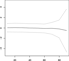
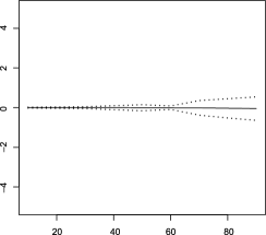
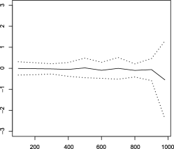
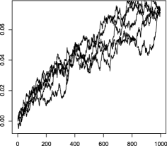
When the $\mathbf{X}_{i}$’s are i.i.d. with a standard normal density, then the result in the above approximation theorem holds with $k=n-1$ implying that $p(\mathbf{X}_{1}^{n-1}=x_{1}^{n-1}|\mathbf{S}_{1,n}=na)=g_{na}(x_{1}^{n-1})$ for all $x_{1}^{n-1}$ in $\mathbb{R}^{n-1}$. This extends to the case when they have an infinitely divisible distribution. However, formula (2) holds true without the error term only in the Gaussian case. Similar exact formulas can be obtained for infinitely divisible distributions using (2.3.1) where no use of tilting is made. Such formulas are used to produce Figures 1, 2, 3 and 4 in order to assess the validity of the selection rule for $k$ in the exponential case.

Remark 4.

The density in (7) is a slight modification of $\pi^{m_{i}}$. The modification from $\pi^{m_{i}}(y_{i+1})$ to $g(y_{i+1}|y_{1}^{i})$ is a small shift in the location parameter depending both on $a$ and on the skewness of $p$, and a change in the variance: large values of $\mathbf{X}_{i+1}$ have smaller weight for large $i$, so that the distribution of $\mathbf{X}_{i+1}$ tends to concentrate around $m_{i}$ as $i$ approaches $k$.

Remark 5.

In Theorem 2, as in Proposition 1, Theorem 8 or Lemma 23, we use an Edgeworth expansion for the density of the normalized sum of the $(n-i)$th row of some triangular array of row-wise independent r.v.’s with a common density. Consider the i.i.d. r.v.’s $\mathbf{X}_{1},\ldots,\mathbf{X}_{n}$ with common density $\pi^{a}(x)$ where $a$ may depend on $n$ but remains bounded. The Edgeworth expansion with respect to the normalized density of $\mathbf{S}_{1,n}$ under $\pi^{a}$ can be derived following closely the proof given, for example, in Feller1971 , page 532 ff., by substituting the cumulants of $p$ by those of $\pi^{a}$. Denote $\varphi_{a}(z)$ the characteristic function of $\pi^{a}(x)$. Clearly for any $\delta>0$ there exists $q_{a,\delta}<1$ such that $|\varphi_{a}(z)|<q_{a,\delta}$ and since $a$ is bounded, $\sup_{n}q_{a,\delta}<1$. Therefore inequality (2.5) in Feller1971 , page 533 holds. With $\psi_{n}$ defined as in Feller1971 , (2.6) holds with $\varphi$ replaced by $\varphi_{a}$ and $\sigma$ by $s(t^{a})$; (2.9) holds, which completes the proof of the Edgeworth expansion in the simple case. The proof is analogous for higher order expansions.

2.3.2 Sampling under the approximation.

Figure 3: $\overline{\operatorname{ERE}}(k)$ (solid line) along with upper and lower bound of $\overline{\operatorname{CI}}(k)$ (dotted line) as a function of $k$ with $n=1000$ and $a$ such that $P_{n}\simeq 10^{-8}$.

Figure 4: $\operatorname{ERE}(k)$ (solid line) along with upper and lower bound of $\operatorname{CI}(k)$ (dotted line) as a function of $k$ with $n=1000$ and $a$ such that $P_{n}\simeq 10^{-8}$.

Applications of Theorem 2 in importance sampling procedures and in Statistics require a reverse result. So assume that $Y_{1}^{k}$ is a random vector generated under $G_{na}$ with density $g_{na}$. Can we state that $g_{na}(Y_{1}^{k})$ is a good approximation for $p_{na}(Y_{1}^{k})$? This holds true. We state a simple lemma in this direction.

Let $\mathfrak{R}_{n}$ and $\mathfrak{S}_{n}$ denote two p.m.’s on $\mathbb{R}^{n}$ with respective densities $\mathfrak{r}_{n}$ and $\mathfrak{s}_{n}$.

Lemma 6

Suppose that for some sequence $\varepsilon_{n}$ which tends to $0$ as $n$ tends to infinity

$$\mathfrak{r}_{n}\bigl{(}Y_{1}^{n}\bigr{)}=\mathfrak{s}_{n}\bigl{(}Y_{1}^{n}\bigr{)}\bigl{(}1+o_{\mathfrak{R}_{n}}(\varepsilon_{n})\bigr{)}$$ (18)

as $n$ tends to $\infty$. Then

$$\mathfrak{s}_{n}\bigl{(}Y_{1}^{n}\bigr{)}=\mathfrak{r}_{n}\bigl{(}Y_{1}^{n}\bigr{)}\bigl{(}1+o_{\mathfrak{S}_{n}}(\varepsilon_{n})\bigr{)}.$$ (19)

Denote

$$A_{n,\varepsilon_{n}}:=\bigl{\{}y_{1}^{n}\dvtx(1-\varepsilon_{n})\mathfrak{s}_{n}\bigl{(}y_{1}^{n}\bigr{)}\leq\mathfrak{r}_{n}\bigl{(}y_{1}^{n}\bigr{)}\leq\mathfrak{s}_{n}\bigl{(}y_{1}^{n}\bigr{)}(1+\varepsilon_{n})\bigr{\}}.$$

It holds for all positive $\delta$,

$$\lim_{n\rightarrow\infty}\mathfrak{R}_{n}(A_{n,\delta\varepsilon_{n}})=1.$$

Write

$$\mathfrak{R}_{n}(A_{n,\delta\varepsilon_{n}})=\int\mathbf{1}_{A_{n,\delta\varepsilon_{n}}}\bigl{(}y_{1}^{n}\bigr{)}\frac{\mathfrak{r}_{n}(y_{1}^{n})}{\mathfrak{s}_{n}(y_{1}^{n})}\mathfrak{s}_{n}\bigl{(}y_{1}^{n}\bigr{)}\,dy_{1}^{n}.$$

Since

$$\mathfrak{R}_{n}(A_{n,\delta\varepsilon_{n}})\leq(1+\delta\varepsilon_{n})\mathfrak{S}_{n}(A_{n,\delta\varepsilon_{n}}),$$

it follows that

$$\lim_{n\rightarrow\infty}\mathfrak{S}_{n}(A_{n,\delta\varepsilon_{n}})=1,$$

which proves the claim.

As a direct by-product of Theorem 2 and Lemma 6 we obtain:

Theorem 7

Assume (K1) and (K2) together with (E1) and (E2). Let $Y_{1}^{k}$ be a sample with density $g_{na}$. It holds that

$$p_{na}\bigl{(}Y_{1}^{k}\bigr{)}=g_{na}\bigl{(}Y_{1}^{k}\bigr{)}\bigl{(}1+o_{G_{na}}\bigl{(}\varepsilon_{n}(\log n)^{2}\bigr{)}\bigr{)}.$$

3 Random walks conditioned by a function of their summands.

This section extends the above results to the case when the conditioning event is written as

$$\mathbf{U}_{1,n}:=u_{1,n}$$ (20)

with

$$\mathbf{U}_{1,n}:=u(\mathbf{X}_{1})+\cdots+u(\mathbf{X}_{n}),$$

where the function $u$ is real valued and the sequence $u_{1,n}/n$ converges. The characteristic function of the random variable $u(\mathbf{X})$ is assumed to belong to $L^{r}$ for some $r\geq 1$. Let $p_{\mathbf{U}}$ denote the density of $\mathbf{U}=u(\mathbf{X})$ and denote $p_{\mathbf{X}}$ the density of $\mathbf{X}$.

Assume

$$\phi_{\mathbf{U}}(t):=E\bigl{[}\exp(t\mathbf{U})\bigr{]}<\infty$$ (21)

for $t$ in a nonempty neighborhood of $0$. Define the functions $m(t)$, $s^{2}(t)$ and $\mu_{3}(t)$ as the first, second and third derivatives of $\log\phi_{\mathbf{U}}(t)$.

Denote

$$\pi_{\mathbf{U}}^{\alpha}(u):=\frac{\exp(tu)}{\phi_{\mathbf{U}}(t)}p_{\mathbf{U}}(u)$$ (22)

with $m(t)=\alpha$, and $\alpha$ belongs to the support of $P_{\mathbf{U}}$, the distribution of $\mathbf{U}$.

We also introduce the family of densities

$$\pi_{u}^{\alpha}(x):=\frac{\exp(tu(x))}{\phi_{\mathbf{U}}(t)}p_{\mathbf{X}}(x).$$ (23)

3.1 Approximation of the density of the runs.

Assume that the sequence $\varepsilon_{n}$ satisfies (E1) and (E2).

Define a density $g_{u_{1,n}}(y_{1}^{k})$ on $\mathbb{R}^{k}$ as follows. Set

$$m_{0}:=u_{1,n}/n$$

and

$$g_{0}(y_{1}|y_{0}):=\pi_{u}^{m_{0}}(y_{1})$$ (24)

with $y_{0}$ arbitrary and, for $1\leq i\leq k-1$, define $g(y_{i+1}|y_{1}^{i})$ recursively. Denote $u_{1,i}:=u(y_{1})+\cdots+u(y_{i})$.

Set $t_{i}$ to be the unique solution of the equation

$$m_{i}:=m(t_{i})=\frac{u_{1,n}-u_{1,i}}{n-i},$$ (25)

and let

$$s_{i}^{2}:=\frac{d^{2}}{dt^{2}}\bigl{(}\log E_{\pi_{\mathbf{U}}^{m_{i}}}\exp(t\mathbf{U})\bigr{)}(0)$$

and

$$\mu_{j}^{i}:=\frac{d^{j}}{dt^{j}}\bigl{(}\log E_{\pi_{\mathbf{U}}^{m_{i}}}\exp(t\mathbf{U})\bigr{)}(0),\qquad j=3,4,$$

which are the second, third and fourth cumulants of $\pi_{\mathbf{U}}^{m_{i}}$. A density $g(y_{i+1}|y_{1}^{i})$ is defined as

$$g\bigl{(}y_{i+1}|y_{1}^{i}\bigr{)}=C_{i}p_{\mathbf{X}}(y_{i+1})\mathfrak{n}\bigl{(}\alpha\beta+m_{0},\beta,u(y_{i+1})\bigr{)}.$$ (26)

Here

$$\alpha = t_{i}+\frac{\mu_{3}^{i}}{2s_{i}^{4}(n-i-1)},$$ (27)

$$\beta = s_{i}^{2}(n-i-1),$$ (28)

and the $C_{i}$ is a normalizing constant.

Set

$$g_{u_{1,n}}\bigl{(}y_{1}^{k}\bigr{)}:=g_{0}(y_{1}|y_{0})\prod_{i=1}^{k-1}g\bigl{(}y_{i+1}|y_{1}^{i}\bigr{)}.$$ (29)

Theorem 8

Assume (K1) and (K2) together with (E1) and (E2). Then (i)

$$p_{u_{1,n}}\bigl{(}Y_{1}^{k}\bigr{)}:=p\bigl{(}\mathbf{X}_{1}^{k}=Y_{1}^{k}|\mathbf{U}_{1,n}=u_{1,n}\bigr{)}=g_{u_{1,n}}\bigl{(}Y_{1}^{k}\bigr{)}\bigl{(}1+o_{P_{u_{1,n}}}\bigl{(}\varepsilon_{n}(\log n)^{2}\bigr{)}\bigr{)}$$

and (ii)

$$p_{u_{1,n}}\bigl{(}Y_{1}^{k}\bigr{)}=g_{u_{1,n}}\bigl{(}Y_{1}^{k}\bigr{)}\bigl{(}1+o_{G_{u_{1,n}}}\bigl{(}\varepsilon_{n}(\log n)^{2}\bigr{)}\bigr{)}.$$

We only sketch the initial step of the proof of (i), which rapidly follows the same path as that in Theorem 2.

As in the proof of Theorem 2, evaluate

$$p(\mathbf{X}_{i+1}=Y_{i+1}|\mathbf{U}_{i+1,n}=u_{1,n}-U_{1,i})$$

$$\qquad=p_{\mathbf{X}}(\mathbf{X}_{i+1}=Y_{i+1})\frac{p_{\mathbf{U}}(\mathbf{U}_{i+2,n}=u_{1,n}-U_{1,i+1})}{p_{\mathbf{U}}(\mathbf{U}_{i+1,n}=u_{1,n}-U_{1,i})}$$

$$\qquad=\frac{p_{\mathbf{X}}(\mathbf{X}_{i+1}=Y_{i+1})}{p_{\mathbf{U}}(\mathbf{U}_{i+1}=u(Y_{i+1}))}p_{\mathbf{U}}\bigl{(}\mathbf{U}_{i+1}=u(Y_{i+1})\bigr{)}\frac{p_{\mathbf{U}}(\mathbf{U}_{i+2,n}=u_{1,n}-U_{1,i+1})}{p_{\mathbf{U}}(\mathbf{U}_{i+1,n}=u_{1,n}-U_{1,i})}.$$

Use the invariance of the conditional density with respect to the change of sampling defined by $\pi_{\mathbf{U}}^{m_{i}}$ to obtain

$$p(\mathbf{X}_{i+1}=Y_{i+1}|\mathbf{U}_{i+1,n}=u_{1,n}-U_{1,i})$$

$$\qquad=\frac{p_{\mathbf{X}}(\mathbf{X}_{i+1}=Y_{i+1})}{p_{\mathbf{U}}(\mathbf{U}_{i+1}=u(Y_{i+1}))}\pi_{\mathbf{U}}^{m_{i}}\bigl{(}\mathbf{U}_{i+1}=u(Y_{i+1})\bigr{)}\frac{\pi_{\mathbf{U}}^{m_{i}}(\mathbf{U}_{i+2,n}=u_{1,n}-U_{1,i+1})}{\pi_{\mathbf{U}}^{m_{i}}(\mathbf{U}_{i+1,n}=u_{1,n}-U_{1,i})}$$

$$\qquad=p_{\mathbf{X}}(\mathbf{X}_{i+1}=Y_{i+1})\frac{e^{t_{i}u(Y_{i+1})}}{\phi_{\mathbf{U}}(t_{i})}\frac{\pi_{\mathbf{U}}^{m_{i}}(\mathbf{U}_{i+2,n}=u_{1,n}-U_{1,i+1})}{\pi_{\mathbf{U}}^{m_{i}}(\mathbf{U}_{i+1,n}=u_{1,n}-U_{1,i})},$$

and proceed via the Edgeworth expansions in the above expression, following verbatim the proof of Theorem 2. We omit details. The proof of (ii) follows from Lemma 6.

We turn to a consequence of Theorem 8.

For all $\delta>0$, let

$$E_{k,\delta}:=\biggl{\{}y_{1}^{k}\in\mathbb{R}^{k}\dvtx\biggl{|}\frac{p_{u_{1,n}}(y_{1}^{k})-g_{u_{1,n}}(y_{1}^{k})}{g_{u_{1,n}}(y_{1}^{k})}\biggr{|}<\delta\biggr{\}},$$

which by Theorem 8 satisfies

$$\lim_{n\rightarrow\infty}P_{u_{1,n}}(E_{k,\delta})=\lim_{n\rightarrow\infty}G_{u_{1,n}}(E_{k,\delta})=1.$$ (30)

It holds that

$$\sup_{C\in\mathcal{B}(\mathbb{R}^{k})}\bigl{|}P_{u_{1,n}}(C\cap E_{k,\delta})-G_{u_{1,n}}(C\cap E_{k,\delta})\bigr{|}$$

$$\qquad\leq\delta\sup_{C\in\mathcal{B}(\mathbb{R}^{k})}\int_{C\cap E_{k,\delta}}g_{u_{1,n}}\bigl{(}y_{1}^{k}\bigr{)}\,dy_{1}^{k}\leq\delta.$$

By (30)

$$\sup_{C\in\mathcal{B}(\mathbb{R}^{k})}\bigl{|}P_{u_{1,n}}(C\cap E_{k,\delta})-P_{u_{1,n}}(C)\bigr{|}<\eta_{n}$$

and

$$\sup_{C\in\mathcal{B}(\mathbb{R}^{k})}\bigl{|}G_{u_{1,n}}(C\cap E_{k,\delta})-G_{u_{1,n}}(C)\bigr{|}<\eta_{n}$$

for some sequence $\eta_{n}\rightarrow 0$; hence

$$\sup_{C\in\mathcal{B}(\mathbb{R}^{k})}\bigl{|}P_{u_{1,n}}(C)-G_{u_{1,n}}(C)\bigr{|}<\delta+2\eta_{n}$$

for all positive $\delta$. Applying Scheffé’s lemma, we have proved:

Theorem 9

Under the hypotheses of Theorem 8 the total variation distance between $P_{u_{1,n}}$ and $G_{u_{1,n}}$ goes to $0$ as $n$ tends to infinity, and

$$\lim_{n\rightarrow\infty}\int\bigl{|}p_{u_{1,n}}\bigl{(}y_{1}^{k}\bigr{)}-g_{u_{1,n}}\bigl{(}y_{1}^{k}\bigr{)}\bigr{|}\,dy_{1}^{k}=0.$$

Remark 10.

This result is to be compared with Theorem 1.6 in DiaconisFreedman1988 and Theorem 2.15 in DemboZeitouni1996 which provides a rate for this convergence for small $k$’s under some additional conditions on the moment generating function of $\mathbf{U}$.

3.1.1 Approximation under other sampling schemes.

In statistical applications the r.v.’s $Y_{i}$’s in Theorems 2 and 8 may in certain cases be sampled under some other distribution than $P_{na}$ or $G_{na}$.

Consider the following situation.

The model consists of an exponential family $\mathcal{P}:=\{P_{\theta,\eta},(\theta,\eta)\in\mathcal{N}\}$ defined on $\mathbb{R}$ with canonical parametrization $(\theta,\eta)$ and sufficient statistics $(t,u)$ defined on $\mathbb{R}$ through the densities

$$p_{\theta,\eta}(x):=\frac{dP_{\theta,\eta}(x)}{dx}=\exp\bigl{(}\theta t(x)+\eta u(x)-K(\theta,\eta)\bigr{)}h(x).$$ (31)

We assume that both $\theta$ and $\eta$ belong to $\mathbb{R}$. The natural parameter space $\mathcal{N}$ is a convex set in $\mathbb{R}^{2}$ defined as the domain of

$$k(\theta,\eta):=\exp\bigl{(}K(\theta,\eta)\bigr{)}=\int\exp\bigl{(}\theta t(x)+\eta u(x)\bigr{)}h(x)\,dx.$$

For the statistician, $\theta$ is the parameter of interest whereas $\eta$ is a nuisance one. The unknown parameter of the i.i.d. sample $\mathbf{X}_{1}^{n}:=(\mathbf{X}_{1},\ldots,\mathbf{X}_{n})$ observed as $X_{1}^{n}:=(X_{1},\ldots,X_{n})$ is $(\theta_{T},\eta_{T})$.

Conditioning on a sufficient statistic for the nuisance parameter produces a new exponential family which is free of $\eta$. For any $\theta$ denote $\widehat{\eta}_{\theta}$ the MLE of $\eta_{T}$ in model (31) parametrized in $\eta$, when $\theta$ is fixed. A classical solution for the estimation of $\theta_{T}$ consists in maximizing the likelihood

$$L\bigl{(}\theta|X_{1}^{n}\bigr{)}:=\prod_{i=1}^{n}p_{\theta,\widehat{\eta}_{\theta}}(X_{i})$$

with respect to $\theta$. This approach produces satisfactory results when $\widehat{\eta}_{\theta}$ is a consistent estimator of $\eta_{\theta}$. However for curved exponential families, it may happen that for some $\theta$ the likelihood

$$L_{\theta}\bigl{(}\eta|X_{1}^{n}\bigr{)}:=\prod_{i=1}^{n}p_{\theta,\eta}(X_{i})$$

is multimodal with respect to $\eta$ which may produce misestimation in $\widehat{\eta}_{\theta}$, leading in turn to inconsistency in the resulting estimates of $\theta_{T}$; see Sundberg2009 .

Consider $g_{u_{1,n},(\theta,\eta)}$ defined in (29) for fixed $(\theta,\eta)$, with $u_{1,n}:=u(X_{1})+\cdots+u(X_{n})$. Since $u_{1,n}$ is sufficient for $\eta$, $p_{u_{1,n},(\theta,\eta)}$ is independent of $\eta$ for all $k$. Assume at present that the density $g_{u_{1,n},(\theta,\eta)}$ on $\mathbb{R}^{k}$ approximates $p_{u_{1,n},(\theta,\eta)}$ on the sample $X_{1}^{n}$ generated under $(\theta_{T},\eta_{T})$; it follows then that inserting any value $\eta_{0}$ in (29) does not change the value of the resulting likelihood

$$L_{\eta_{0}}\bigl{(}\theta|X_{1}^{k}\bigr{)}:=g_{u_{1,n},(\theta,\eta_{0})}(X_{i}).$$

Optimizing $L_{\eta_{0}}(\theta|X_{1}^{k})$ with respect to $\theta$ produces a consistent estimator of $\theta_{T}$. We refer to BroniatowskiCaron2012Exp for examples and discussion.

Let $\mathbf{Y}_{1}^{n}$ be i.i.d. copies of $\mathbf{Z}$ with distribution $Q$ and density $q$; assume that $Q$ satisfies the Cramér condition $\int(\exp(tx))q(x)\,dx<\infty$ for $t$ in a nonempty neighborhood of $0$. Let $\mathbf{V}_{1,n}:=u(\mathbf{Y}_{1})+\cdots+u(\mathbf{Y}_{n})$, and define

$$q_{u_{1,n}}\bigl{(}y_{1}^{k}\bigr{)}:=q\bigl{(}\mathbf{Y}_{1}^{k}=y_{1}^{k}|\mathbf{V}_{1,n}=u_{1,n}\bigr{)}$$

with distribution $Q_{u_{1,n}}$. The following theorem then holds:

Theorem 11

Assume (K1) and (K2) together with (E1) and (E2). Then, with the same hypotheses and notation as in Theorem 8,

$$p\bigl{(}\mathbf{X}_{1}^{k}=Y_{1}^{k}|\mathbf{U}_{1,n}=u_{1,n}\bigr{)}=g_{u_{1,n}}\bigl{(}Y_{1}^{k}\bigr{)}\bigl{(}1+o_{Q_{u_{1,n}}}\bigl{(}\varepsilon_{n}(\log n)^{2}\bigr{)}\bigr{)}.$$

Also the total variation distance between $Q_{u_{1,n}}$ and $P_{u_{1,n}}$ goes to $0$ as $n$ tends to infinity.

It is enough to check that Lemmas 21, 22 and 23 hold when $\mathbf{Y}$ satisfies the Cramér condition.

Remark 12.

In the previous discussion $Q=P_{\theta_{T,}\eta_{T}}$ and $\mathbf{X}_{1}^{n}$ are independent copies of $\mathbf{X}$ with distribution $P_{\theta,\eta_{0}}$.

3.2 For how long is the approximation valid?

This section provides a rule leading to an effective choice of the crucial parameter $k$ in order to achieve a given accuracy bound for the relative error in Theorem 8(ii). The accuracy of the approximation is measured through

$$\operatorname{ERE}(k):=E_{G_{u_{1,n}}}1_{D_{k}}\bigl{(}Y_{1}^{k}\bigr{)}\frac{p_{u_{1,n}}(Y_{1}^{k})-g_{u_{1,n}}(Y_{1}^{k})}{p_{u_{1,n}}(Y_{1}^{k})}$$ (32)

and

$$\operatorname{VRE}(k):=\operatorname{Var}_{G_{u_{1,n}}}1_{D_{k}}\bigl{(}Y_{1}^{k}\bigr{)}\frac{p_{u_{1,n}}(Y_{1}^{k})-g_{u_{1,n}}(Y_{1}^{k})}{p_{u_{1,n}}(Y_{1}^{k})}$$ (33)

respectively, the expectation and the variance of the relative error of the approximating scheme when evaluated on

$$D_{k}:=\bigl{\{}y_{1}^{k}\in\mathbb{R}^{k}\mbox{ such that }\bigl{|}g_{u_{1,n}}\bigl{(}y_{1}^{k}\bigr{)}/p_{u_{1,n}}\bigl{(}y_{1}^{k}\bigr{)}-1\bigr{|}<\delta_{n}\bigr{\}}$$

with $\varepsilon_{n}(\log n)^{2}/\delta_{n}\rightarrow 0$ and $\delta_{n}\rightarrow 0$; therefore $G_{u_{1,n}}(D_{k})\rightarrow 1$. The r.v.’s $Y_{1}^{k}$ are sampled under $g_{u_{1,n}}$. Note that the density $p_{u_{1,n}}$ is usually unknown. The argument is somehow heuristic and informal; nevertheless the rule is simple to implement and provides good results. We assume that the set $D_{k}$ can be substituted by $\mathbb{R}^{k}$ in the above formulas, therefore assuming that the relative error has bounded variance, which would require quite a lot of work to be proved under appropriate conditions, but which seems to hold, at least in all cases considered by the authors. We keep the above notation omitting therefore any reference to $D_{k}$.

Consider a two-sigma confidence bound for the relative accuracy for a given $k$, defining

$$\operatorname{CI}(k):=\bigl{[}\operatorname{ERE}(k)-2\sqrt{\operatorname{VRE}(k)},\operatorname{ERE}(k)+2\sqrt{\operatorname{VRE}(k)}\bigr{]}.$$

Let $\delta$ denote an acceptance level for the relative accuracy. Accept $k$ until $\delta$ belongs to $\operatorname{CI}(k)$. For such $k$, the relative accuracy is certified up to the level $5\%$ roughly.

The calculation of $\operatorname{VRE}(k)$ and $\operatorname{ERE}(k)$ should be carried out as follows.

Write

$$\operatorname{VRE}(k)^{2} = E_{P_{\mathbf{X}}}\biggl{(}\frac{g_{u_{1,n}}^{3}(Y_{1}^{k})}{p_{u_{1,n}}(Y_{1}^{k})^{2}p_{\mathbf{X}}(Y_{1}^{k})}\biggr{)}$$

$${}-E_{P_{\mathbf{X}}}\biggl{(}\frac{g_{u_{1,n}}^{2}(Y_{1}^{k})}{p_{u_{1,n}}(Y_{1}^{k})p_{\mathbf{X}}(Y_{1}^{k})}\biggr{)}^{2}$$

$$=: A-B^{2}.$$

By the Bayes formula,

$$p_{u_{1,n}}\bigl{(}Y_{1}^{k}\bigr{)}=p_{\mathbf{X}}\bigl{(}Y_{1}^{k}\bigr{)}\frac{np(\mathbf{U}_{k+1,n}/(n-k)=m(t_{k}))}{(n-k)p(\mathbf{U}_{1,n}/n=u_{1,n}/n)}.$$ (34)

The following lemma holds; see Jensen1995 and Richter1957 .

Lemma 13

Let $\mathbf{U}_{1},\ldots,\mathbf{U}_{n}$ be i.i.d. random variables with common density $p_{\mathbf{U}}$ on $\mathbb{R}$ and satisfying the Cramér conditions with m.g.f. $\phi_{\mathbf{U}}$. Then with $m(t)=u$,

$$p(\mathbf{U}_{1,n}/n=u)=\frac{\sqrt{n}\phi_{\mathbf{U}}^{n}(t)\exp(-ntu)}{s(t)\sqrt{2\pi}}\bigl{(}1+o(1)\bigr{)}$$

when $|u|$ is bounded.

Introduce

$$D:=\biggl{[}\frac{\pi_{\mathbf{U}}^{m_{0}}(m_{0})}{p_{\mathbf{U}}(m_{0})}\biggr{]}^{n}$$

and

$$N:=\biggl{[}\frac{\pi_{\mathbf{U}}^{m_{k}}(m_{k})}{p_{\mathbf{U}}(m_{k})}\biggr{]}^{(n-k)}$$

with $m_{k}$ defined in (25) and $m_{0}=u_{1,n}/n$. Define $t$ by $m(t)=m_{0}$. By (34) and Lemma 13 it holds that

$$p_{u_{1,n}}\bigl{(}Y_{1}^{k}\bigr{)}=\sqrt{\frac{n}{n-k}}p_{\mathbf{X}}\bigl{(}Y_{1}^{k}\bigr{)}\frac{D}{N}\frac{s(t)}{s(t_{k})}\bigl{(}1+o_{P_{u_{1,n}}}(1)\bigr{)}.$$

The approximation of $A$ is obtained through Monte Carlo simulation. Define

$$A\bigl{(}Y_{1}^{k}\bigr{)}:=\frac{n-k}{n}\biggl{(}\frac{g_{u_{1,n}}(Y_{1}^{k})}{p_{\mathbf{X}}(Y_{1}^{k})}\biggr{)}^{3}\biggl{(}\frac{N}{D}\biggr{)}^{2}\frac{s^{2}(t_{k})}{s^{2}(t)},$$ (35)

and simulate $L$ i.i.d. samples $Y_{1}^{k}(l)$, each one made of $k$ i.i.d. replicates under $p_{\mathbf{X}}$. Set

$$\widehat{A}:=\frac{1}{L}\sum_{l=1}^{L}A\bigl{(}Y_{1}^{k}(l)\bigr{)}.$$

We use the same approximation for $B$. Define

$$B\bigl{(}Y_{1}^{k}\bigr{)}:=\sqrt{\frac{n-k}{n}}\biggl{(}\frac{g_{u_{1,n}}(Y_{1}^{k})}{p_{\mathbf{X}}(Y_{1}^{k})}\biggr{)}^{2}\biggl{(}\frac{N}{D}\biggr{)}\frac{s(t_{k})}{s(t)}$$ (36)

and

$$\widehat{B}:=\frac{1}{L}\sum_{l=1}^{L}B\bigl{(}Y_{1}^{k}(l)\bigr{)}$$

with the same $Y^{k}_{l}(l)$’s as above.

Set

$$\overline{\operatorname{VRE}}(k):=\widehat{A}-(\widehat{B})^{2},$$ (37)

which is a suitable approximation of $\operatorname{VRE}(k)$.

The curve $k\rightarrow\overline{\operatorname{ERE}}(k)$ is a proxy for (32) and is obtained through

$$\overline{\operatorname{ERE}}(k):=1-\widehat{B}.$$

A proxy of $\operatorname{CI}(k)$ can now be defined as

$$\overline{\operatorname{CI}}(k):=\bigl{[}\overline{\operatorname{ERE}}(k)-2\sqrt{\overline{\operatorname{VRE}}(k)},\overline{\operatorname{ERE}}(k)+2\sqrt{\overline{\operatorname{VRE}}(k)}\bigr{]}.$$ (38)

We now check the validity of the above approximation, comparing $\overline{\operatorname{CI}}(k)$ with $\operatorname{CI}(k)$ on a toy case.

Consider $u(x)=x$. The case when $p_{\mathbf{X}}$ is a centered exponential distribution with variance $1$ allows for an explicit evaluation of $\operatorname{CI}(k)$ making no use of Lemma 13. The conditional density $p_{na}$ is calculated analytically, the density $g_{na}$ is obtained through (10), hence providing a benchmark for our proposal. The terms $\widehat{A}$ and $\widehat{B}$ are obtained by Monte Carlo simulation following the algorithm presented below. Figures 1, 2 and 3, 4 show the increase in $\delta$ w.r.t. $k$ in the large deviation range, with $a$ such that $P(\mathbf{S}_{1,n}>na)\simeq 10^{-8}$. We have considered two cases, when $n=100$ and when $n=1000$. These figures show that the approximation scheme is quite accurate, since the relative error is fairly small. Also they show that $\overline{\operatorname{ERE}}$ and $\overline{\operatorname{CI}}$ provide good tools for the assessing the value of $k$.

Algorithms 1 and 2 produce the curve $k\rightarrow\overline{\operatorname{CI}}(k)$. The resulting $k=k_{\delta}$ is the longest run length for which $g_{u_{1,n}}$ a good proxy for $p_{u_{1,n}}$.

Input : $y_{1}^{k}$, $p_{\mathbf{X}}$, $n$, $u_{1,n}$

Output : $g_{u_{1,n}}(y_{1}^{k})$

Initialization : 

$t_{0}\leftarrow m^{-1}(m_{0})$;

$g_{0}(y_{1}|y_{0})\leftarrow$ (24);

Procedure : 

for $i\leftarrow 1$ to $k-1$ do  $m_{i}\leftarrow$ (25);

$t_{i}\leftarrow m^{-1}(m_{i})$ $*$;

$\alpha\leftarrow$ (27);

$\beta\leftarrow$ (28);

Calculate $C_{i}$;

$g(y_{i+1}|y_{1}^{i})\leftarrow$ (26); end Compute $g_{u_{1,n}}(y_{1}^{k})\leftarrow$ (29);

Return : $g_{u_{1,n}}(y_{1}^{k})$

Algorithm 1 Evaluation of $g_{u_{1,n}}(y_{1}^{k})$.

The calculation of $g_{u_{1,n}}(y_{1}^{k})$ above requires the value of

$$C_{i}=\biggl{(}\int p_{\mathbf{X}}(x)\mathfrak{n}\bigl{(}\alpha\beta+m_{0},\beta,u(x)\bigr{)}\,dx\biggr{)}^{-1}.$$

This can be done through Monte Carlo simulation.

Input :  $p_{\mathbf{X}}$, $\delta$, $n$, $u_{1,n}$, $L$

Output : $k_{\delta}$

Initialization : $k=1$

Procedure : 

while $\delta\notin\overline{\operatorname{CI}}(k)$ do  for $l\leftarrow 1$ to $L$ do  Simulate $Y_{1}^{k}(l)$ i.i.d. with density $p_{\mathbf{X}}$;

$A(Y_{1}^{k}(l)):={}$(35) using Algorithm 1;

$B(Y_{1}^{k}(l)):={}$(36) using Algorithm 1; end Calculate $\overline{\operatorname{CI}}(k)\leftarrow{}$(38);

$k:=k+1$; end

Return : $k_{\delta}:=k$

Algorithm 2 Calculation of $k_{\delta}$.

Input : $p$, $\mu$, $\sigma^{2}$

Output : $Y$

Initialization : 

Select a density $f$ on $[0,1]$ and a positive constant $K$ such that $p(\mathfrak{N}^{-1}(x))\leq Kf(x)$ for all $x$ in $[0,1]$

Procedure :  while $Z<$ $p(\mathfrak{N}^{-1}(X))$ do 

Simulate $X$ with density $f$;

Simulate $U$ uniform on $[0,1]$ independent of $X$;

Compute $Z:=KUf(X)$; end

Return : $Y:=\mathfrak{N}^{-1}(X)$

Algorithm 3 Simulation of $Y$ with density proportional to $p(x)\mathfrak{n}(\mu,\sigma^{2},x)$.

Remark 14.

Solving $t_{i}=m^{-1}(m_{i})$ might be difficult. It may happen that the inverse function of $m$ is at hand, but even when $p_{\mathbf{X}}$ is the Weibull density and $u(x)=x$, this is not the case. We can replace step $\ast$ by

$$t_{i+1}:=t_{i}-\frac{(m(t_{i})+u_{i})}{(n-i)s^{2}(t_{i})}.$$

Indeed since

$$m(t_{i+1})-m(t_{i})=-\frac{1}{n-i}\bigl{(}m(t_{i})+u_{i}\bigr{)}$$

use a first order approximation to derive that $t_{i+1}$ can be substituted by $\tau_{i+1}$ defined as

$$\tau_{i+1}:=t_{i}-\frac{1}{(n-i)s^{2}(t_{i})}\bigl{(}m(t_{i})+u_{i}\bigr{)}.$$

When $\lim_{n\rightarrow\infty}u_{1,n}/n=Eu(\mathbf{X})$, the values of the function $s^{2}(\cdot)$ are close to $\operatorname{Var}[u(\mathbf{X})]$, and the above approximation is appropriate. For the large deviation case, the same argument applies, since $s^{2}(t_{i})$ keeps close to $s^{2}(t^{a})$.

Input : $p_{\mathbf{X}}$, $\delta$, $n$, $u_{1,n}$

Output : $Y_{1}^{k}$

Initialization : 

Set $k\leftarrow k_{\delta}$ with Algorithm 2;

$t_{0}\leftarrow=m^{-1}(m_{0})$;

Procedure : 

Simulate $Y_{1}$ with density (24);

$u_{1,1}\leftarrow u(Y_{1})$;

for $i\leftarrow 1$ to $k-1$ do 

$m_{i}\leftarrow{}$(25);

$t_{i}\leftarrow m^{-1}(m_{i})$;

$\alpha\leftarrow{}$(27);

$\beta\leftarrow{}$(28);

Simulate $Y_{i+1}$ with density $g(y_{i+1}|y_{1}^{i})$ using Algorithm 3;

$u_{1,i+1}\leftarrow u_{1,i}+u(Y_{i+1})$; end

Return : $Y_{1}^{k}$

Algorithm 4 Simulation of a sample $Y_{1}^{k}$ with density $g_{u_{1,n}}$.

3.2.1 Simulation of typical paths of a random walk under a conditioning point.

By Theorem 8(ii), $g_{u_{1,n}}$ and the density of $p_{u_{1,n}}$ approach each other on a family of subsets of $\mathbb{R}^{k}$ which contain the typical paths of the random walk under the conditional density with probability going to $1$ as $n$ increases. By Lemma 6 large sets under $P_{u_{1,n}}$ are also large sets under $G_{u_{1,n}}$. It follows that long runs of typical paths under $p_{u_{1,n}}$ can be simulated as typical paths under $g_{u_{1,n}}$ defined in (29) at least for large $n$.

The simulation of a sample $X_{1}^{k}$ with $g_{u_{1,n}}$ can be fast and easy when $\lim_{n\rightarrow\infty}u_{1,n}/n=Eu(\mathbf{X})$. Indeed the r.v. $\mathbf{X}_{i+1}$ with density $g(x_{i+1}|x_{1}^{i})$ is obtained through a standard acceptance-rejection algorithm. The values of the parameters which appear in the Gaussian component of $g(x_{i+1}|x_{1}^{i})$ in (7) are easily calculated, and the dominating density can be chosen for all $i$ as $p_{\mathbf{X}}$. The constant in the acceptance rejection algorithm is then $1/\sqrt{2\pi\beta}$. This is in contrast with the case when the conditioning value is in the range of a large deviation event, that is, $\lim_{n\rightarrow\infty}u_{1,n}/n\neq Eu(\mathbf{X})$, which appears in a natural way in importance sampling estimation for rare event probabilities; then MCMC techniques can be used.

Figure 5: Trajectories in the normal case for $P_{n}=10^{-2}$.

Figure 6: Trajectories in the normal case for $P_{n}=10^{-8}$.

Denote $\mathfrak{N}$ the c.d.f. of a normal variate with parameter $(\mu,\sigma^{2})$ and $\mathfrak{N}^{-1}$ its inverse.

Remark 15.

Simulation of $Y_{1}$ can be performed through the method suggested in BarbeBroniatowski1999 .

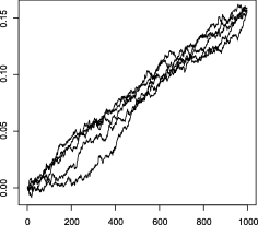
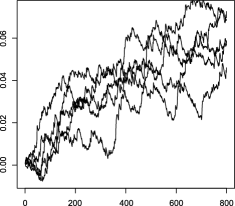
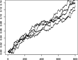
Figures 5, 6, 7 and 8 present a number of simulations of random walks conditioned on their sum with $n=1000$ when $u(x)=x$. In the Gaussian case, when the approximating scheme is known to be optimal up to $k=n-1$, the simulation is performed with $k=999$ and two cases are considered: the moderate deviation case is assumed to be modeled when $P(\mathbf{S}_{1,n}>na)=10^{-2}$ (Figure 5); that this range of probability is in the “moderate deviation” range is a commonly assessed statement among statisticians. The large deviation case pertains to $P(\mathbf{S}_{1,n}>na)=10^{-8}$ (Figure 6). The centered exponential case with $n=1000$ and $k=800$ is presented in Figures 7 and 8, under the same events.

Figure 7: Trajectories in the exponential case for $P_{n}=10^{-2}$.

Figure 8: Trajectories in the exponential case for $P_{n}=10^{-8}$.

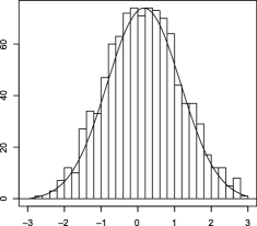
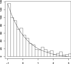
In order to check the accuracy of the approximation, Figures 9, 10 (normal case, $n=1000$, $k=999$) and Figures 11, 12 (centered exponential case, $n=1000$, $k=800$) present the histograms of the simulated $\mathbf{X}_{i}$’s together with the tilted densities at point $a$ which are known to be the limit density of $\mathbf{X}_{1}$ conditioned on $\mathcal{E}_{n}$ in the large deviation case, and to be equivalent to the same density in the moderate deviation case, as can be deduced from ERmakov2006 . The tilted density in the Gaussian case is the normal with mean $a$ and variance $1$; in the centered exponential case the tilted density is an exponential density on $(-1,\infty)$ with parameter $1/(1+a)$.

Figure 9: Histogram of the $\mathbf{X}_{i}$’s in the normal case with $n=1000$ and $k=999$ for $P_{n}=10^{-2}$. The curve represents the associated tilted density.

Figure 10: Histogram of the $\mathbf{X}_{i}$’s in the normal case with $n=1000$ and $k=999$ for $P_{n}=10^{-8}$. The curve represents the associated tilted density.

Figure 11: Histogram of the $\mathbf{X}_{i}$’s in the exponential case with $n=1000$ and $k=800$ for $P_{n}=10^{-2}$. The curve represents the associated tilted density.

Figure 12: Histogram of the $\mathbf{X}_{i}$’s in the exponential case with $n=1000$ and $k=800$ for $P_{n}=10^{-8}$. The curve represents the associated tilted density.

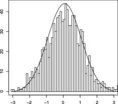
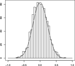
Consider now the case when $u(x)=x^{2}$. Figure 13 presents the case when $\mathbf{X}$ is $N(0,1)$, $n=1000,k=800$, $P(\mathbf{U}_{1,n}=u_{1,n})\simeq 10^{-2}$. We present the histograms of the $X_{i}$’s together with the graph of the corresponding tilted density; when $\mathbf{X}$ is $N(0,1)$, then $\mathbf{X}^{2}$ is $\chi^{2}$. It is well known that when $u_{1,n}/n$ is fixed to be larger than $1$, then the limit distribution of $\mathbf{X}_{1}$ conditioned on $(\mathbf{U}_{1,n}=u_{1,n})$ tends to $N(0,a)$ which is the Kullback–Leibler projection of $N(0,1)$ on the set of all probability measures $Q$ on $\mathbb{R}$ with $\int x^{2}\,dQ(x)=a:=\lim_{n\rightarrow\infty}u_{1,n}/n$. This distribution is precisely $g_{0}(y_{1}|y_{0})$ defined above. Also consider (26); the expansion using the definitions (27) and (28) prove that as $n\rightarrow\infty$ the dominating term in $g_{i}(y_{i+1}|y_{1}^{i})$ is precisely $N(0,m_{0})$, and the terms including $y_{i+1}^{4}$ in the exponential stemming from $\mathfrak{n}(\alpha\beta+m_{0},\beta,u(y_{i+1}))$ are of order $O(1/(n-i))$; the terms depending on $y_{1}^{i}$ are of smaller order. The fit which is observed in Figure 13 is in accordance with the above statement in the LDP range (when $\lim_{n\rightarrow\infty}u_{1,n}/n\neq 1$), and with the MDP approximation when $\lim_{n\rightarrow\infty}u_{1,n}/n=1$ and $\lim\inf_{n\rightarrow\infty}(u_{1,n}-n)/\sqrt{n}\neq 0$, following ERmakov2006 .

Figure 13: Histogram of the $\mathbf{X}_{i}$’s in the normal case with $n=1000$, $k=800$ and $u(x)=x^{2}$ for $P_{n}=10^{-2}$. The curve represents the associated tilted density.

4 Conditioning on large sets.

The approximation of the density

$$p_{A_{n}}\bigl{(}\mathbf{X}_{1}^{k}=Y_{1}^{k}\bigr{)}:=p\bigl{(}\mathbf{X}_{1}^{k}=Y_{1}^{k}|\mathbf{U}_{1,n}\in A_{n}\bigr{)}$$

of the runs $\mathbf{X}_{1}^{k}$ under large sets $(\mathbf{U}_{1,n}\in A_{n})$ for Borel sets $A_{n}$ with nonempty interior follows from the above results through integration. Here, in the same vein as previously, $Y_{1}^{k}$ is generated under $P_{A_{n}}$. An application of this result for the evaluation of rare event probabilities through importance sampling is briefly presented in the next section. The present section pertains to the large deviation case.

4.1 Conditioning on a large set defined through the density of its dominating point.

We focus on cases when $(\mathbf{U}_{1,n}\in A_{n})$ can be expressed as $(\mathbf{U}_{1,n}/n\in A)$ where $A$ is a fixed Borel set (independent of $n$) with essential infimum $\alpha$ larger than $E\mathbf{U}$ and which can be described as a “thin” or “thick” Borel set according to its local density at point $\alpha$.

The starting point is the approximation of $p_{nv}$ on $\mathbb{R}^{k}$ for large values of $k$ under the conditioning point

$$\mathbf{U}_{1,n}/n=v$$

when $v$ belongs to $A$. Denote $g_{nv}$ the corresponding approximation defined in (29). It holds that

$$p_{nA}\bigl{(}x_{1}^{k}\bigr{)}=\int_{A}p_{nv}\bigl{(}\mathbf{X}_{1}^{k}=x_{1}^{k}\bigr{)}p(\mathbf{U}_{1,n}/n=v|\mathbf{U}_{1,n}\in nA)\,ds.$$ (39)

In contrast with the classical importance sampling approach for this problem we do not consider the dominating point approach, but merely realize a sharp approximation of the integrand at any point of the domain $A$ and consider the dominating contribution of all those distributions in the evaluation of the conditional density $p_{nA}$. A similar point of view has been considered in BarbeBroniatowski2004 for sharp approximations of Laplace-type integrals in $\mathbb{R}^{d}$.

Turning to (39) it appears that what is needed is a sharp approximation for

$$p(\mathbf{U}_{1,n}/n=v|\mathbf{U}_{1,n}\in nA)=\frac{p(\mathbf{U}_{1,n}/n=v){\mathbh{1}}_{A}(v)}{P(\mathbf{U}_{1,n}\in nA)}$$ (40)

with some uniformity for $v$ in $A$. We will assume that $A$ is bounded above in order to avoid further regularity assumptions on the distribution of $\mathbf{U}$.

Recall that the essential infimum essinf$A=\alpha$ of the set $A$ with respect to the Lebesgue measure is defined through

$$\alpha:=\inf\bigl{\{}x\dvtx\mbox{ for all }\varepsilon>0,\bigl{|}[x,x+\varepsilon]\cap A\bigr{|}>0\bigr{\}}$$

with $\inf\varnothing:=-\infty$.

We assume that $\alpha>-\infty$, which is tantamount to saying that we do not consider very thin sets (e.g., not Cantor-type sets).

The density of the point $\alpha$ in $A$ will not be measured in the ordinary way, through

$$d(\alpha):=\lim_{\varepsilon\rightarrow 0}\frac{|A\cap[\alpha-\varepsilon,\alpha+\varepsilon]|}{\varepsilon},$$

but through the more appropriate quantity

$$M(t):=t\int_{A-\alpha}e^{-ty}\,dy,\qquad t>0.$$

For any set $A$, $0\leq M(t)\leq 1$. If there exists an interval $[\alpha,\alpha+\varepsilon]\subset A$, then $\lim_{t\rightarrow\infty}M(t)=1$. As an example, for a self similar set $A:=A_{p}$ defined as $A_{p}:=\bigcup_{n\in\mathbb{Z}}p^{n}I_{p}$ where $p>2$ and $I_{p}:=[(p-1)/p,1]$, it holds that $0=\mathrm{essinf}A_{p}$ and $pA_{p}=A_{p}$. Consequently for any $t\geq 0$, $M(tp)=M(t)$ and $M(tp)=M(t)$ for all $t\geq 0$; it follows that

$$\inf_{1\leq u\leq p}M(u)=\lim\inf_{t\rightarrow\infty}M(t)\leq\lim\sup_{t\rightarrow\infty}M(t)=\sup_{1\leq u\leq p}M(u).$$

Define

$$M_{n}(t):=M(nt)/t=\int_{A-\alpha}e^{-ty}\,dy$$

and

$$\Psi_{n}(t):=n\log\phi_{\mathbf{U}}(t)+\log M_{n}(t)-n\alpha t$$

for all $t>0$ such that $\phi_{\mathbf{U}}(t)$ is finite. We borrow from BarbeBro2000 the following results.

Define $\mu_{n}(t):=(1/n)\log M_{n}(t)$ which is for all $n\geq 1$ a decreasing function of $t$ on $(0,\infty)$, and which is negative for large $n$. Also $\mu_{n}^{\prime}(t)=\mu_{1}^{\prime}(nt)$ and $\mu_{1}^{\prime}$ are nondecreasing on $(0,\infty)$.

Let $\overline{\mu}:=\lim_{t\rightarrow\infty}\mu_{1}^{\prime}(t)$ and $\underline{\mu}:=\lim_{t\rightarrow 0}\mu_{1}^{\prime}(t)$. Then according to BarbeBro2000 the following holds:

Lemma 16

Under the above notation and hypotheses, the equation$\Psi_{n}^{\prime}(t)=0$ has a unique solution $t_{n}$ in $(0,t_{0})$ for $\alpha$ in $(E\mathbf{U}+\overline{\mu},\infty)$ where $t_{0}:=\sup\{t\dvtx\phi_{\mathbf{U}}(t)<\infty\}$. Furthermore if $\alpha>E\mathbf{U}+\underline{\mu}$, then there exists a compact set $K\subset(0,t_{0})$ such that $t_{n}\in K$ for all $n$.

Assume that $\alpha>E\mathbf{U}+\underline{\mu}$. Define $\psi_{n}(t):=\Psi_{n}^{\prime\prime}(t)$, and suppose that for any $\lambda>0$,

$$\lim_{n\rightarrow\infty}\sup_{|u|<\lambda}\frac{\psi_{n}(t_{n}+{u}/{\sqrt{\psi_{n}(t_{n})}})}{\psi_{n}(t_{n})}=1,$$ (41)

where $t_{n}$ is a solution of $\Psi_{n}^{\prime}(t)=0$ in the range $(0,t_{0})$. It can be proved that (41) holds, for example, when $t\rightarrow\log M(t)/t$ is a regularly varying function at infinity with index $\rho\in(0,1)$, that is, $\log M(t)/t\in\mathcal{R}_{\rho}(\infty)$; see BarbeBro2000 , Lemma 2.2.

We also assume that

$$\lim\sup_{t\rightarrow\infty}t\bigl{(}\log M(t)\bigr{)}<\infty,$$ (42)

which holds, for example, when $\log(M(t)/t)\in\mathcal{R}_{\rho}(\infty)$, for $0\leq\rho<1$.

Theorem 2.1 in BarbeBro2000 provides a general result to be inserted in (40); we take the occasion to correct a misprint in this result.

Theorem 17

Assume (41) and (42) together with the aforementioned conditions on the r.v. $\mathbf{U}$. Then for $\alpha>E\mathbf{U}+\underline{\mu}$,

$$P(\mathbf{U}_{1,n}\in nA)=\frac{\phi_{\mathbf{U}}^{n}(t_{n})M_{n}(t_{n})e^{-nt_{n}\alpha}}{\sqrt{\psi_{n}(t_{n})}\sqrt{2\pi}}\bigl{(}1+o(1)\bigr{)}\qquad\mbox{as }n\rightarrow\infty,$$ (43)

with $t_{n}$ satisfying $\Psi_{n}^{\prime}(t)=0$ provided that the function $x\rightarrow P(\mathbf{U}_{1,n}\in nA+x)$ is nonincreasing for $n$ large enough. In particular, this last condition holds if [(iii)]

(Petrov): $A=(\alpha,\infty)$ or $A=[\alpha,\infty)$; in this case $M_{n}(t)=1/t$; note that in this case the classical result is slightly different, since

$$P(\mathbf{U}_{1,n}>na)=\frac{\phi_{\mathbf{U}}^{n}(t^{a})e^{-nt^{a}a}}{t^{a}s(t^{a})\sqrt{2\pi}}\bigl{(}1+o(1)\bigr{)}\qquad\mbox{as }n\rightarrow\infty$$

with $m(t^{a})=a$ and $a>E\mathbf{U}$; this is readily seen to be equivalent to (43) when $A=(a,\infty)$.

$\mathbf{U}$ has a symmetric unimodal distribution.

$\mathbf{U}$ has a strongly unimodal distribution.

The shape of $A$ near $\alpha$ is reflected in the behavior of the function $M(t)$ for large values of $t$. As such, the larger the $n$, the more relevant is the shape of $A$ near $\alpha$.

Note further that $M_{n}(t)e^{-nt\alpha}=\int_{A}e^{-nty}\,dy$ from which we see that $\alpha$ plays no role in (43). Hence $\alpha$ can be replaced by any number $\gamma$ such that $\int_{A-\gamma}e^{-ty}\,dy$ converges. Further $t_{n}$ is independent of $\alpha$. The so-called dominating point $\alpha$ of $A$ can therefore be defined as

$$\alpha:=\lim_{t\rightarrow\infty}\log\int_{A}e^{-ty}\,dy.$$

In order to examine further the role played in (43) by the regularity of $A$ near its essential infimum $\alpha$, introduce the pointwise Hölder dimension of $A$ at $\alpha$ as

$$\delta(\alpha):=\frac{\log G(\varepsilon)}{-\log\varepsilon},$$

where

$$G(\varepsilon):=\bigl{|}A\cap[\alpha,\alpha+\varepsilon]\bigr{|}\qquad\mbox{for positive }\varepsilon.$$

We refer to Proposition 2.1 in BarbeBro2000 for a set of Abel–Tauber-type results which link the properties of $M(t)$ at infinity with those of $G$ at $0$. For example, it follows that $G(\varepsilon)\sim\varepsilon^{\delta(\alpha)}$ (as $\varepsilon\rightarrow 0$) if and only if $M(t)\sim ct^{-\delta(\alpha)+1}\Gamma(1+\delta(\alpha))$ (as $t\rightarrow\infty$). Consequently if $M_{n}(t)\rightarrow 1$ as $t\rightarrow\infty$, then $M(t)\sim t$ as $t\rightarrow\infty$ and $G(\varepsilon)\sim\varepsilon$ as $\varepsilon\rightarrow 0$.

Asymptotic formulas for the numerator in (40) are well known and have a long history, going back to Richter1957 . It holds that

$$p(\mathbf{U}_{1,n}/n=v)=\frac{\sqrt{n}e^{nvt^{v}}\phi_{\mathbf{U}}(t^{v})}{\sqrt{2\pi}s(t^{v})}\bigl{(}1+o(1)\bigr{)}\qquad\mbox{as }n\rightarrow\infty$$ (44)

with $t^{v}$ defined as $m(t^{v})=v$.

Plugging in (44) and (43) in (39) provides an expression for the density of the runs. For applications the only relevant case is developed in the following paragraph.

4.2 Conditioning on a thick set.

In the case when $A=(a,\infty)$ or with $a>Eu(\mathbf{X})$ or, more generally, when $A$ is a thick set in a neighborhood of its essential infimum [i.e., when $\lim_{t\rightarrow\infty}M(t)=1$] a simple asymptotic evaluation for (40) when $A$ is unbounded can be obtained. Indeed an expansion of the ratio yields

$$p(\mathbf{U}_{1,n}/n=v|\mathbf{U}_{1,n}>na)=\bigl{(}nt\exp\bigl{(}-nt(v-a)\bigr{)}\bigr{)}{\mathbh{1}}_{A}(v)\bigl{(}1+o(1)\bigr{)}$$ (45)

with $m(t)=a$, indicating that $\mathbf{U}_{1,n}/n$ is roughly exponentially distributed on $A$ with expectation $a+1/nt$. This result is used in Section 5 in order to derive estimators of some rare event probabilities through importance sampling.

In order to obtain a sharp approximation for $p_{nA}(\mathbf{X}_{1}^{k}=Y_{1}^{k})$ it is necessary to introduce an interval $(a,a+c_{n})$ which contains the principal part of the integral (39).

Let $c_{n}$ denote a positive sequence such that the following condition (C) holds:

$$\lim_{n\rightarrow\infty}nc_{n} = \infty,$$

$$\sup_{n\geq 1}\frac{nc_{n}}{(n-k)} < \infty$$

and denote $c$ the current term $c_{n}$.

Define on $\mathbb{R}^{k}$ the density

$$g_{nA}\bigl{(}y_{1}^{k}\bigr{)}$$

(46)

$$\qquad:=\frac{nm^{-1}(a)\int_{a}^{a+c}g_{nv}(y_{1}^{k})(\exp(-nm^{-1}(a)(v-a)))\,dv}{1-\exp(-nm^{-1}(a)c)}.$$

The density

$$\frac{nm^{-1}(a)(\exp(-nm^{-1}(a)(v-a))){\mathbh{1}}_{(a,a+c)}(v)}{1-\exp(-nm^{-1}(a)c)},$$ (47)

which appears in (4.2) approximates $p(\mathbf{U}_{1,n}/n=v|a<\mathbf{U}_{1,n}/n<a+c)$. Furthermore due to Theorem 8 $g_{nv}(Y_{1}^{k})$ approximates $p_{nv}(Y_{1}^{k})$ when $Y_{1}^{k}$ results from sampling under $P_{nA}$. For a discussion on the maximal value of $k$ for which a given relative accuracy is attained, see BroniatowskiCaron2011IS .

The variance function $V$ of the distribution of $\mathbf{U}$ is defined on the span of $\mathbf{U}$ through

$$v\rightarrow V(v):=s^{2}\bigl{(}m^{-1}(v)\bigr{)}.$$

Denote (V) the condition

$$\sup_{n\geq 1}\sqrt{n}\int_{a}^{\infty}V^{\prime}(v)\bigl{(}\exp\bigl{(}-nm^{-1}(a)(v-a)\bigr{)}\bigr{)}\,dv<\infty.$$

Theorem 18

Assume (E1), (E2), (C), (V). Then for any positive $\delta<1$:

(i)

$$p_{nA}\bigl{(}\mathbf{X}_{1}^{k}=Y_{1}^{k}\bigr{)}=g_{nA}\bigl{(}Y_{1}^{k}\bigr{)}\bigl{(}1+o_{P_{nA}}(\delta_{n})\bigr{)}$$ (48)

and (ii)

$$p_{nA}\bigl{(}\mathbf{X}_{1}^{k}=Y_{1}^{k}\bigr{)}=g_{nA}\bigl{(}Y_{1}^{k}\bigr{)}\bigl{(}1+o_{G_{nA}}(\delta_{n})\bigr{)},$$ (49)

where

$$\delta_{n}:=\max\bigl{(}\varepsilon_{n}(\log n)^{2},\bigl{(}\exp(-nc)\bigr{)}^{\delta}\bigr{)}.$$ (50)

See the Appendix.

Most distributions used in statistics satisfy (V); numerous papers have focused on the properties of variance functions and classification of distributions; see, for example, LetacMora and references therein.

Corollary 19

Under the hypotheses of Theorem 18 the total variation distance between $P_{nA}$ and $G_{nA}$ goes to $0$ as $n$ tends to infinity, that is,

$$\lim_{n\rightarrow\infty}\int\bigl{|}p_{nA}\bigl{(}y_{1}^{k}\bigr{)}-g_{nA}\bigl{(}y_{1}^{k}\bigr{)}\bigr{|}\,dy_{1}^{k}=0.$$

5 Applications.

5.1 Rao–Blackwellization of estimators.

This example illustrates the role of Theorem 8 in statistical inference; the conditioning event is local, in the range where $\lim_{n\rightarrow\infty}u_{1,n}/n=Eu(\mathbf{X})$.

In statistics the following situation is often encountered. A model $\mathcal{P}$ consists of a family of densities $p_{\theta}$ where the parameter $\theta$ is assumed to belong to $\mathbb{R}^{d}$, and a sample of i.i.d. r.v.’s $\mathbf{X}_{1}^{n}$ is observed, with each of the $\mathbf{X}_{i}$’s having density $p_{\theta_{T}}$ where $\theta_{T}$ is unknown; denote $X_{1},\ldots,X_{n}$ the observed data set. Let $\mathbf{U}_{1,n}:=u(\mathbf{X}_{1})+\cdots+u(\mathbf{X}_{n})$ and let $u_{1,n}:=u(X_{1})+\cdots+u(X_{n})$, which usually satisfies $\lim_{n\rightarrow\infty}u_{1,n}/n=Eu(\mathbf{X})$. A preliminary estimator $\widehat{\theta}(\mathbf{X}_{1}^{n})$ is chosen, which may have the advantage of being easily computable, at the cost of having poor efficiency, approaching $\theta_{T}$ loosely in terms of the MSE. The famous Rao–Blackwell theorem asserts that the MSE of the conditional expectation of $\widehat{\theta}(\mathbf{X}_{1}^{n})$ given the observed value $u_{1,n}$ of any statistic improves on the MSE of $\widehat{\theta}(\mathbf{X}_{1}^{n})$. When $u_{1,n}$ is sufficient for $\theta$ the reduction is maximal, leading to the unbiased minimal variance estimator for $\theta_{T}$ when $\widehat{\theta}(\mathbf{X}_{1}^{n})$ is unbiased (Lehmann–Scheffé theorem).

The conditional density $p_{u_{1,n}}(x_{1}^{n}):=p(\mathbf{X}_{1}^{n}=x_{1}^{n}|\mathbf{U}_{1,n}=u_{1,n})$ is usually unknown, and Rao–Blackwellization of estimators cannot be performed in many cases. Simulations of long runs of length $k=k_{n}$ under a proxy of $p_{u_{1,n}}(x_{1}^{k})$ provide an easy way to improve the preliminary estimator, averaging values of $\widehat{\theta}((X_{1}^{k})(l))_{1\leq l\leq L}$ where the samples $(X_{1}^{k}(l))$’s are obtained under the approximation of $p_{u_{1,n}}(x_{1}^{k})$ and $L$ runs are performed.

Consider the Gamma density

$$f_{\rho,\theta}(x):=\frac{\theta^{-\rho}}{\Gamma(\rho)}x^{\rho-1}\exp\biggl{(}-\frac{x}{\theta}\biggr{)}\qquad\mbox{for }x>0.$$ (51)

As $\rho$ varies in $\mathbb{R}^{+}$ and $\theta$ is positive, the density belongs to an exponential family $\gamma_{r,\theta}$ with parameters $r:=\rho-1$ and $\theta$, and sufficient statistics are $t(x):=\log x$ and $u(x):=x$, respectively, for $r$ and $\theta$. Given an i.i.d. sample $X_{1}^{n}:=(X_{1},\ldots,X_{n})$ with density $\gamma_{r_{T},\theta_{T}}$ the resulting sufficient statistics are, respectively, $t_{1,n}:=\log X_{1}+\cdots+\log X_{n}$ and $u_{1,n}:=X_{1}+\cdots+X_{n}$. We consider the parametic model $(\gamma_{r_{T},\theta},\theta\geq{0})$ assuming $r_{T}$ known.

Definition (29) shows that $g_{u_{1,n}}$ depends on the unknown parameter $\theta_{T}$. It can be seen that $u_{1,n}$ is nearly sufficient for $\theta$ in $g_{u_{1,n}}$ in the sense that the value of $g_{u_{1,n}}(X_{1}^{k})$ does not vary when $\theta_{T}$ is substituted by any other value $\theta$ of the parameter and the $X_{i}$’s are generated under any density $\gamma_{r_{T},\theta^{\prime}}$ (see BroniatowskiCaron2012Exp ) this is indeed in agreement with the statement of Theorem 11. Hence on one hand $,u_{1,n}$ can be used to obtain improved estimators of $\theta_{T}$ and on the other hand, $g_{u_{1,n}}$ can be used to simulate samples distributed under a proxy of $p_{u_{1,n}}$ using any $\theta$ in lieu of $\theta_{T}$ in (29), as is done in the following procedure:

A first unbiased estimator of $\theta_{T}$ is chosen as

$$\widehat{\theta}_{2}:=\frac{X_{1}+X_{2}}{2r_{T}}.$$

Given an i.i.d. sample $X_{1}^{n}$ with density $\gamma_{r_{T},\theta_{T}}$ the Rao–Blackwellized estimator of $\widehat{\theta}$ is defined as

$$\theta_{RB,2}:=E(\widehat{\theta}_{2}|\mathbf{U}_{1,n})$$

whose variance is less than $\operatorname{Var}\widehat{\theta}_{2}$.

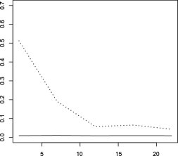
Consider $k=2$ in $g_{u_{1,n}}(y_{1}^{k})$, and let $(Y_{1},Y_{2})$ be distributed according to $g_{u_{1,n}}(y_{1}^{2})$. Replicates of $(Y_{1},Y_{2})$ induce an estimator of $\theta_{RB,2}$ for fixed $u_{1,n}$. Iterating on the simulation of the runs $X_{1}^{n}$ produces for $n=100$ an i.i.d. sample of $\theta_{RB,2}$’s from which $\operatorname{Var}\theta_{RB,2}$ is estimated. The resulting variance shows a net improvement with respect to the estimated variance of $\widehat{\theta}_{2}$. It is of some interest to investigate this gain in efficiency as the number of terms involved in $\widehat{\theta}_{k}$ increases together with $k$. As $k$ approaches $n$ the variance of $\widehat{\theta}_{k}$ approaches the Cramér–Rao bound. Figure 14 shows the decay of the variance of $\widehat{\theta}_{k}$. We note that whatever the value of $k$ the estimated value of the variance of $\theta_{RB,k}$ is constant, and is quite close to the Cramér–Rao bound. This is indeed an illustration of Lehmann–Scheffé’s theorem.

Figure 14: Variance of $\widehat{\theta}_{k}$, the initial estimator (dotted line), along with the variance of $\theta_{RB,k}$, the Rao–Blackwellized estimator (solid line) with $n=100$ as a function of $k$.

5.2 Importance sampling for rare event probabilities.

Here we consider the application of the approximating scheme under a conditioning event defined through a large set, where this event is also on the large deviation scale. A development of the present section is presented in BroniatowskiCaron2011IS and in Section 3 of Caronetal2013 ; see also BroniatowskiRitov2009 . Consider the estimation of the large deviation probability for the mean of $n$ i.i.d. r.v.’s $u(\mathbf{X}_{i})$ satisfying the conditions of this paper. This is a benchmark problem in the study of rare events; we refer to Bucklew2004 for the background of this section.

Let $u_{1,n}:=na$ for fixed $a$ larger than $Eu(\mathbf{X})$. The probability to be estimated is

$$P_{n}:=P(\mathbf{U}_{1,n}>u_{1,n}).$$

The importance sampling procedure substitutes the empirical estimator

$$\widehat{P}_{n} := \frac{1}{L}\sum_{l=1}^{L}\mathbh{1}\bigl{(}\mathbf{U}_{1,n}(l)>u_{1,n}\bigr{)}$$

$$= \frac{1}{L}\sum_{l=1}^{L}\mathbh{1}\Biggl{(}\sum_{i=1}^{n}u\bigl{(}\mathbf{X}_{i}(l)\bigr{)}>u_{1,n}\Biggr{)}$$

by

$$\quad P_{n}^{\mathrm{IS},g}:=\frac{1}{L}\sum_{l=1}^{L}\frac{p(u(\mathbf{X}_{1}(l)))\cdots p(u(\mathbf{X}_{n}(l)))}{g(u(\mathbf{X}_{1}(l))\cdots u(\mathbf{X}_{n}(l)))}\mathbh{1}\Biggl{(}\sum_{i=1}^{n}u\bigl{(}\mathbf{X}_{i}(l)\bigr{)}>u_{1,n}\Biggr{)}.$$ (53)

In the above display (5.2) the sample $\mathbf{X}_{1}^{n}(l)$ is generated under i.i.d. sampling with distribution $P_{\mathbf{X}}$ and the $L$ samples are i.i.d. In display (53) the sample $\mathbf{X}_{1}^{n}(l)$ is generated under the density $g$ on $\mathbb{R}^{n}$ (under which the $\mathbf{X}_{i}$’s may not be independent). The $L$ samples $\mathbf{X}_{1}^{n}(l)$ are i.i.d.

It is well known that the optimal sampling density is

$$p_{\mathrm{opt}}\bigl{(}x_{1}^{n}\bigr{)}:=p\bigl{(}\mathbf{X}_{1}^{n}=x_{1}^{n}|\mathbf{U}_{1,n}>u_{1,n}\bigr{)},$$

which is not achievable since it presumes a known $P_{n}$. This optimal sampling density produces the zero variance estimator $P_{n}$ itself with $L=1$. However approximating $p_{\mathrm{opt}}(x_{1}^{n})$ sharply at least on the first $k$ coordinates for large $k$ produces a large hit rate for the importance sampling procedure, and pushes the importance factor toward 1.

Define the sampling density $g$ on $\mathbb{R}^{n}$ as

$$g\bigl{(}x_{1}^{n}\bigr{)}:=g_{nA}\bigl{(}x_{1}^{k}\bigr{)}\prod_{i=k+1}^{n}\pi_{u}^{a}(x_{i}),$$

where $g_{nA}$ is defined in (4.2), and $\pi_{u}^{a}$ is the density defined in (23). The approximating density $g_{nA}$ has been used to simulate the $k$ first $\mathbf{X}_{i}$’s and the remaining $n-k$’s are i.i.d. with the classical tilted density. The classical IS scheme coincides with the present one with the difference that $k=1$ and $g_{A_{n}}(x_{1})=\pi_{u}^{a}(x_{1})$, that is, simulating under an i.i.d. sampling scheme with common density $\pi_{u}^{a}$.

Figure 15: Ratio of the empirical value of the MSE of the adaptive estimate w.r.t. the empirical MSE of the i.i.d. twisted one (dotted line) along with the true value of this ratio (solid line) as a function of $k$.

Simulation under $g_{nA}$ is performed through a double step procedure: In the first step, randomize the value of $\mathbf{U}_{1,n}/n$ on $(a,+\infty)$ according to a proxy of its distribution conditioned on $\mathbf{U}_{1,n}>na$; hence simulate a random variable $S$ on $(a,+\infty)$ with density

$$p_{S}(s):=nm^{-1}(a_{n})\bigl{(}\exp\bigl{(}-nm^{-1}(a)(s-a)\bigr{)}\bigr{)}{\mathbh{1}}_{(a,+\infty)}(s).$$ (54)

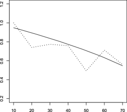
Then plug in $nS$ in lieu of $u_{1,n}$ in (29) and iterate. This is equivalent to considering each point in the target set as a dominating point, weighted by its conditional density under $(\mathbf{U}_{1,n}>na)$. Simulation of $S$ under (54) instead of (47) is slightly suboptimal but much simpler. It can be proved that the MSE of the estimate of $P_{n}$ in this new IS sampling scheme is reduced by a factor $\sqrt{(n-k)/n}$ with respect to the classical scheme when calculated on large subsets of $\mathbb{R}^{k}$; see BroniatowskiCaron2011IS . Figure 15 shows, in a simple case, the ratio of the empirical value of the MSE of the adaptive estimate w.r.t. the empirical MSE of the i.i.d. twisted one, in the exponential case with $P_{n}=10^{-2}$ and $n=100$. The value of $k$ grows from $k=0$ (i.i.d. twisted sample) to $k=70$ (according to the rule presented in BroniatowskiCaron2011IS ). This ratio stabilizes to $\sqrt{n-k}/\sqrt{n}$ for $L=2000$. The abscissa is $k$ and the solid line is $k\rightarrow\sqrt{n-k}/\sqrt{n}$.

Remark 20.

In the present context, Dupuis and Wang DupuisWang2004 have shown that i.i.d. sampling schemes can produce “rogue paths” which may alter the properties of the estimate, and the estimation of its variance. They consider an i.i.d. random sample $X_{1}^{n}$ where $X_{1}$ has a normal distribution $N(1,1)$ and

$$\mathcal{E}_{n}:=\biggl{\{}x_{1}^{n}\dvtx\frac{x_{1}+\cdots+x_{n}}{n}\in A\biggr{\}},$$

where $A=(-\infty,a)\cup(b,+\infty)$ with $a<1<b$. The quantity to be estimated is $P(\mathcal{E}_{n})$.

Assuming that $a+b<2$, the standard i.i.d. IS scheme introduces the dominating point $b$ and the family of i.i.d. tilted r.v.’s with common $N(b,1)$ distribution. “Rogue paths” generated under $N(b,1)$ may hit the set $(-\infty,a)$ with small probability under the sampling scheme, hence producing a very large importance factor. The resulting variance of the estimate is very sensitive with respect to these values, as exemplified in their Table 1, page 24. Simulation of paths according to $G_{nS}$ with $S$ defined in (54) produces their constructive samples which yield both a hit rate close to 100% and an importance factor close to $P(\mathcal{E}_{n})$. We refer to BroniatowskiCaron2011IS for discussion and examples. We also note that Dupis and Wang DupuisWang2004 propose an adaptive tilting scheme, based on the product of the $\pi^{m_{i}}$, $1\leq i\leq n$, which yields an efficient IS algorithm.

Appendix

For clarity the current term $a_{n}$ is denoted $a$ in all proofs.

.3 Three lemmas pertaining to the partial sum under its final value.

We state three lemmas which describe some functions of the random vector $\mathbf{X}_{1}^{n}$ conditioned on $\mathcal{E}_{n}$. The r.v. $\mathbf{X}$ is assumed to have expectation $0$ and variance $1$.

Lemma 21

It holds that $E_{P_{na}}(\mathbf{X}_{1})=a,E_{P_{na}}(\mathbf{X}_{1}\mathbf{X}_{2})=a{}^{2}+O(\frac{1}{n})$,$E_{P_{na}}(\mathbf{X}_{1}^{2})=s^{2}(t)+a{}^{2}+O(\frac{1}{n})$ where $m(t)=a$.

Using

$$p_{na}(\mathbf{X}_{1}=x)=\frac{p_{\mathbf{S}_{2,n}}(na-x)p_{\mathbf{X}_{1}}(x)}{p_{\mathbf{S}_{1,n}}(na)}=\frac{\pi_{\mathbf{S}_{2,n}}^{a}(na-x)\pi_{\mathbf{X}_{1}}^{a}(x)}{\pi_{\mathbf{S}_{1,n}}^{a}(na)},$$

normalizing both $\pi_{\mathbf{S}_{2,n}}^{a}(na-x)$ and $\pi_{\mathbf{S}_{1,n}}^{a}(na)$ and making use of a first order Edgeworth expansion in those expressions yields $E_{P_{na}}(\mathbf{X}_{1}^{2})=s^{2}(t)+a{}^{2}+O(\frac{1}{n})$. A similar expansion for the joint density $p_{na}(\mathbf{X}_{1}=x,\mathbf{X}_{2}=y)$, with the same tilted distribution $\pi^{a}$ produces the limit expression of $E_{P_{na}}(\mathbf{X}_{1}\mathbf{X}_{2})$.

Lemma 22

Assume (E1). Then (i) $\max_{1\leq i\leq k}|m_{i}|=a+o_{P_{na}}(\varepsilon_{n})$. Also (ii) $\max_{1\leq i\leq k}s_{i}^{2}$, $\max_{1\leq i\leq k}\mu_{3}^{i}$ and $\max_{1\leq i\leq k}\mu_{4}^{i}$ tend in $P_{na}$ probability to the variance, skewness and kurtosis of $\pi^{\underline{a}}$ where $\underline{a}:=\lim_{n\rightarrow\infty}a_{n}$.

(i) Define

$$V_{i+1} := m(t_{i})-a$$

$$= \frac{S_{i+1,n}}{n-i}-a.$$

We state that

$${\max_{0\leq{i\leq{k-1}}}|V_{i+1}|=}o_{P_{na}}(\varepsilon_{n}),$$ (55)

namely for all positive $\delta$

$$\lim_{n\rightarrow\infty}P_{na}\Bigl{(}\max_{0\leq{i\leq{k-1}}}|V_{i+1}|>\delta\varepsilon_{n}\Bigr{)}=0,$$

which we obtain following the proof of Kolmogorov maximal inequality. Define

$$A_{i}:=\bigl{(}\bigl{(}|V_{i+1}|\geq\delta\varepsilon_{n}\bigr{)}\mbox{ and }\bigl{(}|V_{j}|<\delta\varepsilon_{n}\mbox{ for all }j<i+1\bigr{)}\bigr{)}$$

from which

$$\Bigl{(}\max_{0\leq{i}\leq{k-1}}|V_{i+1}|>\delta\varepsilon_{n}\Bigr{)}=\bigcup_{i=0}^{k-1}A_{i}.$$

It holds that

$$E_{P_{na}}V_{k}^{2} = \int_{\cup A_{i}}V_{k}^{2}\,dP_{na}+\int_{(\cup A_{i})^{c}}V_{k}^{2}\,dP_{na}$$

$$\geq {\int_{\cup A_{i}}}\bigl{(}{V_{i}^{2}+2}(V_{k}-V_{i})V_{i}\bigr{)}\,{dP_{na}+\int_{(\cup A_{i})^{c}}}\bigl{(}{V_{i}^{2}+2}(V_{k}-V_{i})V_{i}\bigr{)}\,{d}P_{na}$$

$$\geq \int_{\cup A_{i}}V_{i}^{2}\,dP_{na}$$

$$\geq \delta^{2}\varepsilon_{n}^{2}{\sum_{j=0}^{k-1}P_{na}(A_{j})}$$

$$= \delta^{2}\varepsilon_{n}^{2}P_{na}\Bigl{(}{\max_{0\leq{i}\leq{k-1}}|V_{i+1}|>}\delta\varepsilon_{n}\Bigr{)}.$$

The third line above follows from $EV_{i}(V_{k}-V_{i})=0$ which is proved below. Hence

$$P_{na}\Bigl{(}{\max_{0\leq{i}\leq{k-1}}|V_{i+1}|>}\delta\varepsilon_{n}\Bigr{)}\leq\frac{\operatorname{Var}_{P_{na}}(V_{k})}{\delta^{2}\varepsilon_{n}^{2}}=\frac{1}{\delta^{2}\varepsilon_{n}^{2}(n-k)}\bigl{(}1+o(1)\bigr{)},$$

where we used Lemma 21; therefore (55) holds under (E1). Direct calculation yields $E_{P_{na}}(V_{i}(V_{k}-V_{i}))={0}$, which completes the proof of (i).

(ii) follows from (i) since $\lim_{n\rightarrow\infty}\max_{1\leq i\leq k}m(t_{i})=\underline{a}$.

We also need the order of magnitude of $\max(|\mathbf{X}_{1}|,\ldots,|\mathbf{X}_{k}|)$ under $P_{na}$ which is stated in the following result.

Lemma 23

It holds that $\max(|\mathbf{X}_{1}|,\ldots,|\mathbf{X}_{n}|)=O_{P_{na}}(\log n)$.

Set $|\mathbf{X}_{1}|:=\mathbf{X}_{i}^{-}+\mathbf{X}_{i}^{+}$ with $\mathbf{X}_{i}^{-}:=-\min(0,\mathbf{X}_{i})$, $\mathbf{X}_{i}^{+}:=\break\max(0,\mathbf{X}_{i})$; it is enough to prove that $\max_{i}\mathbf{X}_{i}^{-}=O_{P_{na}}(\log n)$ and $\max_{i}\mathbf{X}_{i}^{+}=O_{P_{na}}(\log n)$. Since $E[\exp(t\mathbf{X})]$ is finite in a nonempty neighborhood of $0$ so are $E[\exp(t\mathbf{X}^{-})]$ and $E[\exp(t\mathbf{X}^{+})]$. We hence prove the lemma for positive r.v.’s $\mathbf{X}_{i}$ ’s only.

Denote $a$ the current term of the sequence $a_{n}$. For all $t$ it holds that

$$P_{na}\bigl{(}\max(\mathbf{X}_{1},\ldots,\mathbf{X}_{n})>t\bigr{)} \leq nP_{na}(\mathbf{X}_{n}>t)$$

$$= n\int_{t}^{\infty}\pi^{a}(\mathbf{X}_{n}=u)\frac{\pi^{a}(\mathbf{S}_{1,n-1}=na-u)}{\pi^{a}(\mathbf{S}_{1,n}=na)}\,du.$$

Let $\tau$ be such that $m(\tau)=a$. Denote $s:=s(\tau)$. Center and normalize both $\mathbf{S}_{1,n}$ and $\mathbf{S}_{1,n-1}$with respect to the density $\pi^{a}$ in the last line above, denoting $\overline{\pi_{n}^{a}}$ the density of $\overline{\mathbf{S}_{1,n}}:=(\mathbf{S}_{1,n}-na)/s\sqrt{n}$ when $\mathbf{X}$ has density $\pi^{a}$ with mean $a$ and variance $s^{2}$, we obtain

$$P_{na}\bigl{(}\max(\mathbf{X}_{1},\ldots,\mathbf{X}_{n})>t\bigr{)}$$

$$\qquad\leq n\frac{\sqrt{n}}{\sqrt{n-1}}$$

$$\qquad\quad{}\times\int_{t}^{\infty}\pi^{a}(\mathbf{X}_{n}=u)\frac{\overline{\pi_{n-1}^{a}}(\overline{\mathbf{S}_{1,n-1}}=(na-u-(n-1)a)/(s\sqrt{n-1}))}{\overline{\pi_{n}^{a}}(\overline{\mathbf{S}_{1,n}}=0)}\,du.$$

Under the sequence of densities $\pi^{a}$ the triangular array $(\mathbf{X}_{1},\ldots,\mathbf{X}_{n})$ obeys a first order Edgeworth expansion

$$P_{na}\bigl{(}\max(\mathbf{X}_{1},\ldots,\mathbf{X}_{n})>t\bigr{)}$$

$$\qquad\leq n\frac{\sqrt{n}}{\sqrt{n-1}}\int_{t}^{\infty}\pi^{a}(\mathbf{X}_{n}=u)\frac{\mathfrak{n}((a-u)/s\sqrt{n-1})\mathbf{P}(u,i,n)+o(1)}{\mathfrak{n}(0)+o(1)}\,du$$

$$\qquad\leq n\mathit{Cst}\int_{t}^{\infty}\pi^{a}(\mathbf{X}_{n}=u)\,du$$

for some constant $\mathit{Cst}$ independent of $n$ and $\tau$ and

$$\mathbf{P}(u,i,n):=1+P_{3}\bigl{(}(a-u)/s\sqrt{n-1}\bigr{)},$$

where $P_{3}(x)=\frac{\mu_{3}}{6s^{3}}(x^{3}-3x)$ is the third Hermite polynomial; $s^{2}$ and $\mu_{3}$ are the second and third centered moments of $\pi^{a}$. We have used the fact that the sequence $a$ converges to bound all moments of the tilted densities $\pi^{a}$. We used uniformity on $u$ in the remaining term of the Edgeworth expansions. Making use of the Chernoff inequality to bound $\Pi^{a}(\mathbf{X}_{n}>t)$,

$$P_{na}\bigl{(}\max(\mathbf{X}_{1},\ldots,\mathbf{X}_{n})>t\bigr{)}\leq n\mathit{Cst}\frac{\Phi(t+\lambda)}{\Phi(t)}e^{-\lambda t}$$

for any $\lambda$ such that $\phi(t+\lambda)$ is finite. For $t$ such that

$$t/\log n\rightarrow\infty$$

it holds that

$$P_{na}\bigl{(}\max(\mathbf{X}_{1},\ldots,\mathbf{X}_{n})<t\bigr{)}\rightarrow 1,$$

which proves the lemma.

.4 Proof of the approximations resulting from Edgeworth expansions in Theorem 2.

We complete the calculation leading to (15) and (16).

Set $Z_{i+1}:=(m_{i}-Y_{i+1})/s_{i}\sqrt{n-i-1}$.

It then holds that

$$\overline{\pi_{n-i-1}}(Z_{i+1})$$

$$\qquad=\mathfrak{n}(Z_{i+1})\left[\matrix{\displaystyle 1+\frac{1}{\sqrt{n-i-1}}P_{3}(Z_{i+1})+\frac{1}{n-i-1}P_{4}(Z_{i+1})\vspace*{2pt}\cr\displaystyle+\frac{1}{(n-i-1)^{3/2}}P_{5}(Z_{i+1})}\right]$$ (56)

$$\qquad\quad{}+O_{P_{na}}\biggl{(}\frac{P_{5}(Z_{i+1})}{(n-i-1)^{3/2}}\biggr{)}.$$

We perform an expansion in $\mathfrak{n}(Z_{i+1})$ up to order $3$, with a first order term $\mathfrak{n}(-Y_{i+1}/(s_{i}\sqrt{n-i-1}))$, namely

$$\mathfrak{n}(Z_{i+1})$$

$$\qquad=\mathfrak{n}\bigl{(}-Y_{i+1}/(s_{i}\sqrt{n-i-1})\bigr{)}$$ (57)

$$\qquad\quad{}\times\pmatrix{\displaystyle 1+\frac{Y_{i+1}m_{i}}{s_{i}^{2}(n-i-1)}+\frac{m_{i}^{2}}{2s_{i}^{2}(n-i-1)}\biggl{(}\frac{Y_{i+1}^{2}}{s_{i}^{2}(n-i-1)}-1\biggr{)}\vspace*{2pt}\cr\displaystyle+\frac{m_{i}^{3}}{6s_{i}^{3}(n-i-1)^{3/2}}\frac{\mathfrak{n}^{(3)}({Y^{\ast}}/{(s_{i}\sqrt{n-i-1})})}{\mathfrak{n}(-Y_{i+1}/(s_{i}\sqrt{n-i-1}))}},$$

where $Y^{\ast}=\frac{1}{s_{i}\sqrt{n-i-1}}(-Y_{i+1}+\theta m_{i})$ with $|\theta|<1$.

Lemmas 22 and 23 provide the orders of magnitude of the random terms in the above displays when sampling under $P_{na}$.

Use those lemmas to obtain

$$\frac{Y_{i+1}m_{i}}{s_{i}^{2}(n-i-1)}=\frac{Y_{i+1}}{n-i-1}\bigl{(}a+o_{P_{na}}(\varepsilon_{n})\bigr{)}$$ (58)

and

$$\frac{m_{i}^{2}}{s_{i}^{2}(n-i-1)}=\frac{1}{n-i-1}\bigl{(}a+o_{P_{na}}(\varepsilon_{n})\bigr{)}^{2}.$$

Also when (E1) and (E2) holds, then the dominant terms in the bracket in (.4) are precisely those in the two displays just above. This yields

$$\mathfrak{n}(Z_{i+1})=\mathfrak{n}\biggl{(}\frac{-Y_{i+1}}{s_{i}\sqrt{n-i-1}}\biggr{)}\pmatrix{\displaystyle 1+\frac{aY_{i+1}}{s_{i}^{2}(n-i-1)}-\frac{a^{2}}{2s_{i}^{2}(n-i-1)}\vspace*{2pt}\cr\displaystyle+\frac{o_{P_{na}}(\varepsilon_{n}\log n)}{n-i-1}}.$$

We now need a precise evaluation of the terms in the Hermite polynomials in (.4). This is achieved using Lemmas 22 and 23 which provide uniformity on $i$ between $1$ and $k=k_{n}$ in all terms depending on the sample path $Y_{1}^{k}$. The Hermite polynomials depend upon the moments of the underlying density $\pi^{m_{i}}$. Since $\overline{\pi_{1}^{m_{i}}}$ has expectation $0$ and variance $1$ the terms corresponding to $P_{1}$ and $P_{2}$ vanish. For up to order 4 polynomials, write $P_{3}(x)=\frac{\mu_{3}^{(i)}}{6(s_{i})^{3}}H_{3}(x)$, $P_{4}(x)=\frac{(\mu_{3}^{i})^{2}}{72(s_{i})^{6}}H_{6}(x)+\frac{\mu_{4}^{(i,n)}-3(s_{i})^{4}}{24(s_{i})^{4}}H_{4}(x)$ with $H_{3}(x):=x^{3}-3x$, $H_{4}(x):=x^{4}-6x^{2}+3$ and $H_{6}(x):=x^{6}-15x^{4}+45x^{2}-15$.

Using Lemma 22 it appears that the terms in $x^{j}$, $j\geq 3$ in $P_{3}$ and $P_{4}$ will play no role in the asymptotic behavior in (.4) with respect to the constant term in $P_{4}$ and the term in $x$ from $P_{3}$. Indeed substituting $x$ by $Z_{i+1}$ and dividing by $n-i-1$, the term in $x^{2}$ in $P_{4}$ is $O_{P_{na}}(\log n)^{2}/(n-i)^{2}$ where we have used Lemma 22. These terms are of smaller order than the term $-3x$ in $P_{3}$ which is $-\frac{\mu_{3}^{i}}{2s_{i}^{4}(n-i-1)}(a-Y_{i+1})=\frac{1}{n-i-1}O_{P_{na}}(\log n)$.

It holds that

$$\frac{P_{3}(Z_{i+1})}{\sqrt{n-i-1}} = -\frac{\mu_{3}^{i}}{2s_{i}^{4}(n-i-1)}(m_{i}-Y_{i+1})$$

$${}+\frac{\mu_{3}^{i}(m_{i}-Y_{i+1})^{3}}{6(s_{i})^{6}(n-i-1)^{2}},$$

which yields

$$\frac{P_{3}(Z_{i+1})}{\sqrt{n-i-1}}=-\frac{\mu_{3}^{i}}{2s_{i}^{4}(n-i-1)}(a-Y_{i+1})+\frac{O_{P_{na}}(\log n)^{3}}{(n-i-1)^{2}}.$$ (59)

For the term of order $4$ it holds that

$$\frac{P_{4}(Z_{i+1})}{n-i-1}=\frac{1}{n-i-1}\biggl{(}\frac{(\mu_{3}^{i})^{2}}{72s_{i}^{6}}H_{6}(Z_{i+1})+\frac{\mu_{4}^{i}-3s_{i}^{4}}{24s_{i}^{4}}H_{4}(Z_{i+1})\biggr{)},$$

which yields

$$\frac{P_{4}(Z_{i+1})}{n-i-1}=\frac{\mu_{4}^{i}-3s_{i}^{4}}{8s_{i}^{4}(n-i-1)}-\frac{15(\mu_{3}^{i})^{2}}{72s_{i}^{6}(n-i-1)}+\frac{O_{P_{na}}((\log n)^{2})}{(n-i-1)^{2}}.$$ (60)

The fifth term in the expansion plays no role in the asymptotics.

In summary, comparing the remainder terms in (59) and (60), we obtain

$$\overline{\pi_{n-i-1}}(Z_{i+1})=\mathfrak{n}\bigl{(}-Y_{i+1}/(s_{i}\sqrt{n-i-1})\bigr{)}\cdot A\cdot B+O_{P_{na}}\biggl{(}\frac{P_{5}(Z_{i+1})}{(n-i-1)^{3/2}}\biggr{)},$$

where $A$ and $B$ are given in (15) and (16).

.5 Final step of the proof of Theorem 2.

We make use of the following version of the law of large numbers for triangular arrays; see Taylor1985 Theorem 3.1.3.

Theorem 24

Let $X_{i,n}$, $1\leq i\leq k$ denote an array of row-wise real exchangeable r.v.’s and $\lim_{n\rightarrow\infty}k=\infty$. Let $\rho_{n}:=EX_{1,n}X_{2,n}$. Assume that for some finite $\Gamma$, $EX_{1,n}^{2}\leq\Gamma$. If for some doubly indexed sequence $(a_{i,n})$ such that $\lim_{n\rightarrow\infty}\sum_{i=1}^{k}a_{i,n}^{2}=0$ it holds that

$$\lim_{n\rightarrow\infty}\rho_{n}\Biggl{(}\sum_{i=1}^{k}a_{i,n}^{2}\Biggr{)}^{2}=0$$

and then

$$\lim_{n\rightarrow\infty}\sum_{i=1}^{k}a_{i,n}X_{i,n}=0$$

in probability.

Denote

$$\kappa_{1}^{i} := \frac{\mu_{3}^{i}}{2s_{i}^{4}},\qquad\kappa_{2}^{i}:=\frac{\mu_{4}^{i}-3s_{i}^{4}}{8s_{i}^{4}}+\frac{15(\mu_{3}^{i})^{2}}{72s_{i}^{6}},$$

$$\mu_{1}^{\ast} := \kappa_{1}^{i}+\frac{a}{s_{i}^{2}},\qquad\mu_{2}^{\ast}:=\kappa_{1}^{i}-\frac{a}{2s_{i}^{2}}.$$

By (2.3.1), (14) and (17)

$$p(\mathbf{X}_{i+1}=Y_{i+1}|S_{i+1,n}=na-S_{1,i})$$

$$\qquad=\frac{\sqrt{n-i}}{\sqrt{n-i-1}}\pi^{m_{i}}(\mathbf{X}_{i+1}=Y_{i+1})\frac{\mathfrak{n}({-Y_{i+1}}/{(s_{i}\sqrt{n-i-1})})}{\mathfrak{n}(0)}A(i)$$

with

$$A(i) := \biggl{(}1+\frac{\mu_{1}^{\ast}Y_{i+1}}{n-i-1}-\frac{\mu_{2}^{\ast}a}{n-i-1}-\frac{\kappa_{2}^{i}}{n-i-1}+\frac{o_{P_{na}}(\varepsilon_{n}\log n)}{n-i-1}\biggr{)}$$

$${}\bigg{/}\biggl{(}1-\frac{\kappa_{2}^{i}}{n-i}+O_{P_{na}}\biggl{(}\frac{1}{(n-i)^{3/2}}\biggr{)}\biggr{)}.$$

We perform a second order expansion in both the numerator and the denominator of the above expression, which yields

$$A(i)=\exp\biggl{(}\frac{\mu_{1}^{\ast}Y_{i+1}}{n-i-1}-\frac{a}{2s_{i}^{2}(n-i-1)}-\frac{a\kappa_{1}^{i}}{n-i-1}$$

(61)

$$\hskip 162.0pt{}+\frac{o_{P_{na}}(\varepsilon_{n}\log n)}{n-i-1}\biggr{)}A^{\prime}(i).$$

The term $\exp(\frac{\mu_{1}^{\ast}Y_{i+1}}{n-i-1}+\frac{a}{2s_{i}^{2}(n-i-1)})$ in (.5) is captured in $g(Y_{i+1}|Y_{1}^{i})$.

The term $A^{\prime}(i)$ in (.5) is expressed as

$$A^{\prime}(i):=Q_{1}^{i}\cdot Q_{2}^{i}$$

with

$$Q_{1}^{i}:=\exp\biggl{(}-\biggl{(}\frac{\kappa_{2}^{i}}{(n-i-1)(n-i)}+\frac{(\kappa_{2}^{i})^{2}}{2(n-i)^{2}}$$

$$\hskip 68.0pt{}+\frac{1}{2}\biggl{(}\frac{\mu_{1}^{\ast}Y_{i+1}}{n-i-1}-\frac{a\mu_{2}^{\ast}}{n-i-1}-\frac{\kappa_{2}^{i}}{n-i-1}\biggr{)}^{2}\biggr{)}\biggr{)}$$

and

$$Q_{2}^{i}:=\frac{\exp(B_{1})}{\exp(B_{2})},$$

where

$$B_{1} := \frac{o_{P_{na}}(\varepsilon_{n}^{2}(\log n)^{2})}{(n-i-1)^{2}}+\frac{\mu_{1}^{\ast}Y_{i+1}}{(n-i-1)^{2}}o_{P_{na}}(\varepsilon_{n}\log n)$$

$${}+\frac{\mu_{2}^{\ast}a}{(n-i-1)^{2}}o_{P_{na}}(\varepsilon_{n}\log n)+\frac{o_{P_{na}}(\varepsilon_{n}^{2}(\log n))^{2}}{(n-i-1)^{2}}+o\bigl{(}u_{1}^{2}\bigr{)},$$

$$B_{2} := \frac{\kappa_{2}^{i}}{n-i}O_{P_{na}}\biggl{(}\frac{1}{(n-i)^{3/2}}\biggr{)}+O_{P_{na}}\biggl{(}\frac{1}{(n-i)^{3}}\biggr{)}$$

$${}+O_{P_{na}}\biggl{(}\frac{1}{(n-i)^{3/2}}\biggr{)}+o\biggl{(}\biggl{(}\frac{\kappa_{2}^{i}}{n-i}+O_{P_{na}}\biggl{(}\frac{1}{(n-i)^{3/2}}\biggr{)}\biggr{)}^{2}\biggr{)}$$

with

$$u_{1}=\frac{\mu_{1}^{\ast}Y_{i+1}}{n-i-1}-\frac{\mu_{2}^{\ast}a}{n-i-1}-\frac{\kappa_{2}^{i}}{n-i-1}+\frac{o_{P_{na}}(\varepsilon_{n}\log n)}{n-i-1}.$$

We first prove that

$$\prod_{i=0}^{k-1}A^{\prime}(i)=1+o_{P_{na}}\bigl{(}\varepsilon_{n}(\log n)^{2}\bigr{)}$$ (62)

as $n$ tends to infinity.

Since

$$p\bigl{(}\mathbf{X}_{1}^{k}=Y_{1}^{k}|S_{i+1}^{n}=na\bigr{)}=g_{0}(Y_{1}|Y_{0})\prod_{i=0}^{k-1}g\bigl{(}Y_{i+1}|Y_{1}^{i}\bigr{)}\prod_{i=0}^{k-1}A^{\prime}(i)\prod_{i=0}^{k-1}L_{i},$$

where

$$L_{i}:=\frac{C_{i}^{-1}}{\Phi(t_{i})}\frac{\sqrt{n-i}}{\sqrt{n-i-1}}\exp\biggl{(}-\frac{a\kappa_{1}^{i}}{n-i-1}\biggr{)},$$

the completion of the proof will follow from

$$\prod_{i=0}^{k-1}L_{i}=1+o_{P_{na}}\bigl{(}\varepsilon_{n}(\log n)^{2}\bigr{)}.$$ (63)

The proof of (62) is achieved in two steps.

Claim 25

$\prod_{i=0}^{k-1}Q_{1}^{i}=1+o_{P_{na}}(\varepsilon_{n}(\log n)^{2})$.

By Lemma 22 the random terms $\mu_{j}^{i}$ deriving from $\pi^{m_{i}}$ satisfy

$$\max_{1\leq i\leq k}\bigl{|}\mu_{j}^{i}-\mu_{j}\bigr{|}=o_{P_{na}}(1)$$

as $n$ tends to $\infty$, where $\mu_{j}$ is the $j$th cumulant of $\pi^{\underline{a}}$ where $a$$:=\lim_{n\rightarrow\infty}a$ is finite. Therefore we may substitute $\mu_{j}^{i}$ by $\mu_{j}$ in order to check the convergence of all subsequent series.

Expanding $Q_{1}$ define, for any positive $\beta_{1}$, $\beta_{2}$, $\beta_{3}$ and $\beta_{4}$

$$A_{n}^{1} := \Biggl{\{}\frac{1}{\varepsilon_{n}(\log n)^{2}}\sum_{i=0}^{k-1}\biggl{|}\frac{\kappa_{2}^{i}}{(n-i-1)(n-i)}\biggr{|}<\beta_{1}\Biggr{\}},$$

$$A_{n}^{2} := \Biggl{\{}\frac{1}{\varepsilon_{n}(\log n)^{2}}\sum_{i=0}^{k-1}\biggl{|}\frac{(\kappa_{2}^{i})^{2}}{(n-i-1)^{2}}\biggr{|}<\beta_{2}\Biggr{\}},$$

$$A_{n}^{3} := \Biggl{\{}\frac{1}{\varepsilon_{n}(\log n)^{2}}\sum_{i=0}^{k-1}\biggl{|}\frac{(\mu_{2}^{\ast}a)^{2}}{(n-i-1)^{2}}\biggr{|}<\beta_{3}\Biggr{\}}$$

and

$$A_{n}^{4}:=\Biggl{\{}\frac{1}{\varepsilon_{n}(\log n)^{2}}\sum_{i=0}^{k-1}\biggl{|}\frac{\mu_{2}^{\ast}\kappa_{2}^{i}a}{(n-i-1)^{2}}\biggr{|}<\beta_{4}\Biggr{\}}.$$

It clearly holds that

$$\lim_{n\rightarrow\infty}P_{na}\bigl{(}A_{n}^{j}\bigr{)}=1,\qquad j=1,\ldots,4.$$

Let for any positive $\beta_{5}$,

$$A_{n}^{5}:=\Biggl{\{}\frac{1}{\varepsilon_{n}(\log n)^{2}}\sum_{i=0}^{k-1}\biggl{|}\frac{\kappa_{1}^{i}\kappa_{2}^{i}Y_{i+1}}{(n-i-1)^{2}}\biggr{|}<\beta_{5}\Biggr{\}}.$$

If $\lim_{n\rightarrow\infty}P_{na}(A_{n}^{5})=1$, then $\lim_{n\rightarrow\infty}P_{na}(A_{n}^{j})$, $j=6,7$ where

$$A_{n}^{6} := \Biggl{\{}\frac{1}{\varepsilon_{n}(\log n)^{2}}\sum_{i=0}^{k-1}\biggl{|}\frac{\mu_{1}^{\ast}\kappa_{2}^{i}Y_{i+1}}{(n-i-1)^{2}}\biggr{|}<\beta_{6}\Biggr{\}},$$

$$A_{n}^{7} := \Biggl{\{}\frac{1}{\varepsilon_{n}(\log n)^{2}}\sum_{i=0}^{k-1}\biggl{|}\frac{\mu_{1}^{\ast}\mu_{2}^{\ast}aY_{i+1}}{(n-i-1)^{2}}\biggr{|}<\beta_{7}\Biggr{\}}.$$

Apply Theorem 24 with $X_{i,n}=Y_{i+1}$ and $a_{i,n}=\frac{1}{\varepsilon_{n}(\log n)^{2}(n-i-1)^{2}}$. By Lemma 21,

$$E_{P_{na}}Y_{1}^{2}=s^{2}(0)+a+O\biggl{(}\frac{1}{n}\biggr{)}.$$

Hence $E_{P_{na}}[Y_{1}^{2}]\leq{\Gamma}$ for some finite $\Gamma$. Furthermore $\rho_{n}=a^{2}+O(\frac{1}{n})$. Both conditions in Theorem 24 are fullfilled. Indeed,

$$\lim_{n\rightarrow\infty}\sum_{i=1}^{k}a_{n,i}^{2}=\lim_{n\rightarrow\infty}\frac{1}{\varepsilon_{n}^{2}(\log n)^{4}(n-k)^{3}}=0,$$

which holds under (E1), as holds

$$\lim_{n\rightarrow\infty}\rho_{n}\Biggl{(}\sum_{i=1}^{k}a_{n,i}\Biggr{)}^{2}=\lim_{n\rightarrow\infty}\frac{a^{2}}{\varepsilon_{n}^{2}(\log n)^{4}(n-k)^{2}}=0.$$

Therefore, for $i=5,6,7$

$$\lim_{n\rightarrow\infty}P_{na}\bigl{(}A_{n}^{i}\bigr{)}=1.$$

Define for any positive $\beta_{8}$,

$$A_{n}^{8}:=\Biggl{\{}\frac{1}{\varepsilon_{n}(\log n)^{2}}\sum_{i=0}^{k-1}\frac{(\mu_{1}^{\ast})^{2}Y_{i+1}^{2}}{(n-i-1)^{2}}<\beta_{8}\Biggr{\}}.$$

Apply Theorem 24 with $X_{i,n}=Y_{i+1}^{2}$ and $a_{i,n}=\frac{1}{\varepsilon_{n}(\log n)^{2}(n-i-1)^{2}}$.

The following holds:

$$\lim_{n\rightarrow\infty}\sum_{i=1}^{k}a_{n,i}^{2}=0$$

when (E1) holds.

By Lemma 21,

$$E_{P_{na}}Y_{1}^{4}=E_{\pi^{a}}Y_{1}^{4}+O\biggl{(}\frac{1}{n}\biggr{)},$$

which entails that such that $EY_{1}^{4}\leq{\Gamma}<\infty$ for some $\Gamma$. Also

$$E_{P_{na}}\bigl{(}Y_{1}^{2}Y_{2}^{2}\bigr{)}=\bigl{(}s^{2}(0)+a\bigr{)}\bigl{(}s^{2}(0)+a\bigr{)}+O\biggl{(}\frac{1}{n}\biggr{)}$$

and

$$\lim_{n\rightarrow\infty}\rho_{n}\Biggl{(}\frac{1}{\varepsilon_{n}(\log n)^{2}}\sum_{i=0}^{k-1}\frac{1}{(n-i-1)^{2}}\Biggr{)}^{2}=0$$

under (E1). Hence

$$\lim_{n\rightarrow\infty}P_{na}\bigl{(}A_{n}^{8}\bigr{)}=1.$$

It follows that, noting that $A_{n}$ is the intersection of the events $A_{n}^{i}$, $j=1,\ldots,8$

$$\lim_{n\rightarrow\infty}P_{na}(A_{n})=1.$$

To summarize, we have proved that, under (E1),

$$Q_{1}=1+o_{P_{na}}\bigl{(}\varepsilon_{n}(\log n)^{2}\bigr{)}.$$

Claim 26

$\prod_{i=0}^{k-1}Q_{2}^{i}=1+o_{P_{na}}(\varepsilon_{n}(\log n)^{2})$.

This is equivalent to proving that the sum of the terms in $B_{1}$ (resp., in $B_{2}$) is of order $o_{P_{na}}(\varepsilon_{n}(\log n)^{2})$.

The four terms in the sum of the terms in $B_{1}$ are, respectively, of order $o_{P_{na}}(\varepsilon_{n}^{2}(\log n)^{4})/(n-k)$, $o_{P_{na}}(\varepsilon_{n}(\log n)^{3})/(n-k)$, $o_{P_{na}}(a\varepsilon_{n}(\log n)^{2})/(n-k)$ and $o_{P_{na}}(\varepsilon_{n}(\log n)^{2})/(n-k)$ using Lemma 22. The sum of the terms $o(u_{1}^{2})$ is of order less than these. Assuming (E1) all these terms are $o_{P_{na}}(\varepsilon_{n}(\log n)^{2})$.

For the sum of terms in $B_{2}$, by uniformity of the Edgeworth expansion with respect to $Y_{1}^{k}$ it holds that $\sum_{i=1}^{k}B_{2}=O_{P_{na}}((n-k)^{-1/2})=\break o_{P_{na}}(\varepsilon_{n}(\log n)^{2})$ by (E1).

We now turn to the proof of (63).

Define

$$u:=-x\frac{\mu_{3}^{i}}{2s_{i}^{4}(n-i-1)}+\frac{(x-a)^{2}}{2s_{i}^{2}(n-i-1)}.$$

Use the classical bounds

$$1-u+\frac{u^{2}}{2}-\frac{u^{3}}{6}\leq e^{-u}\leq 1-u+\frac{u^{2}}{2}$$

to obtain on both sides of the above inequalities the second order approximation of $C_{i}^{-1}$ through integration with respect to $p$. The upper bound yields

$$C_{i}^{-1} \leq \Phi(t_{i})+\frac{\kappa_{1}^{i}}{n-i-1}\Phi^{\prime}(t_{i})+\frac{1}{s_{i}^{2}(n-i-1)}\bigl{(}\Phi^{\prime\prime}(t_{i})-2a\Phi^{\prime}(t_{i})+a^{2}\bigr{)}$$

$${}+O_{P_{na}}\biggl{(}\frac{1}{(n-i-1)^{2}}\biggr{)}$$

from which

$$L_{i} \leq \frac{\sqrt{n-i}}{\sqrt{n-i-1}}\exp\biggl{(}-\frac{a\kappa_{1}^{i}}{n-i-1}\biggr{)}$$

$${}\times\pmatrix{\displaystyle 1+\frac{\kappa_{1}^{i}}{n-i-1}m_{i}\vspace*{2pt}\cr\displaystyle-\frac{s_{i}^{2}+m_{i}^{2}-2am_{i}+a^{2}}{2s_{i}^{2}(n-i-1)}+O_{P_{na}}\biggl{(}\frac{1}{(n-i-1)^{2}}\biggr{)}},$$

where the approximation term is uniform on the $Y_{1}^{k}$.

Substituting $\frac{\sqrt{n-i}}{\sqrt{n-i-1}}$ and $\exp(-\frac{a\kappa_{1}^{i}}{n-i-1})$ by their expansions $1+\frac{1}{2(n-i-1)}+O(\frac{1}{(n-i-1)^{2}})$ and $1-\frac{a\kappa_{1}^{i}}{n-i-1}+\frac{(a\kappa_{1}^{i})^{2}}{(n-i-1)^{2}}+O(\frac{a^{2}}{(n-i-1)^{2}})$ in the upper bound of $L_{i}$ above yields

$$L_{i} \leq \biggl{(}1+\frac{1}{2(n-i-1)}-\frac{a\kappa_{1}^{i}}{n-i-1}+\frac{(a\kappa_{1}^{i})^{2}}{2(n-i-1)^{2}}+o\biggl{(}\frac{1}{(n-i-1)^{2}}\biggr{)}\biggr{)}$$

$${}\times\biggl{(}1+\frac{\kappa_{1}^{i}m_{i}}{n-i-1}-\frac{s_{i}^{2}+m_{i}^{2}-2am_{i}+a^{2}}{2s_{i}^{2}(n-i-1)}+O_{P_{na}}\biggl{(}\frac{1}{(n-i-1)^{2}}\biggr{)}\biggr{)}.$$

Using Lemma 22, $m_{i}^{2}-2am_{i}+a^{2}=o_{P_{na}}(a\varepsilon_{n})$ and therefore

$$L_{i} \leq \biggl{(}1+\frac{1}{2(n-i-1)}-\frac{a\kappa_{1}^{i}}{n-i-1}+\frac{(a\kappa_{1}^{i})^{2}}{(n-i-1)^{2}}+o\biggl{(}\frac{1}{(n-i-1)^{2}}\biggr{)}\biggr{)}$$

$${}\times\biggl{(}1+\frac{\kappa_{1}^{i}a}{n-i-1}-\frac{1}{2(n-i-1)}+\frac{o_{P_{na}}(a\varepsilon_{n})}{n-i-1}\biggr{)}.$$

Write

$$\prod_{i=1}^{k}L_{i}\leq{\prod_{i=1}^{k}}({1+M_{i}})$$

with

$$M_{i}=\frac{(a\kappa_{1}^{i})^{2}}{(n-i-1)^{2}}+\frac{o_{P_{na}}(a\varepsilon_{n})}{n-i-1}.$$

Under (E1), $\sum_{i=0}^{k-1}M_{i}$ is $o_{P_{na}}(\varepsilon_{n}(\log n)^{2})$. This completes the proof of the theorem.

.6 Proof of Theorem 18.

The following lemma (see Jensen1995 , Corollary 6.4.1) provides an asymptotic formula for the tail probability of $\mathbf{U}_{1,n}$ under the hypotheses and notation of Section 3. Define

$$I_{\mathbf{U}}(x):=xm^{-1}(x)-\log\phi_{\mathbf{U}}\bigl{(}m^{-1}(x)\bigr{)}.$$

Lemma 27

Under the same hypotheses as above,

$$P\biggl{(}\frac{\mathbf{U}_{1,n}}{n}>a\biggr{)}=\frac{\exp(-nI_{\mathbf{U}}(a))}{\sqrt{2\pi}\sqrt{n}\psi(a)}\biggl{(}1+O\biggl{(}\frac{1}{\sqrt{n}}\biggr{)}\biggr{)},$$

where $\psi(a):=t^{a}s(t^{a})$.

Lemma 28

Suppose that (V) holds. Then (i) $E_{P_{nA}}\mathbf{U}_{1}=a+o(1)$, (ii) $E_{P_{nA}}\mathbf{U}_{1}^{2}=1+s^{2}(t)+o(1)$ and (iii) $E_{P_{nA}}\mathbf{U}_{1}\mathbf{U}_{2}=a^{2}+o(1)$ where $m(t)=a$.

It holds that

$$E_{P_{nA}}\mathbf{U}_{1}=\int_{a}^{\infty}(E_{P_{nv}}\mathbf{U}_{1})p(\mathbf{U}_{1,n}/n=v|\mathbf{U}_{1,n}>na)\,dv.$$

Integration by parts yields

$$E_{P_{nA}}\mathbf{U}_{1}=a+\int_{a}^{\infty}P(\mathbf{U}_{1,n}/n>v|\mathbf{U}_{1,n}>na)\,dv.$$

Using Lemma 27 and the Chernoff inequality,

$$\int_{a}^{\infty}P(\mathbf{U}_{1,n}/n>v|\mathbf{U}_{1,n}>na)\,dv$$

$$\qquad\leq{\sqrt{2\pi}\psi(a)\sqrt{n}\int_{a}^{\infty}\exp\bigl{(}n\bigl{(}I_{\mathbf{U}}(a)-I_{\mathbf{U}}(v)\bigr{)}\bigr{)}\,dv},$$

where $\psi(a)=ts(t)$.

Finally, using $I_{\mathbf{U}}(v)>I_{\mathbf{U}}^{{}^{\prime}}(a)v+I_{\mathbf{U}}(a)-aI_{\mathbf{U}}^{{}^{\prime}}(a)$ and integrating

$$\int_{a}^{\infty}P(\mathbf{U}_{1,n}/n>v|\mathbf{U}_{1,n}>na)\,dv\leq{\frac{\sqrt{2\pi}\psi(a)}{\sqrt{n}I_{\mathbf{U}}^{{}^{\prime}}(a)}.}$$

Hence, $E_{P_{nA}}\mathbf{U}_{1}=a+o(1)$.

Insert $E_{P_{nv}}\mathbf{U}_{1}^{2}=v^{2}+s_{\mathbf{U}}^{2}(t)+O(\frac{1}{n})$ into

$$E_{p_{nA}}\mathbf{U}_{1}^{2}=\int_{a}^{\infty}\bigl{(}E_{P_{nv}}\mathbf{U}_{1}^{2}\bigr{)}p(\mathbf{U}_{1,n}/n=v|\mathbf{U}_{1,n}>na)\,dv.$$

First, via integration by parts, Lemma 13 and the Chernoff inequality,

$$\int_{a}^{\infty}v^{2}p(\mathbf{U}_{1,n}/n=v|\mathbf{U}_{1,n}>na)\,dv=a^{2}+o(1).$$

Second,

$$\int_{a}^{\infty}V(v)p(\mathbf{U}_{1,n}/n=v|\mathbf{U}_{1,n}>na)\,dv$$

$$\qquad=s^{2}(t)+2\int_{a}^{\infty}V^{{}^{\prime}}(v)P(\mathbf{U}_{1,n}/n>v|\mathbf{U}_{1,n}>na)\,dv,$$

which tends to $s^{2}(t)$ as $n\rightarrow\infty$ using again the Chernoff inequality, condition (V) and Lemma 13.

The third term is handled similarly due to the fact that the $O(1/n)$ term consists of a sum of powers of $v$.

The proof of (iii) is similar to the above.

Lemma 28 yields the maximal inequality stated in Lemma 22 under the condition $(\mathbf{U}_{1,n}>na)$. We also need the order of magnitude of the maximum of $(|\mathbf{U}_{1}|,\dots,|\mathbf{U}_{k}|)$ under $P_{nA}$ which is stated in the following result.

Lemma 29

It holds that

$$\max\bigl{(}|\mathbf{U}_{1}|,\dots,|\mathbf{U}_{n}|\bigr{)}=O_{P_{nA}}(\log n).$$

Using the same argument as in Lemma 23 we consider the case when the r.v.’s $\mathbf{U}_{i}$ take nonnegative values. We prove that

$$\lim_{n\rightarrow\infty}P_{nA}\bigl{(}\max(\mathbf{U}_{1},\ldots,\mathbf{U}_{n})>t_{n}\bigr{)}=0$$

when

$$\lim_{n\rightarrow\infty}\frac{t_{n}}{\log n}=\infty.$$

For fixed $d$ it holds that

$$P_{nA}\bigl{(}\max(\mathbf{U}_{1},\ldots,\mathbf{U}_{n})>t_{n}\bigr{)}$$

$$\qquad=\int_{a}^{a+d}P\bigl{(}\max(\mathbf{U}_{1},\ldots,\mathbf{U}_{n})>t_{n}|\mathbf{U}_{1,n}/n=v\bigr{)}$$

$$\hskip 59.0pt{}\times p(\mathbf{U}_{1,n}/n=v|\mathbf{U}_{1,n}/n>a)\,dv$$

$$\qquad\quad{}+\int_{a+d}^{\infty}P\bigl{(}\max(\mathbf{U}_{1},\ldots,\mathbf{U}_{n})>t_{n}|\mathbf{U}_{1,n}/n=v\bigr{)}$$

$$\hskip 68.0pt{}\times p(\mathbf{U}_{1,n}/n=v|\mathbf{U}_{1,n}/n>a)\,dv$$

$$\qquad=:I+\mathit{II}.$$

Now

$$\mathit{II}\leq\frac{P(\mathbf{U}_{1,n}/n>a+d)}{P(\mathbf{U}_{1,n}/n>a)},$$

which tends to $0$ by Lemma 27.

Furthermore by Lemma 23, $\lim_{n\rightarrow\infty}P(\max(\mathbf{U}_{1},\ldots,\mathbf{U}_{n})>t_{n}|\mathbf{U}_{1,n}/n=v)=:\lim_{n\rightarrow\infty}r_{n}=0$ when $v\in(a,a+d)$. Hence

$$I\leq r_{n}\bigl{(}1+o(1)\bigr{)}\rightarrow 0.$$

This proves the lemma.

We now prove (48).

Step 1. We first prove that the integral (39) can be reduced to its principal part, namely that

$$\qquad p_{nA}\bigl{(}Y_{1}^{k}\bigr{)} = \bigl{(}1+o_{P_{nA}}(1)\bigr{)}$$

$${}\times\int_{a}^{a+c}p\bigl{(}\mathbf{X}_{1}^{k}=Y_{1}^{k}|\mathbf{U}_{1,n}/n=v\bigr{)}p(\mathbf{U}_{1,n}/n=v|\mathbf{U}_{1,n}>na)\,dv$$

holds for any fixed $c>0$.

Apply Bayes’s formula to obtain

$$p_{nA}\bigl{(}Y_{1}^{k}\bigr{)} = \frac{np_{\mathbf{X}}(Y_{1}^{k})}{(n-k)}$$

$${}\times\frac{\int_{a}^{\infty}p({\mathbf{U}_{k+1,n}}/{(n-k)}={n}/{(n-k)}(t-{k\overline{U_{1,k}}}/{n}))\,dt}{P(\mathbf{U}_{1,n}>na)},$$

where $\overline{U_{1,k}}:=\frac{U_{1,k}}{k}$.

Denote

$$I:=\frac{P({\mathbf{U}_{k+1,n}}/{(n-k)}>m_{k}+{nc}/{(n-k)})}{P({\mathbf{U}_{k+1,n}}/{(n-k)}>m_{k})}$$

with

$$m_{k}:=\frac{n}{n-k}\biggl{(}a-\frac{k\overline{U_{1,k}}}{n}\biggr{)}.$$

Then (.6) holds whenever $I\rightarrow 0$ (under $P_{nA}$).

Under $P_{nA}$ it holds that

$$\overline{U_{1,n}}=a+O_{P_{nA}}\biggl{(}\frac{1}{nm^{-1}(a)}\biggr{)}.$$

A similar result as Lemma 22 holds under condition $(\mathbf{U}_{1,n}>na)$, using Lemma 28; namely it holds that

$$\max_{0\leq i\leq k-1}|\overline{U_{i+1,n}}|=a+o_{P_{nA}}(\varepsilon_{n}).$$

Using both results

$$m_{k}=a+O_{P_{nA}}(v_{n})$$ (65)

with $v_{n}=\max(\varepsilon_{n},\frac{1}{(n-k)m^{-1}(a)})$ which tends to $0$.

We now prove that $I\rightarrow 0$. Using once more Lemma 27 yields

$$I = \frac{m^{-1}(m_{k})s(m^{-1}(m_{k}))}{m^{-1}(m_{k}+{nc}/{(n-k)})s(m^{-1}(m_{k}+{nc}/{(n-k)}))}$$

$${}\times\exp\biggl{(}-(n-k)\biggl{(}I_{\mathbf{U}}\biggl{(}m_{k}+\frac{nc}{n-k}\biggr{)}-I_{\mathbf{U}}(m_{k})\biggr{)}\biggr{)}.$$

Now by convexity of the function $I_{\mathbf{U}}$

$$\exp\biggl{(}-(n-k)\biggl{(}I_{\mathbf{U}}\biggl{(}m_{k}+\frac{nc}{n-k}\biggr{)}-I_{\mathbf{U}}(m_{k})\biggr{)}\biggr{)}$$

$$\qquad\leq\exp\bigl{(}-ncm^{-1}(m_{k})\bigr{)}$$

$$\qquad=\exp\biggl{(}-nc\biggl{[}m^{-1}(a)+\frac{1}{V(a+\theta O_{P_{nA}}(v_{n}))}O_{P_{nA}}(v_{n})\biggr{]}\biggr{)}$$

for some $\theta$ in $(0,1)$. Therefore the above upper bound tends to $0$ under $P_{nA}$ when (C) holds. By monotonicity of $t\rightarrow m(t)$ and condition (C) the ratio in $I$ is bounded.

We have proved that

$$I=O_{P_{nA}}\bigl{(}\exp(-nc)\bigr{)}.$$

Step 2. We claim that (48) holds uniformly in $v$ in $(a,a+c)$ when $Y_{1}^{k}$ is generated under $P_{nA}$. This result follows from a similar argument as used in Theorem 8 where (48) is proved under the local sampling $P_{nv}$. A close look at the proof shows that (48) holds whenever Lemmas 22 and 23, stated for the variables $\mathbf{U}_{i}$’s instead of $\mathbf{X}_{i}$’s hold under $P_{nA}$. Those lemmas are substituted by Lemmas 28 and 29 here above.

Inserting (48) in (.6) yields

$$p_{nA}\bigl{(}Y_{1}^{k}\bigr{)} = \biggl{(}\int_{a}^{a+c}g_{nv}\bigl{(}Y_{1}^{k}\bigr{)}p(\mathbf{U}_{1,n}/n=v|\mathbf{U}_{1,n}>na)\,dv\biggr{)}$$

$${}\times\bigl{(}1+o_{p_{nA}}\bigl{(}\max\bigl{(}\varepsilon_{n}(\log n)^{2},\bigl{(}\exp(-nc)\bigr{)}^{\delta}\bigr{)}\bigr{)}\bigr{)}$$

for some $\delta<1$.

The conditional density of $\mathbf{U}_{1,n}/n$ given $(\mathbf{U}_{1,n}>na)$ is stated in (45) which holds uniformly in $v$ on $(a,a+c)$.

In summary we have proved

$$p_{nA}\bigl{(}Y_{1}^{k}\bigr{)} = \biggl{(}nm^{-1}(a)\int_{a}^{a+c}g_{nv}\bigl{(}Y_{1}^{k}\bigr{)}\exp\bigl{(}-nm^{-1}(a)(v-a)\bigr{)}\,dv\biggr{)}$$

$${}\times\bigl{(}1+o_{p_{nA}}\bigl{(}\max\bigl{(}\varepsilon_{n}(\log n)^{2},\bigl{(}\exp(-nc)\bigr{)}^{\delta}\bigr{)}\bigr{)}\bigr{)}$$

as $n\rightarrow\infty$ for any positive $\delta<1$.

In order to obtain the approximation of $p_{nA}$ by the density $g_{nA}$ it is enough to observe that

$$nm^{-1}(a)\int_{a}^{a+c}g_{nv}\bigl{(}Y_{1}^{k}\bigr{)}\exp\bigl{(}-nm^{-1}(a)(v-a)\bigr{)}\,dv$$

$$\qquad=1+o_{{}_{P_{nA}}}\bigl{(}\exp(-nc)\bigr{)}$$

as $n\rightarrow\infty$ which completes the proof of (48). The proof of (49) follows from (48) and Lemma 6.