Turbulent velocity spectra in superfluid flows

Abstract

We present velocity spectra measured in three cryogenic liquid ${}^{4}\mathrm{He}$ steady flows: grid and wake flows in a pressurized wind tunnel capable of achieving mean velocities up to 5 m/s at temperatures above and below the superfluid transition, down to 1.7 K, and a “chunk” turbulence flow at 1.55 K, capable of sustaining mean superfluid velocities up to 1.3 m/s. Depending on the flows, the stagnation pressure probes used for anemometry are resolving from one to two decades of the inertial regime of the turbulent cascade. We do not find any evidence that the second order statistics of turbulence below the superfluid transition differ from the ones of classical turbulence, above the transition.

I Introduction

At atmospheric pressure and below approximately $4.2~{}\mathrm{K}$, ${}^{4}\mathrm{He}$ forms a liquid phase, called He I, whose dynamics can be described by the Navier-Stokes equation. When this liquid is cooled below $T_{\lambda}\approx 2.17~{}\mathrm{K}$, it undergoes a phase transition, the “superfluid” transition. The new liquid phase is called He II. The hydrodynamics of this phase can be described with the so-called two-fluid modelLandau and Lifshitz (1987), ie. as a superposition of a normal component which behaves like a classical Navier-Stokes fluid with finite viscosity and a superfluid one with zero-viscosity and quantized vorticity. The ratio of superfluid density versus total density, $\rho_{s}/\rho$ increases from 0 to 1 when temperature decreases from $T_{\lambda}$ to 0 K (typical values are given in table 1). The main goal of this paper is to compare the statistics of turbulent flows above and below this “superfluid” transition.

To achieve this goal, we need a local sensor that can work both above and below $T_{\lambda}$. Unfortunately, the most efficient sensors available, can only operate in one of these phases, hot-wires for $T>T_{\lambda}$Castaing et al. (1994); Zocchi et al. (1994); Chanal et al. (2000); Pietropinto et al. (2003), and quantum vortex lines density probes for $T<T_{\lambda}$Holmes and Sciver (1992); Smith et al. (1993); Stalp and Niemela (2002); Skrbek, Gordeev, and Soukup (2003); Roche et al. (2007).

One alternative possibility is to use stagnation pressure probes. The operating principle is similar to Pitot or Prandtl tubes: the velocity difference between the tip of the probe where the flow is stopped and the average flow velocity produces a pressure head $\frac{1}{2}\rho v^{2}$. This effect is inertial, and therefore such probes can be used as well in He I as in He II.

The first successful attempt to resolve velocity fluctuation in liquid helium with a stagnation pressure probe was reported in 1998 by Maurer and TabelingMaurer and Tabeling (1998) in a turbulent Von Kármán flow both above and below $T_{\lambda}$. The velocity spectra in He II were found very similar to those in He I. Specifically they found a $f^{-5/3}$ scaling over 1.5 decade of frequency. This pioneering result provides the first experimental evidence that superfluid can undergo a Kolmogorov-like turbulent cascade. Yet, there has been no published experimental confirmation of this result. For reference, we point that numerical works have reported spectrum compatible with a -5/3 scaling at finite temperatureMerahi, Sagaut, and Abidat (2006); Roche, Barenghi, and Lévêque (2009) and in the zero temperature limitNore, Abid, and Brachet (1997); Araki, Tsubota, and Nemirovskii (2002); Kobayashi and Tsubota (2005). The reader can report to the review of Vinen and Niemela for an introduction to quantum turbulenceVinen and Niemela (2002).

This paper presents an extension of this experimental result in different geometries. We report studies of stagnation pressure measurements both in He I and He II for three kinds of flow: grid turbulence, wake near field flow and “chunk” flow with two objectives in mind: (i) to check that the experiment when done in a classical fluid like He I reproduces expected statistical signatures for the turbulence and (ii) to compare the statistical signatures for flows in He I with those in He II.

Table 1: Some physical properties of cryogenic helium for temperature and pressure values relevant to our experiments

$P$ [Pa]	$T$ [K]	$\rho$ [$\mathrm{kg/m^{3}}$]	$\eta$ [$\mathrm{\mu Pa\cdot s}$]	$\rho_{s}/\rho$
Pressurized He I
$1.1\times 10^{5}$	2.6	146.6	3.374	0
$1.1\times 10^{5}$	2.3	148.0	2.980	0
Pressurized He II
$1.1\times 10^{5}$	2.17	148.2	2.611	0
$1.1\times 10^{5}$	2.1	147.7	1.971	0.23
$1.1\times 10^{5}$	2.0	147.5	1.555	0.42
$1.1\times 10^{5}$	1.9	147.3	1.389	0.56
$1.1\times 10^{5}$	1.7	147.1	1.359	0.76
Saturated He II
597	1.55	145.3	1.380	0.86

II Probes and acquisition system

In this paper, we report measurements done with four stagnation pressure probes, hereafter called ①, ②, ③ and ④. They were used in two wind tunnels (described below), noted TSF and NÉEL for convenience. Two types of pressure transducers were used, Kulite cryogenic ultraminiature CCQ-062 pressure transducers for probes ① and ③, and a Fujikura Ltd. FPS-51F-15PA pressure transducerHaruyama, Kimura, and Nakamoto (1998); Maeda et al. (2004) for probes ② and ④. Both transducers are based on piezoresistive gauges.

They have been customized by wrapping them into specifically designed noses and supports in order to get a smaller resolution. The tips of the noses are made of cupro-nickel capillaries, of typical diameter $0.4\times 0.6~{}\mathrm{mm}$ for probes ① and ③, and $0.6\times 0.9~{}\mathrm{mm}$ for probe ② and ④ (see figure 1). The nozzle sizing is optimized for space and time resolution. In first approximation, the nozzle acts as a pipe and the dead volume inside the Kulite CCQ-062 outfit as a cavity. This introduces a Helmholtz resonance for probes ① and ③. For probes ② and ④, the dead volume is negligible but the pipe total length is typically 1 cm, leading to an organ pipe resonance. For probes ①, ② and ③, the resonance frequency is found around 2 kHz, which means that, for a mean flow velocity of 1 m/s, we cannot resolve structures smaller than 1 mm typically. For probe ④, the resonance frequency is below 1 kHz. The time and space cut-off of all the probes therefore occurs simultaneously.

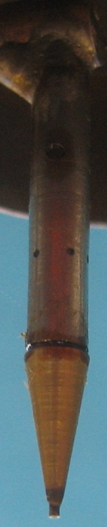
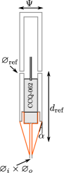
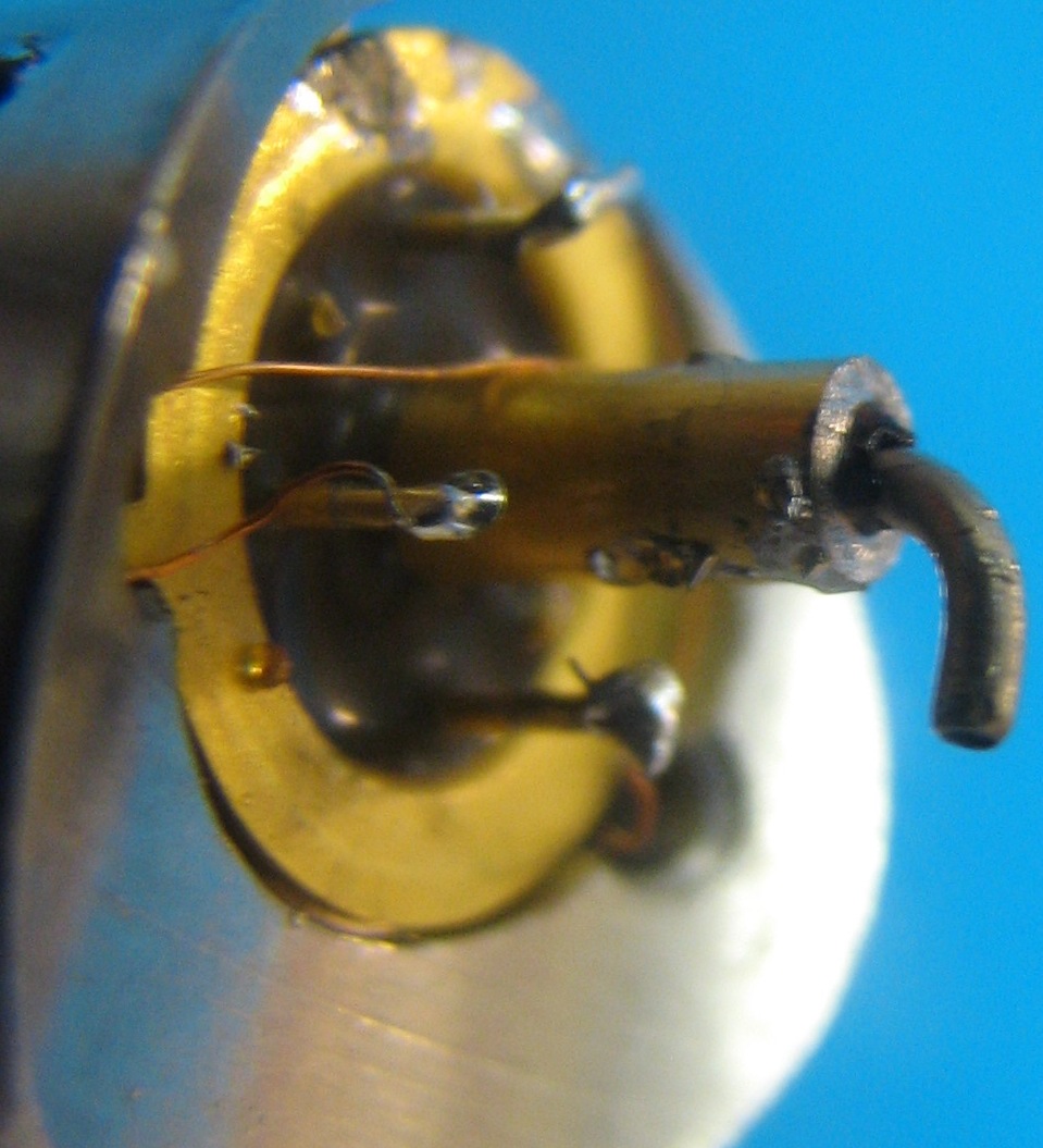
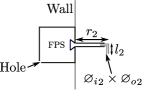
(a)

(b)

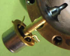
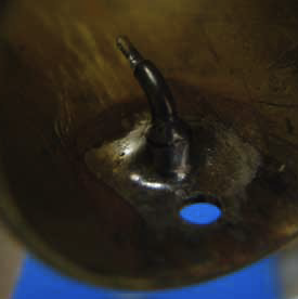
(c)

Figure 1: TSF wind tunnel probes: (a) probes ① or ③; (b) probe ②. All parts are tightly assembled. For probe ① and ③, the pressure reference is realised by holes on the outer CuNi cylinder at a distance $d_{\text{ref}}$ from the tip; for probe ②, the pressure reference is taken in a region where the flow is quiescent with a controlled leak on the back of the shell. NÉEL wind tunnel probe: (c) Probe ④ is essentially similar to probe ② except that it works as an absolute pressure probe, without hole in its shell.

Probes ①, ② and ④ have been polarized with a sinusoidal voltage. The output signal is demodulated by a lock-in amplifier. The polarisation frequency is in the range 7 — 8 kHz for probes ① and ② and in the range 10 — 20 kHz for probe ④. This modulation/demodulation technique was chosen to improve the signal to noise ratio. To make sure that no artefact bias was introduced by this method, probe ③ was polarized more simply using DC batteries. The full acquisition schematics is given on figure 2. The various properties of the probes are summarized in table 2.

Figure 2: Electronic diagram of the acquisition system for probes ① and ②. The pressure transducer is represented as a resistor bridge. The imbalance is preamplified by a low-noise preamplifier (JFET, typical noise input voltage $1~{}\mathrm{nV/\sqrt{Hz}}$). The mean value of the imbalance signal is substracted using an inductor bridge and an adjustable RC filter to compensate for the phase shift.

Table 2: Summary of the main properties of the probes used in our experiments

Probe	①	②	③	④
Transducer	Kulite	Fujikura	Kulite	Fujikura
Nose diameter [mm]	$0.4\times 0.6$	$0.6\times 0.9$	$0.4\times 0.6$	$0.6\times 0.9$
Resonance [kHz]	$\sim 2$	$\sim 2$	$\sim 2$	$<1$
Sensing	AC	AC	DC	AC

III Stagnation pressure probes used as anemometers

Following the analysis of Maurer and TabelingMaurer and Tabeling (1998), the first order term of the signal fluctuations measured by a stagnation pressure probe is linear with the local velocity fluctuations, like with Pitot tubes. However, if the turbulence intensity is too large, the second-order corrections coming from static pressure fluctuations and quadratic velocity fluctuations lead to significant bias (see appendix A for more details).

Maurer and Tabeling’s measurements were done using a stagnation pressure probe inside a turbulent Von Kármán flow. The piezoelectric probe they used was not sensitive to the DC but they could measure the turbulence intensity $\tau$ in the range 20 — 30 % in a previous measurementMaurer, Tabeling, and Zocchi (1994). According to table 5, in such conditions, the second-order corrections represent more than $\sim 20~{}\%$ of the measured signal. Additionnally, events with flow-probe angle of attack exceeding for example 15° are likely to occur at such high $\tau$, which introduces some additionnal bias on the signal interpretation. To confirm and extend Maurer and Tabeling’s result, our systematic study includes a flow with a turbulence intensity smaller than 2 %, with second-order correction smaller than 3 %. A grid flow was chosen because its turbulence is well known in classical fluids.

The calibration of the probes is done in-situ, by plotting the mean output voltage versus $\rho\left<v\right>^{2}$ where $\left<v\right>$ is the mean velocity in the channel. In the TSF wind tunnel, $\left<v\right>$ is determined by enthalpy balance across a heater. In the NÉEL wind tunnel, a Pitot tube located downstream from the probe (see figure 3) provides a measurement of the flow mean velocity.

IV Homogeneous and isotropic turbulence: the TSF grid flow

In this section, we present grid turbulence measurements in the pressurized TSF wind tunnel (see figure 3). Details about the TSF experiment have been given in previous papersRousset et al. (2008); Diribarne et al. (2009). The main dimensions are recalled in table 3. The turbulence intensity in this type of flow is typically a decade smaller than turbulent Von Kármán flows, which ensures that the fluctuating signal from the stagnation pressure probes corresponds to velocity fluctuations with less than 3 % correction. Furthermore, the pressure is maintained far above the satured vapor pressure, this ensures that no bubble can appear within the flow. However, one drawback of low turbulence intensity is that the fluctuating signal on the probe is lower, therefore the signal to noise ratio is smaller.

In this paper, we discuss two runs with different probe positions inside the test section (shown on figure 3), with mean velocities ranging from 0.4 m/s to 5 m/s and temperatures from 1.7 K and 2.6 K. The Reynolds number based on the grid mesh size $M$, $\mathrm{Re}_{M}=M\left<v\right>/\nu$ is between $10^{5}$ and $2\cdot 10^{6}$ in He I. In He II, several Reynolds numbers can be defined. Using the quantum of circulation $\kappa=h/m\simeq 9.9\times 10^{-8}~{}\mathrm{m^{2}/s}$ ($h$ is the Planck constant and $m$ is the mass of the ${}^{4}\mathrm{He}$ atom), we find $\mathrm{Re}_{\kappa}=M\left<v\right>/\kappa$ between $1.5\times 10^{4}$ and $2\times 10^{5}$.

The probe location downstream the grid is $x/M=138\pm 2$ for the first run and $x/M=121\pm 2$ for the second run. Hence we can derive the turbulence intensity and the transverse integral scale $L_{g}$ expected in He I using Comte-Bellot and Corrsin’s fits Comte-Bellot and Corrsin (1966),

$$\left<v\right>^{2}/\left<v^{\prime 2}\right>=15\left(\frac{x}{M}-\frac{x_{0}}{M}\right)^{1.2}$$ (1)

$$L_{g}/M=0.06\left(x/M-x_{0}/M\right)^{0.35}$$ (2)

where $x_{0}/M$ is the virtual origin ranging from 2 to 4.

The expected turbulence intensity in the TSF loop is therefore between 1.3 % and 1.5 % and the expected transverse integral scale $L_{g}$ lies in the range 1.2 — 1.3 mm. Alternative prefactors and exponents in equations 1 and 2 have been proposed in the literature. Using those reported by Mohamed and LaRueMohamed and LaRue (1990), we find a turbulence intensity between 0.92 % and 1.7 % for $x/M=121$ (run 2) and 0.84 % and 1.6 % for $x/M=138$ (run 1). In any cases, the turbulence intensity is small enough to safely assume that the measured signal is not polluted by static pressure fluctuations nor by large angle of attack between the flow and the probe.

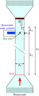
Run 1

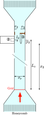
Run 2

(a)

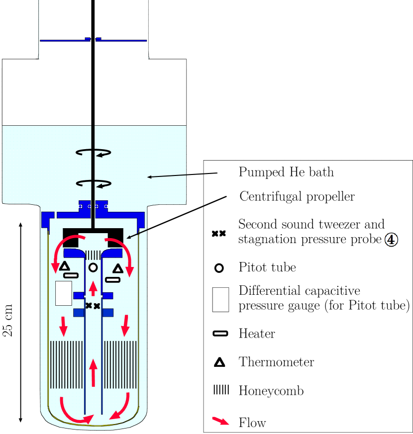
(b)

Figure 3: (a) TSF wind tunnel: Schematics of the test section and the probe locations for runs 1 and 2. For run 1, a removable cylinder can be inserted across the flow at a distance $L_{c}$ downstream the grid. It was originally designed to protect a hot-wire during the transient of the system. The stagnation pressure probe ①, located at a distance $L_{c}+L_{1}$ downstream the grid can either measure grid turbulence when the cylinder is removed or wake turbulence when the cylinder is inserted in the flow. Probe ① was not positionned on the pipe axis to avoid the wake of the hot-wire. For run 2, two stagnation pressure probes (② and ③) are available. (b) NÉEL wind tunnel: Schematics and picture of the test section and location of stagnation pressure probe ④.

Table 3: Main dimensions of the TSF wind tunnel (see figure 3 and 1 for the definition of the notations)

$\varnothing_{p}$	27.2 mm	$L_{1}$	61 mm	$l_{2}$	3 mm	$l_{3}$	9 mm
$\varnothing_{c}$	15.3 mm	$r_{1}$	8 mm	$r_{2}$	7 mm	$r_{3}$	11 mm
$L$	565 mm	${\varnothing_{i}}_{1}$	0.4 mm	${\varnothing_{i}}_{2}$	0.6 mm	${\varnothing_{i}}_{3}$	0.4 mm
$L_{c}$	479 mm	${\varnothing_{o}}_{1}$	0.6 mm	${\varnothing_{o}}_{2}$	0.9 mm	${\varnothing_{o}}_{3}$	0.6 mm
$M$	3.9 mm/mesh	$n_{M}$	7 mesh/diam	$\varnothing_{\text{ref}}$	0.5 mm	$d_{\text{ref}}$	15 mm
$\Psi$	3.5 mm	$\alpha$	15°

The velocity power spectra, $\phi(f)$, are given on figure 4, where the velocity spectral density over the time interval $[0,t_{\text{max}}]$, $\phi(f)$, is defined as

$$\phi(f)=\left|\sqrt{\frac{2}{t_{\text{max}}}}\int_{0}^{t_{\text{max}}}v^{\prime}(t)e^{-2i\pi ft}\mathrm{d}t\right|^{2}$$ (3)

The normalisation is such that

$$\int_{0}^{+\infty}\phi(f)\mathrm{d}f=\left<v^{\prime 2}\right>$$ (4)

The actual spectra are calculated using the Welch method on windows of $2^{15}$ data points. The total recording time is 7 min for most time series but we also recorded some 15 min and 30 min-long ones, with a sampling frequency of 9.77 kHz or 19.5 kHz and a high-order antialiasing filter. In He I, a Kolmogorov scaling $\phi(f)\sim f^{-5/3}$ is expected in the inertial range of the turbulent cascade. Above the corner frequency around 100 — 200 Hz, our measurements are compatible with such a scaling although the limited resolved range calls for caution. On this representation, the measurements in He II seem indistinguishable from those in He I, which suggests that the turbulence second-order statistics in the upper part of the inertial cascade are the same above and below the superfluid transition. However, this representation is not well suited for detailed comparisons because of the peaks of noise. In the following, we present more quantitative characteristics of this spectra to refine the comparison of flows in He I and He II, ie below and above the superfluid transition.

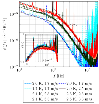
Figure 4: Grid turbulence velocity spectra acquired by probe ① for three different mean velocities both above and below the superfluid transition. The Helmholtz resonance frequency is found near 2 kHz. The solid lines are visual aids to find the corner frequency, $f_{0}$. The high-frequency lines show the -5/3 scaling. Inset: Compensated grid flow energy spectrum for various conditions both above and below the superfluid transition (see text). The value of the plateau provides an estimate for the one-dimensional Kolmogorov constant $C_{k}$ for both He I and He II grid turbulence.

We first examine the integral scale of the flow and the turbulence intensity. Both can be calculated from the spectra. The values obtained above the superfluid transition can be compared against Comte-Bellot and Corrsin’s fits for classical grid flows.

The longitudinal integral scale in the flow, $L_{l}$, can be defined as

$$L_{l}=\frac{1}{\left<v^{\prime 2}\right>}\int_{0}^{+\infty}\left<v^{\prime}(0)v^{\prime}(r)\right>\mathrm{d}r=\frac{\pi}{2}\frac{\phi(0)}{\int_{0}^{+\infty}\phi(k)\mathrm{d}k}$$ (5)

where the wavenumber $k$ and the energy spectrum in wavenumber space $\phi(k)$ are defined as,

$$\left\{\begin{array}[]{l}k=2\pi f/\left<v\right>\\ \phi(k)=\frac{\left<v\right>}{2\pi}\phi(f)\end{array}\right.$$ (6)

For an ideal flat spectrum below $k_{0}$ and a $k^{-5/3}$ scaling above $k_{0}$, we have,

$$\int_{0}^{+\infty}\phi(k)\mathrm{d}k=\frac{5}{2}\phi(0)k_{0}$$ (7)

and therefore, one can derive the observed longitudinal integral scale as $L_{l}=\frac{\left<v\right>}{10f_{0}}$ and then, assuming homogeneous isotropic turbulence, the transverse integral scale $L_{g}$ as $L_{g}=L_{l}/2$.

In our measurements, the low-frequency part of the spectrum is not flat down to a few tens of mHz. Those small fluctuations only represents some 0.1 % of the mean velocity and therefore make little change on the value of the turbulence intensity. They may come from small and slow fluctuations of the forcing mean velocity rather than from grid-generated turbulences. Therefore, it is necessary to choose a criterion to determine the corner frequency $f_{0}$. We define it as the frequency of the crossing of two power laws: one with a scaling $f^{-5/3}$ fitted on the spectrum (inertial cascade) and one with an arbitrary scaling $f^{-0.4}$ which roughly reproduces the resolved low frequency part of the spectrum. Values of corner frequencies and derived integral scales for each spectrum are summarized in table 4, including error estimates. There was more noise during run 2, which explains the larger uncertainty on $f_{0}$.

Table 4: Some integral scale measurements derived from the velocity power spectra obtained in run 1 (probe ①) and run 2 (probe ②). For comparison, Comte-Bellot and Corrsin predictions gives $L_{l}=2.6~{}\mathrm{mm}$ for run 1 and $L_{l}=2.5~{}\mathrm{mm}$ for run 2.

Run	$x$ [mm]	$\left<v\right>$ [m/s]	$f_{0}$ [Hz]	$L_{l}$ [mm]	$L_{g}$ [mm]
He I & He II identical within error bars
1	540	3.3	$140\pm 25$	$2.4\pm 0.4$	$1.2\pm 0.2$
1	540	2.5	$105\pm 25$	$2.4\pm 0.8$	$1.2\pm 0.4$
1	540	1.7	$74\pm 25$	$2.3\pm 0.9$	$1.15\pm 0.45$
He I only
2	470	4.2	$154\pm 50$	$2.7\pm 1.0$	$1.3\pm 0.5$
2	470	2.5	$98\pm 40$	$2.5\pm 1.2$	$1.25\pm 0.6$

To get the rms velocity fluctuations, or the turbulence intensity, $\tau=\sqrt{\left<v^{\prime 2}\right>}/\left<v\right>$, we calculate the area below $\phi(f)$ in a linear plot, or in practice, the area below $f\cdot\phi(f)$ in a semilog plot, to have a better estimate of the uncertainties (see inset of figure 5). We also ignored the contribution of the low-frequency increase since it is not expected to come from the turbulence cascade.

For run 1 ($x_{1}=540~{}\mathrm{mm}$), the measured turbulence intensity is found to be $\tau_{1}=(1.3\pm 0.1)~{}\%$; for run 2 ($x_{2}=470~{}\mathrm{mm}$), $\tau_{2}=(1.75\pm 0.15)~{}\%$ (see figure 5). The longitudinal integral scale are around $L_{l}=2.5~{}\mathrm{mm}$ for both runs, the error bars make it impossible to resolve the variation of $L_{l}$ between these two positions. As a first result, we find that both quantities are consistent with Comte-Bellot and Corrsin fit for classical grid flow. Besides, and more importantly, we find that both the integral scale and the turbulence intensity remain unchanged above and below the superfluid transition, within relative experimental uncertainties of 8 % for $\tau$ and 20 % for $L_{l}$.

From $\tau_{1}$ and $\tau_{2}$, we can estimate directly the turbulence dissipation rate, $\epsilon$ from the turbulent kinetic energy flux at position $x_{1}$ and $x_{2}$:

$$\epsilon\approx\left<v\right>^{3}\left|\frac{\partial\tau^{2}}{\partial x}\right|\approx\left<v\right>^{3}\frac{(\tau_{2}^{2}-\tau_{1}^{2})}{(x_{2}-x_{1})}$$ (8)

From the measured values, we can get $\partial\tau^{2}/\partial x\approx 0.0021~{}\mathrm{m^{-1}}$. This is in good agreement, with less precise alternative estimationPope (2000),

$$\epsilon\simeq 1.1\frac{\left<v^{\prime 2}\right>^{3/2}}{L_{g}}=1.1\left<v\right>^{3}\frac{\tau^{3}}{L_{g}}$$ (9)

where $1.1\tau^{3}/L_{g}$ lies in the range $0.0012\mbox{ --- }0.0045~{}\mathrm{m^{-1}}$

From $\epsilon$ and assuming isotropic and homogeneous turbulence, we can compute the turbulence micro-scale $\lambda$ in He I,

$$\epsilon=15\nu\frac{\left<v^{\prime 2}\right>}{\lambda^{2}}$$ (10)

The derived values of $\lambda$ lies in the range 70 — 230 $\mathrm{\mu m}$ and $R_{\lambda}=\lambda\sqrt{\left<v^{\prime 2}\right>}/\nu$ in the range 60 — 250. We find $R_{\lambda}\geq 100$ for most of our experimental conditions, which is consistent with the assumption of developed grid turbulence above the superfluid transition. Therefore, we expect the inertial range energy spectrum to roughly follow the Kolmogorov prediction,

$$\phi(k)=C_{k}\epsilon^{2/3}k^{-5/3}$$ (11)

On the inset of figure 4, we plot the compensated energy spectrum,

$$\psi(k)=\epsilon^{-2/3}k^{5/3}\phi(k)$$ (12)

From the value of the “plateau”, we can derive an estimate for the Kolmogorov constant, $C_{k}$, in both He I and He II. We find values in the range $C_{k}=0.3\mbox{ --- }0.4$. This is a one-dimensional Kolmogorov constant, which can be related to the three-dimensional Kolmogorov constant $C_{3d}$ assuming local isotropy,

$$C_{3d}=\frac{55}{18}C_{k}$$ (13)

We find that the three-dimensional Kolmogorov constant lies in the range $0.9\mbox{ --- }1.2$.

Previous normal fluid grid flow experimentsComte-Bellot and Corrsin (1971); Gad-el-Hak and Corrsin (1974); Gibson and Schwarz (1963); Schedvin, Stegen, and Gibson (1974) have reported measured values of the Kolmogorov constant scatteredSreenivasan (1995) around $C_{3d}=1.5$, in the window $C_{3d}=1.0\mbox{ --- }1.74$ (ie. $C_{k}=0.33\mbox{ --- }0.57$). The value that we find is close to the smaller values reported in the literature. Our emphasis will not be on the actual value that we have measured. Indeed, the latter can be affected by systematic errors, such as systematic bias on the probe calibration. However, it is quite remarkable that our measure of the Kolmogorov constant in He II down to 2.0 K coincides with the value measured in He I within 30 % relative error margin.

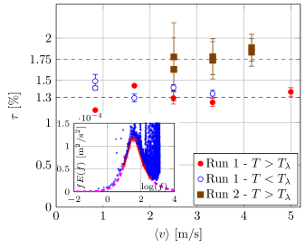
Figure 5: Turbulence intensity $\tau$ measured for the two grid flow runs in the TSF wind tunnel, for various velocities and temperatures, computed using the integral of the energy spectrum. Inset: Estimation of the envelope of the energy spectrum. The area below the envelope is the energy of the velocity fluctuations. The dots are experimental data points, the solid line is the estimated envelope below the spectrum and the dashed line is the extrapolated spectrum (flat spectrum in the low frequency limit and $f^{-5/3}$ scaling in the high frequency limit). The energy from the low frequency $f^{-0.4}$ increase is not taken in the turbulent energy estimate. However, this makes a relative difference smaller than a few percents in the final estimate.

V High turbulence intensity flows

We report two sets of high turbulence intensity flows: measurements done in the TSF wind tunnel in the near wake of a cylinder (see schematics of run 1 on figure 3-a) and measurements done in the NÉEL wind tunnel, sketched on figure 3-c and described in more details elsewhereRoche et al. (2007). The main advantage of such flows is a better signal-to-noise ratio. However, the turbulence is less homogeneous and less isotropic, especially in the near wake flow.

V.1 Near wake flow

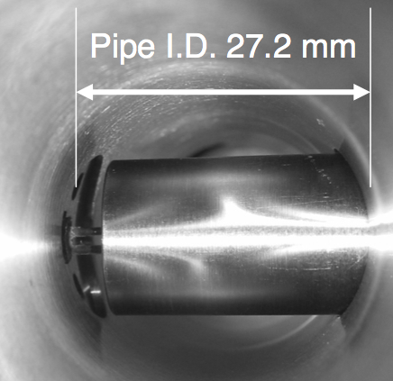
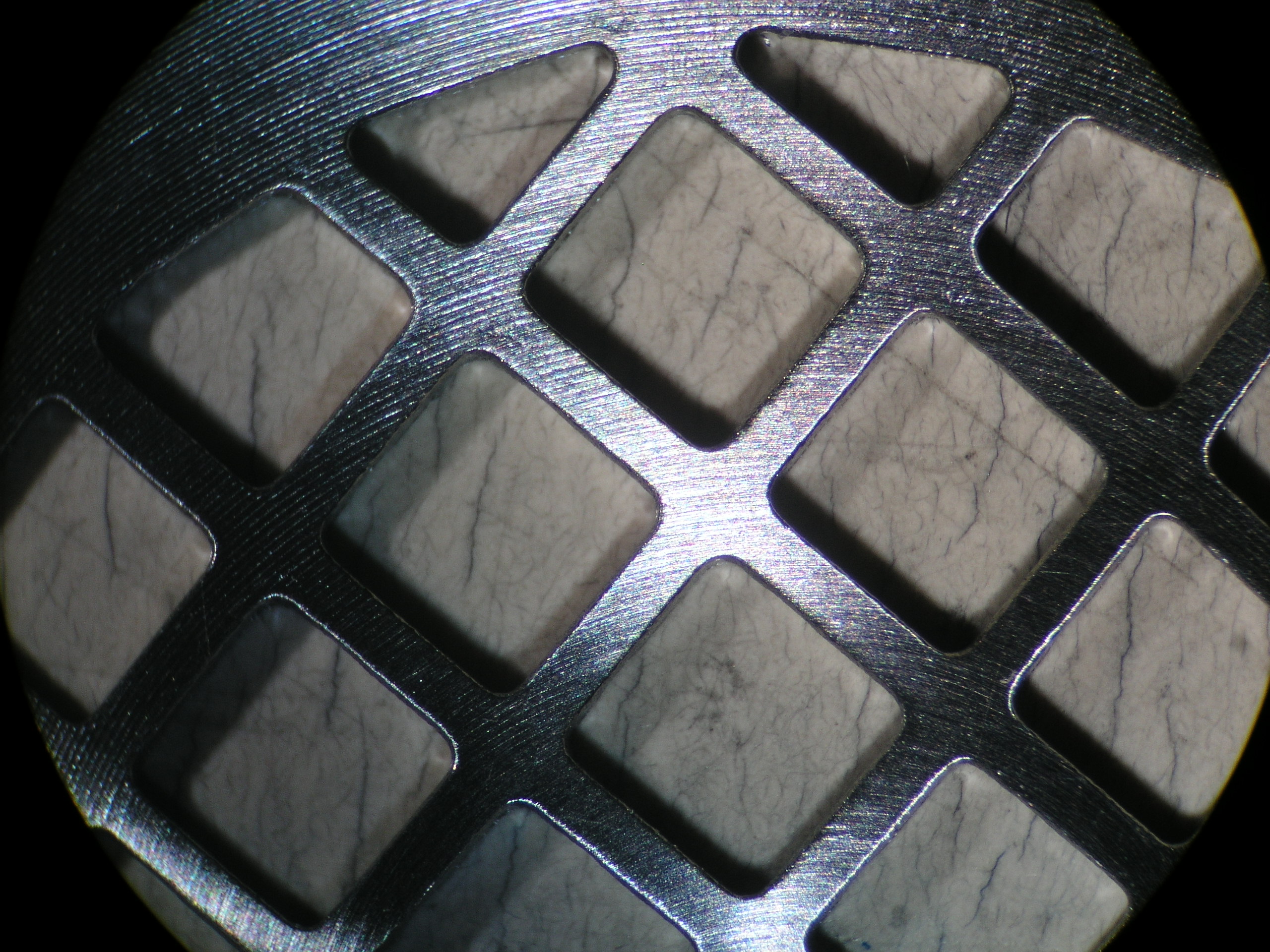
Figure 6: Left: picture of the removable cylinder in the TSF wind tunnel. The angle between the probe and the axis of the pipe is 17°. Right: picture of the grid.

The cylinder used in the TSF wind tunnel was originally designed to protect a hot-wire during the filling of the cryogenic loop, in particular to avoid droplets from colliding with the wire. Therefore, the dimensions are not designed to produce fully developed wake turbulence. As shown on table 3, the wake cylinder diameter $\varnothing_{c}$ is 15.3 mm for a pipe diameter $\varnothing_{p}$ of 27.2 mm, leading to a significant wall confinement. Besides, the cylinder length is slightly smaller than the pipe diameter as shown on figure 6. The dimentionless distance between the cylinder axis and the sensor, $L_{1}/\varnothing_{c}$ is $4.0\pm 0.3$. The cylinder Reynolds number $\varnothing_{c}\left<v\right>/\nu$ falls in the range $3\times 10^{5}$ — $2\times 10^{6}$, where $\left<v\right>$ is estimated upstream (or downstream) from the cylinder, and not on the constriction where $\left<v\right>$ is larger. In a less confined geometry, the Strouhal number,

$$\mathrm{St}=\frac{f_{v}\varnothing_{c}}{\left<v\right>}$$ (14)

where $f_{v}$ is the frequency of vortex shedding, is undefined at such Re in classical fluidsLienhard (1966). Finally, we point that this flow geometry can lead to large angle of attack on the probe.

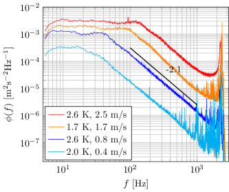
Figure 7: Velocity spectra in the near wake of a cylinder in the TSF wind tunnel both above and below the superfluid transition with mean velocity increasing from bottom to top. The high frequency peak near 2 kHz is the sensor Helmholtz frequency.

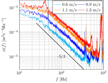
Figure 8: Velocity spectra for $T=1.55~{}\mathrm{K}$ in the NÉEL wind tunnel for four mean velocities below the superfluid transition. The low frequency corners give an estimate of the longitudinal integral scale $L_{g}=2~{}\mathrm{cm}$.

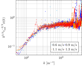
Figure 9: Same data as figure 8 plotted in a compensated fashion (see text).

Figure 7 shows spectra in the near wake of the cylinder in both He I and He II. No sharp Strouhal peak is visible, either above or below the superfluid transition. The slope is steeper than -5/3. One possible explanation is that the spectral distribution of energy right after the obstacle is concentrated at the largest scales and by the time the probe is reached, it has not developped yet into the Kolmogorov cascade. As another possible explanation, we also point out that velocity spectra in strongly inhomogeneous classical flows, in particular near a stable vortex, are knownSimand, Chillà, and Pinton (2000) to scale like $f^{-\alpha}$, with $\alpha$ in the range 1.65 — 2.50. In any case, our result shows that the indistinguishability between He I and He II does not require an equilibrium state in the sense of Kolmogorov.

V.2 Chunk turbulence

The NÉEL wind tunnel is placed in a saturated liquid helium bath (see figure 3-c). The temperature is controlled mainly by the bath pressure and fine-tuned by a temperature regulator. The data discussed here are obtained at $T=1.55~{}\mathrm{K}$, which corresponds to a superfluid fraction $\rho_{s}/\rho\approx 86~{}\%$. Above the superfluid transition, bubbles are likely to appear in saturated baths. Therefore we only report measurements below the superfluid transition, where the absence of thermal gradients prevents the forming of bubbles. The turbulence is generated by a continuously powered centrifugal pump and probed by stagnation pressure probe ④ and a local quantum vortex lines density probes in a 23 mm-diameter, 250 mm-long brass pipe, located upstream from the pump. The analysis of the quantum vortex lines density results are discussed in a previous paperRoche et al. (2007); Roche and Barenghi (2008). The useful range of velocity is 0.25 — 1.3 m/s. The typical turbulence intensity is roughly constant in this range of parameters. Its value is $(18\pm 1)~{}\%$ if we choose to remove the energy that comes from the low-frequency variation of the mean velocity, like we did in the previous parts; or in the range 25 % — 35 %, if we choose to keep all the measured energy, like was done in the previous paperRoche et al. (2007). The superfluid Reynolds number $\mathrm{Re}_{\kappa}=\varnothing V/\kappa$ falls in the range $6\times 10^{4}$ — $3\times 10^{5}$.

Figure 8 shows spectra obtained in the NÉEL wind tunnel in He II. They show one decade of $f^{-\alpha}$ scaling, with $\alpha=1.55\mbox{ --- }1.69$. This is compatible with a Kolmogorov -5/3 turbulent cascade with a relative experimental error bar of less than 7 % on the exponent. The compensated spectra are shown on figure 9 using $\epsilon_{\text{est}}=\left<v^{\prime 2}\right>^{3/2}/L_{g}$ and $L_{g}=1~{}\mathrm{cm}$. From the value of the “plateau”, we find a one-dimensional Kolmogorov constant around $0.5$. Although the “chunky” aspect of the flow prevents to speculate on its value, we note that it is in good agreement with values in a classical flows.

VI Conclusions & perspectives

We have done systematic superfluid velocity measurements in three different highly turbulent flows. The upper inertial range of the turbulent cascade was resolved with various anemometers based on stagnation pressure probes. We found that the second order statistics of the superfluid velocity fluctuations does not seem to differ from those of classical turbulence down to the precision of our measurements.

It is worth pointing that non conventional velocity statistics have been recently reported in superfluid flows, both in an experimentalPaoletti et al. (2008) and a numericalWhite et al. (2010) study. These studies where conducted at a much lower effective Reynolds number and the probing of the flow velocity was done at a scale where quantum effects are prevalent. In the present work, the characteristic length scale of quantum effect is much lower than the probe resolution. For example, in the NÉEL flow, the typical distance between two neighbouring quantum vorticies is a few micronsRoche and Barenghi (2008), to be compared with the probe resolution of 1 mm typically.

To go further into the physics of quantum turbulence, it would be necessary to resolve the small scales of a high-Reynolds number flow. To do this at given Reynolds number, one should either increase the cut-off scale by scaling up the experiment or decrease the size of the probe. However, it is delicate to reduce the size of stagnation pressure probes below-say-$200~{}\mathrm{\mu m}$. One alternative is to design new types of probes — for example, adapting cantilever-based anemometersBarth et al. (2005) to low temperatures.

Appendix A Derivation of the stagnation pressure signal

We consider the total pressure $U(t)$ measured by a stagnation pressure probe in a classical incompressible fluid,

$$U(t)=\frac{1}{2}\rho v(t)^{2}+P(t)$$ (15)

where $\rho$ is the density of the fluid, $v(t)$ the local velocity and $P(t)$ the local static pressure. Equation 15 can be rewritten using Reynolds decomposition $v(t)=\left<v\right>+v^{\prime}(t)$ and $P(t)=\left<P\right>+P^{\prime}(t)$,

$$U(t)=\frac{1}{2}\rho\left<v\right>^{2}+\left<P\right>+\rho\left<v\right>v^{\prime}(t)+P^{\prime}(t)+\frac{1}{2}\rho v^{\prime}(t)^{2}$$ (16)

We recall the definition of the turbulence intensity $\tau$,

$$\tau=\frac{\sqrt{\left<v^{\prime 2}\right>}}{\left<v\right>}$$ (17)

The typical magnitude of the static pressure fluctuation $P^{\prime}$ can be estimated for isotropic and homogeneous turbulenceUberoi (1953); Batchelor (1951); Schumann and Patterson (1978),

$$\frac{\sqrt{\left<P^{\prime 2}\right>}}{\frac{1}{2}\rho\left<v^{\prime 2}\right>}\approx 1.4$$ (18)

Therefore, the terms of equation 16 can be divided in orders of $\tau$,

$$\left\{\begin{array}[]{lclcl}U_{0}&=&\frac{1}{2}\rho\left<v\right>^{2}+\left<P\right>&=&\mathcal{O}(1)\\ U_{1}(t)&=&\rho\left<v\right>v^{\prime}(t)&=&\mathcal{O}(\tau)\\ U_{2}(t)&=&P^{\prime}(t)+\frac{1}{2}\rho v^{\prime}(t)^{2}&=&\mathcal{O}(\tau^{2})\end{array}\right.$$ (19)

$U_{0}$ is a constant offset, used only for calibrating the probe, $U_{1}(t)$ is the signal of interest and $U_{2}(t)$ is the second order corrective term, considered as a spurious signal for stagnation pressure probes. The relative weight of $U_{2}$ versus $U_{1}$ can be estimated versus the turbulent intensity $\tau$,

$$\begin{array}[]{rcc}U_{1}(t)&=&\rho\left<v\right>v^{\prime}(t)\sim\rho\left<v\right>^{2}\tau\\ U_{2}(t)&=&\left\{\begin{array}[]{rcl}P^{\prime}(t)&\sim&0.7\rho\left<v\right>^{2}\tau^{2}\\ \frac{1}{2}\rho v^{\prime}(t)^{2}&\sim&0.5\rho\left<v\right>^{2}\tau^{2}\end{array}\right.\end{array}$$ (20)

Some values are given in table 5. We can see that for turbulence intensity larger than 20 %, like those obtained in Von Kármán cells, and in wake or “chunk” flows, almost 30 % of the measured signal comes from second order correction terms. However, for turbulence intensities of grid flows, less than 2 % in our case, more than 96 % of the measured signal comes from the linear velocity term.

Table 5: Typical relative weight of each term contributing to the signal measured by a stagnation pressure probe for various turbulence intensity $\tau$ using the estimate (20)

$\tau$	$\rho\left<v\right>v^{\prime}(t)$	$P^{\prime}(t)$	$\frac{1}{2}\rho v^{\prime}(t)^{2}$
1 %	98.8 %	0.7 %	0.5 %
2 %	97.6 %	1.4 %	1 %
10 %	89.2 %	6.3 %	4.5 %
20 %	80.6 %	11.3 %	8.1 %
30 %	73.5 %	15.5 %	11.0 %

REFERENCES

REFERENCES

- Landau and Lifshitz (1987) L. Landau and E. Lifshitz, Fluid Mechanics, 2nd ed., Course of Theoretical Physics, Vol. 6 (1987).
- Castaing et al. (1994) B. Castaing, B. Chabaud, B. Hébral, A. Naert, and J. Peinke, “Turbulence at helium temperature: velocity measurements,” Physica B 194-196, 697–698 (1994).
- Zocchi et al. (1994) G. Zocchi, P. Tabeling, J. Maurer, and H. Willaime, “Measurement of the scaling of the dissipation at high reynolds numbers,” Phys. Rev. E 50, 3693 (1994).
- Chanal et al. (2000) O. Chanal, B. Chabaud, B. Castaing, and B. Hébral, “Intermittency in a turbulent low temperature gaseous helium jet,” Eur. Phys. J. B 17, 309–317 (2000).
- Pietropinto et al. (2003) S. Pietropinto, C. Poulain, C. Baudet, B. Castaing, B. Chabaud, Y. Gagne, B. Hébral, Y. Ladam, P. Lebrun, O. Pirotte, and P. Roche, “Superconducting instrumentation for high reynolds turbulence experiments with low temperature gaseous helium,” Physica C 386, 512–516 (2003).
- Holmes and Sciver (1992) D. S. Holmes and S. V. Sciver, “Attenuation of second sound in bulk flowing He II,” J. Low Temp. Phys. 87, 73–93 (1992).
- Smith et al. (1993) M. R. Smith, R. J. Donnelly, N. Goldenfeld, and W. F. Vinen, “Decay of vorticity in homogeneous turbulence,” Phys. Rev. Lett. 71, 2583 (1993).
- Stalp and Niemela (2002) S. R. Stalp and J. J. Niemela, “Dissipation of grid turbulence in helium II,” Phys. fluids 14, 1377 (2002).
- Skrbek, Gordeev, and Soukup (2003) L. Skrbek, A. Gordeev, and F. Soukup, “Decay of counterflow He II turbulence in a finite channel: Possibility of missing links between classical and quantum turbulence,” Phys. Rev. E 67, 047302 (2003).
- Roche et al. (2007) P.-E. Roche, P. Diribarne, T. Didelot, O. Français, L. Rousseau, and H. Willaime, “Vortex density spectrum of quantum turbulence,” EPL 77, 66002 (2007).
- Maurer and Tabeling (1998) J. Maurer and P. Tabeling, “Local investigation of superfluid turbulence,” EPL 43, 29–34 (1998).
- Note (1) The confirmation previously cited by Roche, et al.Roche et al. (2007) is presented in the present paper.
- Merahi, Sagaut, and Abidat (2006) L. Merahi, P. Sagaut, and M. Abidat, “A closed differential model for large-scale motion in HVBK fluids,” EPL 75, 757–763 (2006).
- Roche, Barenghi, and Lévêque (2009) P.-E. Roche, C. Barenghi, and E. Lévêque, “Quantum turbulence at finite temperature: The two-fluids cascade,” EPL 87, 54006 (2009).
- Nore, Abid, and Brachet (1997) C. Nore, M. Abid, and M. Brachet, “Decaying Kolmogorov turbulence in a model of superflow,” Phys. fluids 9, 2644 (1997).
- Araki, Tsubota, and Nemirovskii (2002) T. Araki, M. Tsubota, and S. K. Nemirovskii, “Energy spectrum of superfluid turbulence with no normal-fluid component,” Phys. Rev. Lett. 89, 145301 (2002).
- Kobayashi and Tsubota (2005) M. Kobayashi and M. Tsubota, “Kolmogorov spectrum of superfluid turbulence: Numerical analysis of the gross-pitaevskii equation with a small-scale dissipation,” Phys. Rev. Lett. 94, 065302 (2005).
- Vinen and Niemela (2002) W. F. Vinen and J. J. Niemela, “Quantum turbulence,” J. Low Temp. Phys. 128, 167–231 (2002).
- Haruyama, Kimura, and Nakamoto (1998) T. Haruyama, N. Kimura, and T. Nakamoto, “FPS51B - a small piezo-resistive silicon pressure sensor for use in superfluid helium,” in 17th International Cryogenic Engineering Conference, ICEC17 (1998).
- Maeda et al. (2004) M. Maeda, A. Sato, M. Yuyama, M. Kosuge, F. Matsumoto, and H. Nagai, “Characteristics of a silicon pressure sensor in superfluid helium pressurized up to 1.5 MPa,” Cryogenics 44, 217–222 (2004).
- Maurer, Tabeling, and Zocchi (1994) J. Maurer, P. Tabeling, and G. Zocchi, “Statistics of turbulence between 2 counterrotating disks in low-temperature helium gas,” EPL 26, 31–36 (1994).
- Rousset et al. (2008) B. Rousset, C. Baudet, M. B. Mardion, B. Castaing, D. Communal, F. Daviaud, P. Diribarne, B. Dubrulle, A. Forgeas, Y. Gagne, A. Girard, B. Hébral, P.-E. Roche, P. Roussel, and P. Thibault, “Tsf experiment for comparison of high reynolds number turbulence in both He I and He II: First results,” in Advances in cryogenic engineering, CEC ICMC, AIP Conference Proceedings, Vol. 53 (Chattanooga France, 2008) p. 633.
- Diribarne et al. (2009) P. Diribarne, J. Salort, C. Baudet, B. Belier, B. Castaing, L. Chevillard, F. Daviaud, S. David, B. Dubrulle, Y. Gagne, A. Girard, B. Rousset, P. Tabeling, P. Thibault, H. Willaime, and P.-E. Roche, “TSF experiment for comparison of high reynolds number turbulence in He I and He II: first results,” in Advances in Turbulence XII, ETC12, edited by B. Eckhardt (2009) p. 701.
- Comte-Bellot and Corrsin (1966) G. Comte-Bellot and S. Corrsin, “The use of a contraction to improve the isotropy of grid-generated turbulence,” J. Fluid Mech. 25, 657–682 (1966).
- Mohamed and LaRue (1990) M. S. Mohamed and J. C. LaRue, “The decay power law in grid-generated turbulence,” J. Fluid Mech. 219, 195–214 (1990).
- Pope (2000) S. B. Pope, Turbulent flows (Cambridge University Press, 2000).
- Comte-Bellot and Corrsin (1971) G. Comte-Bellot and S. Corrsin, “Simple eulerian time correlation of full- and narrow-band velocity signals in grid-generated ’isotropic’ turbulence,” J. Fluid Mech. 48, 273–337 (1971).
- Gad-el-Hak and Corrsin (1974) M. Gad-el-Hak and S. Corrsin, “Measurements of the nearly isotropic turbulence behind a uniform jet grid,” J. Fluid Mech. 62, 115–143 (1974).
- Gibson and Schwarz (1963) C. Gibson and W. Schwarz, “The universal equilibrium spectra of turbulent velocity and scalar fields,” J. Fluid Mech. 16, 365–384 (1963).
- Schedvin, Stegen, and Gibson (1974) J. Schedvin, G. Stegen, and C. Gibson, “Universal similarity at high grid reynolds numbers,” J. Fluid Mech. 65, 561–579 (1974).
- Sreenivasan (1995) K. R. Sreenivasan, “On the universality of the Kolmogorov constant,” Phys. fluids 7, 2778 (1995).
- Lienhard (1966) J. H. Lienhard, “Synopsis of lift, drag, and vortex frequency data for rigid circular cylinders,” Research Division Bulletin, Washington State University 300 (1966).
- Simand, Chillà, and Pinton (2000) C. Simand, F. Chillà, and J.-F. Pinton, “Inhomogeneous turbulence in the vicinity of a large-scale coherent vortex,” EPL 49, 336–342 (2000).
- Roche and Barenghi (2008) P.-E. Roche and C. Barenghi, “Vortex spectrum in superfluid turbulence: Interpretation of a recent experiment,” EPL 81, 36002 (2008).
- Paoletti et al. (2008) M. Paoletti, M. E. Fisher, K. Sreenivasan, and D. Lathrop, “Velocity statistics distinguish quantum turbulence from classical turbulence,” Phys. Rev. Lett. 101, 154501 (2008).
- White et al. (2010) A. White, C. Barenghi, N. Proukakis, A. Youd, and D. Wacks, “Nonclassical velocity statistics in a turbulent atomic bose-einstein condensate,” Phys. Rev. Lett. 104, 075301 (2010).
- Barth et al. (2005) S. Barth, H. Koch, A. Kittel, J. Peinke, J. Burgold, and H. Wurmus, “Laser-cantilever anemometer: A new high-resolution sensor for air and liquid flows,” Rev. Sci. Instrum. 76, 075110 (2005).
- Uberoi (1953) M. Uberoi, “Quadruple velocity correlations and pressure fluctuations in isotropic turbulence,” J. Aero. Sci 20, 197–204 (1953).
- Batchelor (1951) G. Batchelor, “Pressure fluctuations in isotropic turbulence,” Proc. Camb. Phil. Soc. 47, 359–374 (1951).
- Schumann and Patterson (1978) U. Schumann and G. Patterson, “Numerical study of pressure and velocity fluctuations in nearly isotropic turbulence,” J. Fluid Mech. 88, 685–709 (1978).