The correlation function of galaxy clusters and detection of baryon acoustic oscillations

Abstract

We calculate the correlation function of 13 904 galaxy clusters of $z\leq 0.4$ selected from the cluster catalog of Wen, Han & Liu. The correlation function can be fitted with a power-law model $\xi(r)=\left(r/R_{0}\right)^{-\gamma}$ on the scales of $10~{}h^{-1}{\rm Mpc}\leq r\leq 50~{}h^{-1}{\rm Mpc}$, with a larger correlation length of $R_{0}=18.84\pm 0.27~{}h^{-1}{\rm Mpc}$ for clusters with a richness of $R\geq 15$ and a smaller length of $R_{0}=16.15\pm 0.13~{}h^{-1}{\rm Mpc}$ for clusters with a richness of $R\geq 5$. The power law index of $\gamma=2.1$ is found to be almost the same for all cluster subsamples. A pronounced baryon acoustic oscillations (BAO) peak is detected at $r\sim 110~{}h^{-1}{\rm Mpc}$ with a significance of $\sim 1.9\sigma$. By analyzing the correlation function in the range of $20~{}h^{-1}{\rm Mpc}\leq r\leq 200~{}h^{-1}{\rm Mpc}$, we find the constraints on distance parameters are $D_{v}(0.276)=1077\pm 55(1\sigma){~{}\rm Mpc}$ and $h=0.73\pm 0.039(1\sigma)$, which are consistent with the WMAP 7-year cosmology. However, the BAO signal from the cluster sample is stronger than expected and leads to a rather low matter density $\Omega_{m}h^{2}=0.093\pm 0.0077(1\sigma)$, which deviates from the WMAP 7-year result by more than $3\sigma$. The correlation function of the GMBCG cluster sample is also calculated and our detection of the BAO feature is confirmed.

1. Introduction

One of the most important tasks of modern redshift surveys (e.g. York et al., 2000; Colless et al., 2001) is to reveal the large-scale structure of the universe. Observations have shown that galaxies are not uniformly distributed in the universe (Hawkins et al., 2003; Zehavi et al., 2004). They not only cluster on the scales of Mpc (e.g. Abell et al., 1989; Wen et al., 2009) but also are embedded in large-scale diverse structures which have scales of tens of Mpc, exhibited as filaments, walls and voids (Geller & Huchra, 1989; Gott et al., 2005). Large-scale baryon fluctuations bear the imprint of acoustic oscillations in the tightly coupled baryon-photon fluid prior to the epoch of recombination (Peebles & Yu, 1970; Sunyaev & Zeldovich, 1970).

To reveal the large-scale baryon acoustic oscillation (BAO) feature in the universe (Eisenstein, 2002, 2005; Martínez, 2009), a large sample of tracers in a huge volume of the order $1~{}h^{-3}{\rm Gpc^{3}}$ need to be observed. Galaxies, especially the Luminous Red Galaxies (LRGs), are the most popular tracers used. The Sloan Digital Sky Survey (SDSS, York et al., 2000) has observed the spectra for an unprecedently large sample of galaxies. Using the LRG sample from the SDSS Data Release 3 (DR3), Eisenstein et al. (2005) firstly detected the BAO signal ($\sim 3.4\sigma$) at a scale of $r\sim 100~{}h^{-1}{\rm Mpc}$ in the correlation functions of LRGs, which has recently been updated by Percival et al. (2010) and Kazin et al. (2010) using new LRG samples from the SDSS DR7. Blake et al. (2011a) and Beutler et al. (2011) detected the BAO features using the data from the WiggleZ and 6dF galaxy surveys, respectively.

Being the largest gravitationally bound systems in the universe, galaxy clusters are formed from more massive halos than galaxies. They are more strongly correlated in space than galaxies. Clusters can be identified from photometric survey data by visual inspection (Abell, 1958; Abell et al., 1989) or automatic cluster-finding algorithms if the redshifts of galaxies are available (Gal et al., 2003; Lopes et al., 2004). Because of lack of spectroscopic data of galaxies, galaxy clusters previously identified in limited volumes of the universe are hard to be used for the BAO detection. Miller et al. (2001) showed the power spectrum with a possible BAO feature from the redshift data of the Abell/ACO clusters, Infrared Astronomical Satellite (IRAS) point sources and the Automated Plate Measurement (APM) clusters. Using the large sample of galaxy redshift data obtained from spectral observations or estimated from photometric data of SDSS (York et al., 2000), a large number of galaxy clusters have been identified (Koester et al., 2007a, b; Wen et al., 2009) in the vast volume up to redshift $z\sim 0.6$. They can be used to trace the large scale structure and constrain cosmological parameters, e.g. the mass fluctuation on the scale of $8~{}h^{-1}{\rm Mpc}$, $\sigma_{8}$ (Wen et al., 2010). Estrada et al. (2009) detected the BAO signature ($1.4\sigma\sim 1.7\sigma$) from the cluster correlation function using the maxBCG cluster sample (Koester et al., 2007a, b). Hütsi (2010) also found the BAO feature ($\sim 2.2\sigma$) in the redshift-space power spectrum of the maxBCG cluster sample.

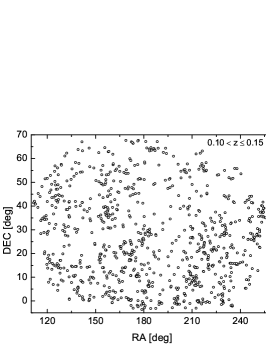
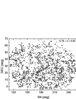
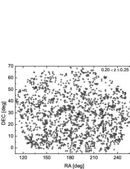
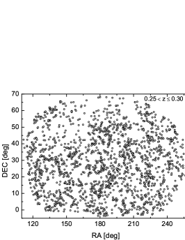
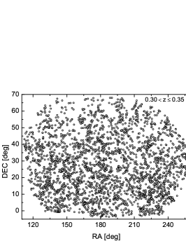
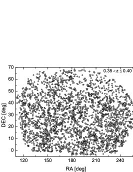
Figure 1.— Sky distribution of galaxy clusters in our sample shown in 6 redshift bins. We discard clusters in the four separated stripes to eliminate the boundary effect in calculation of the correlation function.

In this paper, we work on the 2-point correlation function for clusters selected from Wen et al. (2009) to show the power-law clustering on small scales and the BAO feature on large scales. We describe our cluster sample in Section 2. In Section 3 we present the correlation functions. The power-law clustering of clusters is studied for different richnesses of clusters. In Section 4, we analyze the BAO feature and its cosmological implication. We verify our BAO detection using the correlation function of the GMBCG clusters cataloged by Hao et al. (2010). Conclusions are presented in Section 5.

Throughout this paper, we adopt a flat $\Lambda$CDM cosmology, with $h=0.71$, $\Omega_{m}=0.27$, $\Omega_{\Lambda}=0.73$, $\sigma_{8}=0.8$, where $h\equiv H_{0}/100{\rm kms^{-1}Mpc^{-1}}$.

2. Galaxy Cluster Sample

Using the photometric data of the SDSS DR6, Wen et al. (2009) identified 39 668 galaxy clusters in the redshift of $0.05<z<0.60$. This is the largest cluster sample before the GMBCG clusters were cataloged by Hao et al. (2010). All clusters in Wen et al. (2009) contain more than eight luminous ($M_{r}\leq-21$) member galaxies. Due to lack of spectroscopic redshifts for distant and faint galaxies, photometric redshifts of galaxies (Csabai et al., 2003) were used in the cluster-finding algorithm. The median photometric redshift of member galaxies is adopted to be the redshift of a cluster. By comparing the estimated redshifts of 13 620 clusters with the spectroscopic redshifts of the brightest cluster galaxies (BCGs), Wen et al. (2009) found that the distribution of cluster redshifts statistically have an offset of less than 0.002 or 0.003 from the true value and the standard deviation around 0.02. Their Monte Carlo simulations show that the false detection rate is about 5%. Massive clusters of $M_{200}>2\times 10^{14}{\rm M_{\odot}}$ have a high completeness of more than 90% up to $z=0.42$.

Although photometric redshifts of galaxies can be used to identify clusters, the redshift uncertainties of clusters can smear out the radial distribution in the large-scale structures. It has been shown that the large uncertainty of $\sigma_{z}\sim 0.01$ is obviously the obstacle for detection of BAO signature (Blake & Bridle, 2005; Zhan et al., 2008). Estrada et al. (2009) used the 13 823 maxBCG clusters with redshift uncertainty of $\sigma_{z}\sim 0.015$ and found only weak evidence ($1.4\sigma-1.7\sigma$) for the BAO peak from the 3D correlation function.

Figure 2.— Redshift distribution of 13 904 clusters in our sample.

We calculate the correlation function of the selected clusters from Wen et al. (2009). A cluster is selected only if the spectroscopic redshift of at least one of member galaxies is available from the SDSS DR8. To eliminate selection effect of the boundary on the correlation function, we discard the clusters in the four small separated stripes in the SDSS sky. Because the clusters of $z\leq 0.4$ construct a relative complete sample (Wen et al., 2009), we discard all clusters of $z>0.4$. There are 19 828 clusters of $z\leq 0.40$ in total. Among them, 11 103 clusters have their BCG spectroscopically observed, so that we adopt the redshift of the BCG as the cluster redshift; 2 801 clusters have at least one of the member galaxies (not BCG) spectroscopically observed, for which we adopt the redshift of the galaxy or the mean of spectroscopic galaxy redshifts as the cluster redshift. These 13 904 clusters in the sky area of $\sim 7\,100$ square degree shown in Figure 1 are used for calculation of the correlation fuction. These are the two-third of all clusters randomly observed for spectroscopical redshifts. The redshift distribution of the cluster sample is shown in Figure 2. The mean redshift of the whole sample is $z_{m}=0.276$.

3. Correlation function of clusters

Two kinds of statistics are often used to describe the large-scale clustering and BAO features. One is the 2-point correlation function which describes the probability to find another object within a given radius (Peebles, 1980). The other is the power spectrum of object distribution, which is the Fourier transform of the correlation function. Both depict the same statistical distribution properties but in different forms. In this paper, we calculate the 2-point correlation function $\xi(r)$ for galaxy clusters using the Landy-Szalay estimator (Landy & Szalay, 1993),

$$\xi(r)=\left[DD(r)\frac{N_{RR}}{N_{DD}}-2\;DR(r)\frac{N_{RR}}{N_{DR}}+RR(r)\right]/RR(r),$$ (1)

which compares the cluster pair counts with the simulated random points. Here $DD(r)$ stands for the number of cluster pairs, i.e. data-data pairs, within a separation annulus of $r\pm\Delta r/2$, $DR(r)$ is the number of data-random pairs, and $RR(r)$ is the number of random-random pairs. $N_{DD}$, $N_{DR}$ and $N_{RR}$ are the normalization factors for the three pair counts. To minimize the calculation noise from the random data, we simulate the random sample 16 times larger than the data sample, which covers the same sky area (Figure 1) and has the same redshift distribution (Figure 2).

We use the jackknife method to estimate the error covariance for the correlation function. We divide the sky area into 32 disjoint sky sub-areas, each with approximately the same area as the others. We define a subsample of clusters by removing the clusters in only one sub-area. Correlation functions are calculated 32 times for 32 different subsamples. The uncertainties of $\xi(r)$ at different $r$ are interdependent. The covariance matrix is then constructed as follows:

$$C_{ij}=\frac{N-1}{N}\sum_{k=1}^{N}\left(\xi^{k}_{i}-\overline{\xi}_{i}\right)\left(\xi^{k}_{j}-\overline{\xi}_{j}\right),$$ (2)

where $N=32$ is the number of subsample, $\xi^{k}_{i}$ represents the correlation function value of the $k^{th}$ subsample at the $i^{th}$ bin of $r$ values, and $\overline{\xi}_{i}$ is the mean value of the all 32 subsamples at the $i^{th}$ bin. The error bars of $\xi(r)$ are given by the diagonal elements as $\sigma_{i}=\sqrt{C_{ii}}$.

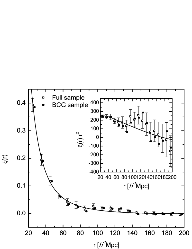
Figure 3.— Correlation function of 13 904 clusters (squares) and 11 103 clusters with known redshifts of BCGs (dots, shifted to right by $2~{}h^{-1}{\rm Mpc}$ for plotting clarity). The solid line is the best-fit $\Lambda$CDM model without acoustic feature for the full sample. To show the large-scale BAO feature more clearly, we plot $\xi(r)r^{2}$ in the inset.

Using the 3-D spatial distribution of 13 904 clusters with spectroscopic redshifts, we calculate the correlation function $\xi(r)$ and the uncertainty in 18 bins from $20~{}h^{-1}{\rm Mpc}$ to $200~{}h^{-1}{\rm Mpc}$ (see Figure 3). The correlation function on small scales follows a power law, and the BAO feature appears at $r\sim 110~{}h^{-1}{\rm Mpc}$. For comparison, we calculate the correlation function for 11 103 clusters which have the redshift of the BCG spectroscopically observed. As shown in Figure 3, the correlation function of the BCG sample is consistent with the full sample of 13 904 clusters.

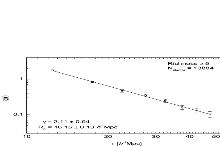
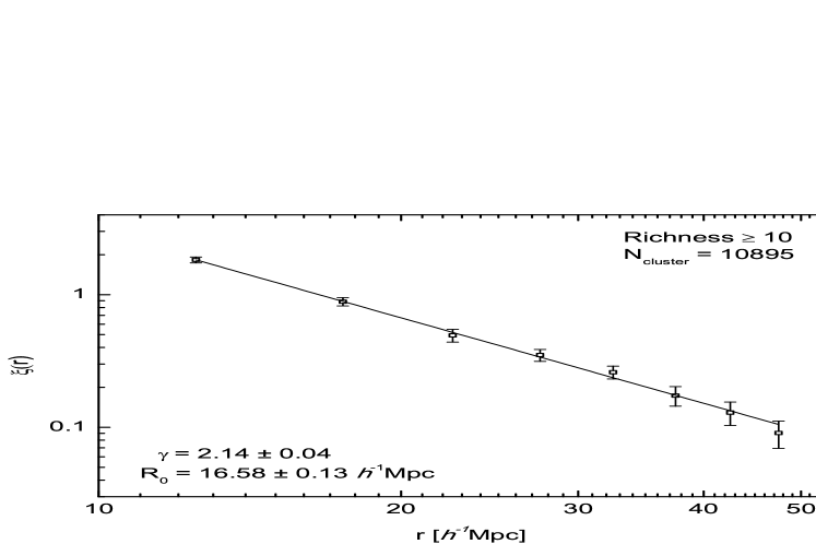
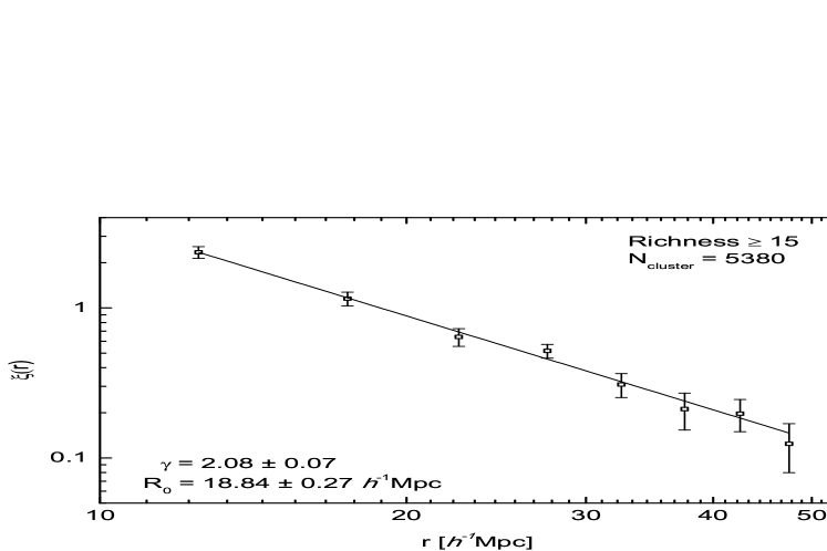
Figure 4.— Correlation function in the range $10~{}h^{-1}{\rm Mpc}\leq r\leq 50~{}h^{-1}{\rm Mpc}$ for clusters of three richness cutoffs. The solid line is the best fit of a power law.

We first analyze the correlation function on small scales. Bahcall & Soneira (1983) found that the correlation function of the Abell clusters is consistent with a power law on scales of less than several tens of $~{}h^{-1}{\rm Mpc}$. They also showed the correlation function is richness dependent, i.e. the correlation length increases with cluster richness. Their conclusions were confirmed by others using various cluster samples (Bahcall et al., 2003; Croft et al., 1997; Collins et al., 2000; Lee & Park, 2002; Estrada et al., 2009). The correlation function of the small scales ($r\leq 50~{}h^{-1}{\rm Mpc}$) can be fitted by the power law,

$$\xi(r)=\left(\frac{r}{R_{0}}\right)^{-\gamma},$$ (3)

where $R_{0}$ is the correlation length, $\gamma$ is the power law index. We calculate the correlation functions for our cluster sample with different thresholds of cluster richness (see Figure 4). Fitting the data with the power law in the range of $10~{}h^{-1}{\rm Mpc}\leq r\leq 50~{}h^{-1}{\rm Mpc}$, we get the values of $R_{0}$ and $\gamma$, as $R_{0}=18.84\pm 0.27~{}h^{-1}{\rm Mpc}$ and $\gamma=2.08\pm 0.07$ for 5 380 clusters with a richness of $R\geq 15$; $R_{0}=16.58\pm 0.13~{}h^{-1}{\rm Mpc}$ and $\gamma=2.14\pm 0.04$ for 10 895 clusters with $R\geq 10$; and $R_{0}=16.15\pm 0.13~{}h^{-1}{\rm Mpc}$ and $\gamma=2.11\pm 0.04$ for 13 884 clusters with $R\geq 5$. Our results are consistent with but more accurate than any previous works (i.e. Estrada et al., 2009, using maxBCG clusters). We find that the power index $\gamma$ almost does not change with the cluster richness, while the correlation length changes from $18.84~{}h^{-1}{\rm Mpc}$ for very rich clusters to $16.15~{}h^{-1}{\rm Mpc}$ for less rich clusters. We also find that the correlation length $R_{0}$ of clusters is considerably larger than those obtained from the galaxy samples, e.g. $5.91~{}h^{-1}{\rm Mpc}$ by Zehavi et al. (2004) using the volume limited SDSS galaxy sample, $R_{0}=5.05~{}h^{-1}{\rm Mpc}$ by Hawkins et al. (2003) using the 2dF galaxies.

4. Baryon acoustic oscillations and cosmological modeling

The correlation function shown in Figure  3 has an obvious excess around the $r\sim 110~{}h^{-1}{\rm Mpc}$ over the non-baryon model, which is the BAO feature in the large-scale structure of the universe. Here, we analyse the BAO feature using a $\Lambda$CDM model. To get the theoretical curve, we first obtain the linear matter power spectrum. The damped BAO feature has a non-linear evolution to each redshift in a $\Lambda$CDM model. We compute the redshift-space correlation functions at the central redshift of each counting bin between $z=0-0.4$ (see Figure 2), and then weight these functions using the corresponding number counts, i.e., the sample redshift distribution $n(z)$, to obtain the “averaged” correlation function. We finally fit this theoretical BAO model to real measurements, and constrain the cosmological parameters.

First, we compute the linear matter power spectra at each redshift using cmbfast (Zaldarriaga & Seljak, 2000). The damping of the BAO feature due to nonlinear evolution is approximated by an elliptical Gaussian (Eisenstein et al., 2007)

$$\tilde{P}(\mbox{{\emph{k}}})=\left(P_{\mathrm{lin}}(k)-P_{\mathrm{nw}}(k)\right)\exp{\left(-\frac{k_{\perp}^{2}\Sigma_{\perp}^{2}}{2}-\frac{k_{\parallel}^{2}\Sigma_{\parallel}^{2}}{2}\right)},$$ (4)

where $P_{\mathrm{lin}}(k)$ is the linear matter power spectrum, and $P_{\mathrm{nw}}(k)$ is the no-wiggle approximation of the linear matter power spectrum (Eisenstein & Hu, 1998). The rms of radial displacements across the line of sight is given by $\Sigma_{\perp}=\Sigma_{0}G$, where $\Sigma_{0}=11~{}h^{-1}{\rm Mpc}$, which is scaled from $12.4~{}h^{-1}{\rm Mpc}$ (Eisenstein et al., 2007) at $\sigma_{8}=0.9$ to $\sigma_{8}=0.8$ (Larson et al., 2011), and $G$ is the linear growth factor normalized as $G(z=0)=0.76$ in the reference cosmological model. The rms of radial displacements along the line of sight is $\Sigma_{\parallel}=\Sigma_{0}G(1+f)$), where $f=d(\ln G)/d(\ln a)\sim\Omega^{0.6}$ is the growth rate. Even though Equation (4) only involves the linear power spectra, the damping of the oscillating feature $\tilde{P}(\mbox{{\emph{k}}})$ is calculated based on $N$-body simulations. Hence, $\tilde{P}(\mbox{{\emph{k}}})$ needs not be subject to nonlinear mapping of the power spectrum again, though the difference is small in practice, whether it is mapped or not.

The nonlinear matter power spectrum is then given by the sum of the nonlinear no-wiggle matter power spectrum $P_{\mathrm{nl,nw}}(k)$ and the damped BAO feature $\tilde{P}(\mbox{{\emph{k}}})$

$$P_{\mathrm{nl}}(\mbox{{\emph{k}}})=\tilde{P}(\mbox{{\emph{k}}})+P_{\mathrm{nl,nw}}(k),$$ (5)

where we choose to use the Peacock & Dodds (1996) fitting formula to calculate $P_{\mathrm{nl,nw}}(k)$ for simplicity. Because the scales of interest are fairly large, different nonlinear fitting formulae produce very similar correlation functions at the end.

We next inlcude the linear redshift distortion effect (Kaiser, 1987) and nonlinear redshift distortion effect, along with the bias of galaxy cluster $b$, to obtain the power spetrum of galaxy clusters, $P_{\mathrm{c}}(k,\mu)$, in the redshift space

$$P_{\mathrm{c}}(k,\mu)=P_{\mathrm{nl}}(k,\mu)\frac{b^{2}(1+\beta\mu^{2})^{2}}{1+k^{2}\mu^{2}\sigma_{p}^{2}/2H^{2}},$$ (6)

where $\mu$ is the direction cosine. $\beta=f/b$ is the linear redshift distortion factor, $\sigma_{p}=400\mbox{km\,s}^{-1}$ denotes the pairwise velocity dispersion (see, e.g., Peacock et al., 2001). The denominator of Equation (6) models the finger-of-God effect or the nonlinear redshift distortion, which suppresses the power blow the cluster scale. Even though we measure correlations between clusters, the results may still be affected by the nonlinear redshift distortion because the redshift of each cluster is represented by the redshift of a single galaxy in most cases. In practice, however, we find that the nonlinear redshift distortion term in Equation (6) is unimportant for this work.

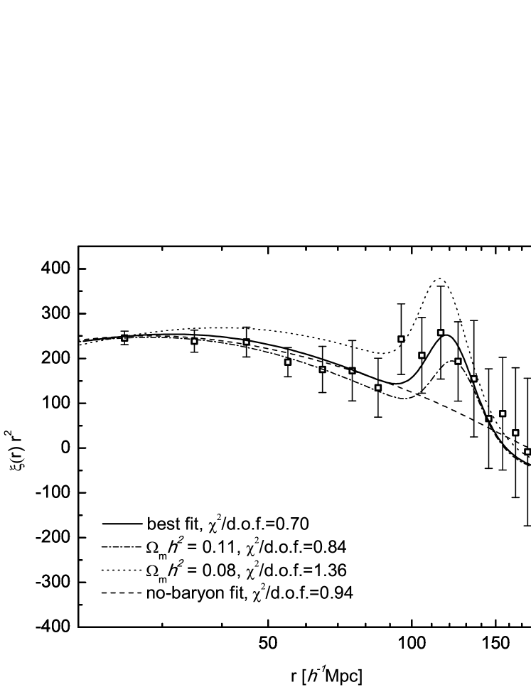
Figure 5.— The observed correlation function of 13 904 clusters in 18 bins from $20~{}h^{-1}{\rm Mpc}$ to $200~{}h^{-1}{\rm Mpc}$, together with the best-fit model curves with the BAO features (solid line) and without the BAO features (dashed line). The dot-dashed line ($\Omega_{m}h^{2}=0.11$) and dot line ($\Omega_{m}h^{2}=0.08$) outline two other models.

We multiply $b^{2}$ into the subsequent parentheses in Equation (6). By Fourier transforming this equation, we obtain the theoretical redshift-space two-point correlation function (monopole):

$$\xi=b^{2}\xi_{1}+b\xi_{2}+\xi_{3},$$ (7)

which consists of the components of the correlation function that have different dependence on the cluster bias. In this way, we can vary $b$ in the data fitting process efficiently.

Fitting the observed correlation function with theoretical curves is to compute $\chi^{2}$ using the full covariance matrix for a grid of parameters $\Omega_{m}h^{2},D_{v}(0.276)$ and $b$, where $D_{v}(z)$ is the reduced distance at the mean redshift of our sample $z_{m}=0.276$. $D_{v}(z)$ is firstly defined in Eisenstein et al. (2005) as,

$$D_{v}(z)=\left[D_{A}(z)^{2}{cz\over H(z)}\right]^{1/3},$$ (8)

where $H(z)$ is the Hubble parameter and $D_{A}(z)$ is the comoving angular diameter distance. For the reference cosmology, $\Omega_{m}=0.27$, $\Omega_{\Lambda}=0.73$, $h=0.71$ and $D_{v}^{ref}(0.276)=1072.5{~{}\rm Mpc}$. Note, the amplitude is not an independent parameter but its effect is included in the parameter $b$ here. The other involved cosmological parameters have been fixed to the WMAP7 (Larson et al., 2011) best-fit values: $\Omega_{b}=0.0449$, $n_{s}=0.96$ and $\sigma_{8}=0.8$.

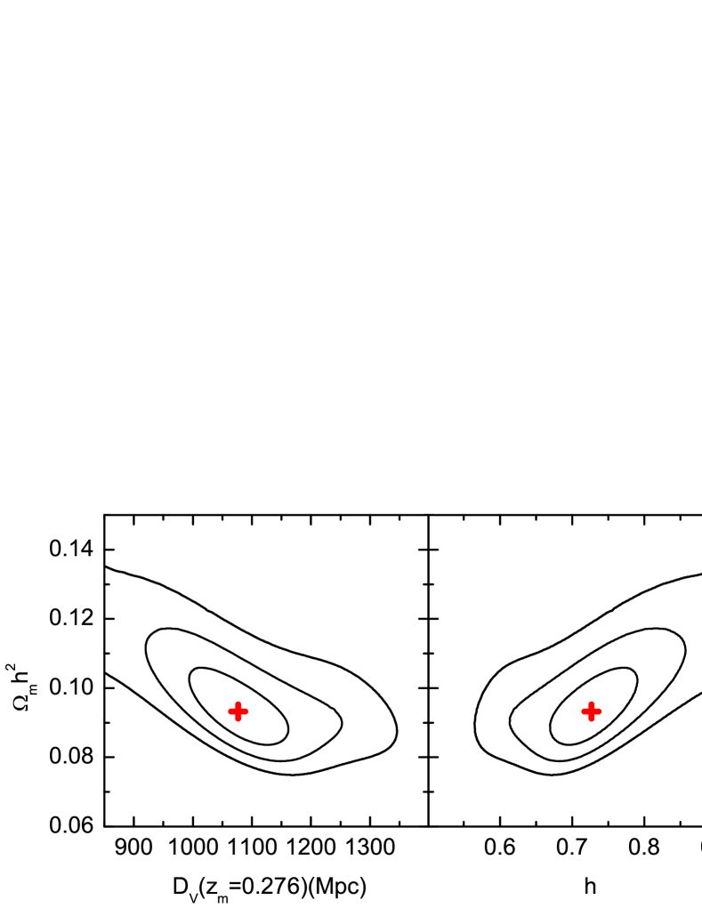
Figure 6.— Likelihood contours for the best-fit as $\Omega_{m}h^{2}=0.093$ and $D_{v}=1077{\rm Mpc}$ as a function of $D_{v}(z_{m}=0.276)$ and $\Omega_{m}h^{2}$ (left), and the likelihood contours for $h$ and $\Omega_{m}h^{2}$ (right). From the inner to the outer, contours corresponding to $1\sigma$, $2\sigma$, and $3\sigma$ respectively.

We do the $\chi^{2}$ search by scanning over a large table of $\Omega_{m}h^{2}$, $D_{v}(0.276)$ and b($0.05\leq\Omega_{m}h^{2}\leq 0.15$; $0.60\leq s=D_{v}^{ref}(0.276)/D_{v}(0.276)\leq 1.30$; $0.01\leq b\leq 3.75$). We then marginalize over $b$ by integrating the probability distribution $P(\Omega_{m}h^{2},D_{v},b)\propto Exp[-0.5\chi^{2}]$ along $b$-axis to give constraints on $\Omega_{m}h^{2}$ and $D_{v}$. The best-fit curve is shown in Figure 5, with the best-fit of $\chi^{2}=10.52$ on $15$ degrees of freedom (18 data points and 3 parameters; the reduced $\chi^{2}=0.70$). The best-fit pure CDM model without the BAO feature is also presented (the dashed line), which has a $\chi^{2}=14.02$ and is rejected at $1.87\sigma$. The marginalized constraints on $\Omega_{m}h^{2}$ and $D_{v}(0.276)$ are $D_{v}=1077\pm 55(1\sigma){~{}\rm Mpc}$ and $\Omega_{m}h^{2}=0.093\pm 0.0077(1\sigma)$ respectively, as shown in Figure 6. Assuming a flat cosmology with a cosmological constant model, there are only 2 degree of freedom of parameters in $D_{v}$ (indeed in $H(z)$). The constraints can be directly imposed on, say, $\Omega_{m}h^{2}-h$, so that we get $h=0.73\pm 0.039(1\sigma)$ (see Figure 6).

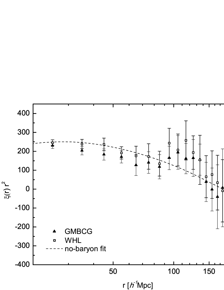
Figure 7.— The correlation function of clusters from the GMBCG sample (Hao et al., 2010) compared with that from Wen et al. (2009) cluster sample. The BAO features from the two samples are consistent.

Blake et al. (2011b) detected the BAO peak in the WiggleZ correlation functions for redshift slices of width $\Delta z=0.4$, which is the same width with our cluster sample. Blake et al. (2011b) fit these correlation functions using a four-parameter model, the fitting results are in agreement with WMAP 7-year value on $1\sigma$ level (see Table 2 in Blake et al., 2011b). Our cluster correlation function shows a more enhanced BAO peak than expected from the CMB model (see Figure 5). From the model-fitting to the correlation function of galaxy clusters, we get constraints of the distance-scale measurements $D_{v}(0.276)$ and $h$ which are consistent with WMAP 7-year results, while the constraint on $\Omega_{m}h^{2}$ is different from the widely accepted value obtained from the WMAP 7-year data ($\Omega_{m}h^{2}=0.133$, Larson et al., 2011). We have tested our analyzing algorithm by calculating and fitting the correlation functions of 160 LasDamas SDSS LRG mock catalogs (McBride et al. 2011, in preparation), and we found that our analysis method does not introduce any bias in the parameter estimation (see the Appendix for details).

In the very late stage of this work, Hao et al. (2010) published a new cluster catalog based on the BCG recognization and red-sequence features of galaxies, in which they identified 55 424 rich clusters in the redshift range $0.1<z<0.55$ from the SDSS DR7 data. Using their clusters, we get a sample of 15 074 clusters with available spectroscopical redshifts, which has almost the same sky coverage and redshift range as our sample. The correlation function of these 15 074 clusters as shown in Figure 7 is in good agreement with that from our cluster sample selected from Wen et al. (2009).

5. Summary

Galaxy clusters identified by Wen et al. (2009) from the SDSS cover a large scale area and have redshifts up to $z\sim 0.6$. We calculate the 2-point correlation function of a sample of clusters selected from Wen et al. (2009) to study the large-scale structure of the universe. To avoid the smearing effect from photometric redshift errors, clusters with at least one member galaxy spectroscopical observed for redshifts are selected. Our cluster sample contains 13 904 clusters of $z\leq 0.4$. The correlation function on the scales $10~{}h^{-1}{\rm Mpc}\leq r\leq 50~{}h^{-1}{\rm Mpc}$ of this cluster sample follows a power law. The power-law index about $\gamma=2.1$ is almost the same for the richer clusters and poorer clusters. The richer clusters have a larger correlation length. We get $R_{0}=18.84\pm 0.27~{}h^{-1}{\rm Mpc}$ for clusters of richness $R\geq 15$ and $R_{0}=16.15\pm 0.13~{}h^{-1}{\rm Mpc}$ for clusters of $R\geq 5$. This is consistent with but more accurate than previous results.

The correlation function on large-scale of $20~{}h^{-1}{\rm Mpc}\leq r\leq 200~{}h^{-1}{\rm Mpc}$ shows the baryon acoustic peak around $r\sim 110~{}h^{-1}{\rm Mpc}$ with a significance of $1.9\sigma$. We fit the observed correlation function with a parametrized theoretical curve, which is determined by the physical matter density parameter $\Omega_{m}h^{2}$, the stretch factor $s$, and the galaxy bias. We obtain the constraints $\Omega_{m}h^{2}=0.093\pm 0.0077(1\sigma)$, $D_{v}(0.276)=1077\pm 55(1\sigma){~{}\rm Mpc}$ and $h=0.73\pm 0.039(1\sigma)$.

Because the detected BAO peak in our cluster sample is stronger than expected, the estimated matter density parameter is more than $3\sigma$ lower than the WMAP 7-year result. It is unclear why the cluster correlation function shows the stronger BAO signal. Nevertheless, our results demonstrate that one can detect the BAO peak in the cluster correlation function at the expected scale. Future larger all sky spectroscopic galaxy and cluster surveys, such as BigBOSS (Schlegel et al., 2011), will provide deeper and more uniform spectroscopic samples of clusters for large-scale structure analysis, and can be used to verify the amplitude of BAO peak we detected.

Appendix A Testing the analyzing algorithm

We calculate and fit the correlation functions of 160 LasDamas mock catalogs to test our cosmological analyzing algorithm. The LasDamas simulation uses a single cosmological model with the same WMAP 5-year values of $\Omega_{m}=0.25$, $\Omega_{\Lambda}=0.75$, $\Omega_{b}=0.04$, $h_{0}=0.7$, $\sigma_{8}=0.8$ and $n_{s}=1.0$ (Komatsu et al., 2009). To build realistic SDSS mock catalogs, the LasDamas team places galaxies inside dark matter halos using a Halo Occupation Distribution with parameters from observed SDSS catalogs.

Figure 8.— The distribution of the ratio of the fitting parameter $\Omega_{m}$ and the fiducial $\Omega_{m}^{fid}$. The solid line is the best fit of a Gaussian function, the Gaussian fitting center is $[\Omega_{m}h^{2}/\Omega_{m}^{fid}h^{2}]_{center}=0.95$, with a $\sigma=0.15$. The mean value of 160 mock catalog fitting results is $[\Omega_{m}h^{2}/\Omega_{m}^{fid}h^{2}]_{mean}=0.99$.

Figure 9.— The distribution of the ratio of the fitting parameter $D_{v}$ and the fiducial $D_{v}^{fid}$. The solid line is the best fit of a Gaussian function, the Gaussian fitting center is $[D_{v}/D_{v}^{fid}]_{center}=0.97$, with a $\sigma=0.11$. The mean value of 160 mock catalog fitting results is $[D_{v}/D_{v}^{fid}]_{mean}=0.98$.

Figure 10.— The distribution of reduced $\chi^{2}$. The solid line is the best fit of a Gaussian function, the Gaussian fitting center is $\chi^{2}=1.13$, with a $\sigma=0.37$.

We build 160 testing mock catalogs by selecting 12 488 galaxies randomly from 160 different LasDamas LRG realizations which contain about 31 500 LRG galaxies ($M_{g}<-21.8$) respectively. All testing mock catalogs have the same footprint and redshift distribution with our cluster data catalog in the redshift region $0.16\leq z\leq 0.40$. The theoretical correlation function curve is calculated for the 160 testing mock catalogs with the same fiducial cosmological parameters of the LasDamas simulation using the method mentioned in Section 4.

Correlation functions are calculated for the 160 testing LRG mock catalogs respectively. By fitting these correlation functions with the theoretical curve, we find our analyzing algorithm works well. The statistical distribution of fitting parameters $\Omega_{m}$ and $D_{v}$ are shown in Figure 8 and Figure 9. We fit these distributions with a Gaussian function, the fitting centers are $\Omega_{m}/\Omega_{m}^{fid}=0.95\pm 0.15$ and $D_{v}/D_{v}^{fid}=0.97\pm 0.11$, which is consistent with the fiducial cosmology of the LasDamas mock catalogs. The distribution of 160 reduced $\chi^{2}$ is also shown in Figute 10.

References

- Abell (1958) Abell, G. O. 1958, ApJS, 3, 211
- Abell et al. (1989) Abell, G. O., Corwin, Jr., H. G., & Olowin, R. P. 1989, ApJS, 70, 1
- Bahcall et al. (2003) Bahcall, N. A., Dong, F., Hao, L., Bode, P., Annis, J., Gunn, J. E., & Schneider, D. P. 2003, ApJ, 599, 814
- Bahcall & Soneira (1983) Bahcall, N. A. & Soneira, R. M. 1983, ApJ, 270, 20
- Beutler et al. (2011) Beutler, F., et al. 2011, MNRAS, 416, 3017
- Blake & Bridle (2005) Blake, C. & Bridle, S. 2005, MNRAS, 363, 1329
- Blake et al. (2011a) Blake, C., et al. 2011a, MNRAS, 415, 2892
- Blake et al. (2011b) Blake, C., et al. 2011b, MNRAS, 418, 1707
- Colless et al. (2001) Colless, M., et al. 2001, MNRAS, 328, 1039
- Collins et al. (2000) Collins, C. A., et al. 2000, MNRAS, 319, 939
- Croft et al. (1997) Croft, R. A. C., Dalton, G. B., Efstathiou, G., Sutherland, W. J., & Maddox, S. J. 1997, MNRAS, 291, 305
- Csabai et al. (2003) Csabai, I., et al. 2003, AJ, 125, 580
- Eisenstein (2002) Eisenstein, D. 2002, in Astronomical Society of the Pacific Conference Series, Vol. 280, Next Generation Wide-Field Multi-Object Spectroscopy, ed. M. J. I. Brown & A. Dey, 35–+
- Eisenstein (2005) Eisenstein, D. J. 2005, New Astron. Rev., 49, 360
- Eisenstein & Hu (1998) Eisenstein, D. J. & Hu, W. 1998, ApJ, 496, 605
- Eisenstein et al. (2007) Eisenstein, D. J., Seo, H., & White, M. 2007, ApJ, 664, 660
- Eisenstein et al. (2005) Eisenstein, D. J., et al. 2005, ApJ, 633, 560
- Estrada et al. (2009) Estrada, J., Sefusatti, E., & Frieman, J. A. 2009, ApJ, 692, 265
- Gal et al. (2003) Gal, R. R., de Carvalho, R. R., Lopes, P. A. A., Djorgovski, S. G., Brunner, R. J., Mahabal, A., & Odewahn, S. C. 2003, AJ, 125, 2064
- Geller & Huchra (1989) Geller, M. J. & Huchra, J. P. 1989, Science, 246, 897
- Gott et al. (2005) Gott, III, J. R., Jurić, M., Schlegel, D., Hoyle, F., Vogeley, M., Tegmark, M., Bahcall, N., & Brinkmann, J. 2005, ApJ, 624, 463
- Hao et al. (2010) Hao, J., et al. 2010, ApJS, 191, 254
- Hawkins et al. (2003) Hawkins, E., et al. 2003, MNRAS, 346, 78
- Hütsi (2010) Hütsi, G. 2010, MNRAS, 401, 2477
- Kaiser (1987) Kaiser, N. 1987, MNRAS, 227, 1
- Kazin et al. (2010) Kazin, E. A., et al. 2010, ApJ, 710, 1444
- Koester et al. (2007a) Koester, B. P., et al. 2007a, ApJ, 660, 239
- Koester et al. (2007b) Koester, B. P., et al. 2007b, ApJ, 660, 221
- Komatsu et al. (2009) Komatsu, E., et al. 2009, ApJS, 180, 330
- Landy & Szalay (1993) Landy, S. D. & Szalay, A. S. 1993, ApJ, 412, 64
- Larson et al. (2011) Larson, D., et al. 2011, ApJS, 192, 16
- Lee & Park (2002) Lee, S. & Park, C. 2002, Journal of Korean Astronomical Society, 35, 111
- Lopes et al. (2004) Lopes, P. A. A., de Carvalho, R. R., Gal, R. R., Djorgovski, S. G., Odewahn, S. C., Mahabal, A. A., & Brunner, R. J. 2004, AJ, 128, 1017
- Martínez (2009) Martínez, V. J. 2009, in Lecture Notes in Physics, Berlin Springer Verlag, Vol. 665, Data Analysis in Cosmology, ed. V. J. Martínez, E. Saar, E. Martínez-González, & M.-J. Pons-Bordería, 269–289
- Miller et al. (2001) Miller, C. J., Nichol, R. C., & Batuski, D. J. 2001, ApJ, 555, 68
- Peacock et al. (2001) Peacock, J. A., et al. 2001, Nature, 410, 169
- Peacock & Dodds (1996) Peacock, J. A. & Dodds, S. J. 1996, MNRAS, 280, L19
- Peebles (1980) Peebles, P. J. E. 1980, The large-scale structure of the universe, ed. Peebles, P. J. E.
- Peebles & Yu (1970) Peebles, P. J. E. & Yu, J. T. 1970, ApJ, 162, 815
- Percival et al. (2010) Percival, W. J., et al. 2010, MNRAS, 401, 2148
- Schlegel et al. (2011) Schlegel, D., et al. 2011, ArXiv e-prints
- Sunyaev & Zeldovich (1970) Sunyaev, R. A. & Zeldovich, Y. B. 1970, Ap&SS, 7, 3
- Wen et al. (2009) Wen, Z. L., Han, J. L., & Liu, F. S. 2009, ApJS, 183, 197
- Wen et al. (2010) —. 2010, MNRAS, 407, 533
- York et al. (2000) York, D. G., et al. 2000, AJ, 120, 1579
- Zaldarriaga & Seljak (2000) Zaldarriaga, M. & Seljak, U. 2000, ApJS, 129, 431
- Zehavi et al. (2004) Zehavi, I., et al. 2004, ApJ, 608, 16
- Zhan et al. (2008) Zhan, H., Wang, L., Pinto, P., & Tyson, J. A. 2008, ApJ, 675, L1