Frasian Inference

Abstract

Don Fraser has given an interesting account of the agreements and disagreements between Bayesian posterior probabilities and confidence levels. In this comment I discuss some cases where the lack of such agreement is extreme. I then discuss a few cases where it is possible to have Bayes procedures with frequentist validity. Such frequentist-Bayesian—or Frasian—methods deserve more attention.

10.1214/11-STS352 Discussion of Is Bayes Posterior just Quick and Dirty Confidence? by D. A. S. Fraser

1 Introduction

Don Fraser has long advocated the idea that users of Bayesian methods have an obligation to study the frequentist properties of those methods. He makes the case quite forcefully when he states: “The failure to make true assertions with a promised reliability can be extreme with the Bayes use of mathematical priors” and, more ominously:

The claim of a probability status for a statement that can fail to approximate confidence is misrepresentation. In other areas of science such false claims would be treated seriously.

I completely agree with Don and I enjoyed reading his essay highlighting cases where approximate confidence does or does not hold. In this comment I will mention a few other places where Bayes methods have poor frequentist coverage. Then, on a more optimistic note, I’ll discuss a few cases where Bayes methods do have good frequentist properties. I’ll refer to these methods as Frasian, both to honor the author and as a handy way to refer to methods that meld frequentist guarantees with Bayesian ideas.

2 High-Dimensional Models

Don’s article shows that even in low-dimensional parametric models, Bayesian probability statements and confidence statements can diverge in nontrivial ways. The situation can be dramatically worse in high-dimensional and infinite dimensional models.

DKW versus DP

A simple example concerns estimating the cumulative distribution function $F$. Let $X_{1},\ldots,X_{n}\sim F$. Let $F_{n}(x)=\frac{1}{n}\sum_{i=1}^{n}I(X_{i}\leq x)$ be the usual empirical distribution function. By the famous DKW (Dvoretsky–Kiefer–Wolfowitz) inequality, we know that

$$\sup_{F}\mathbb{P}_{F}\Bigl{(}\sup_{x}|F_{n}(x)-F(x)|>\varepsilon\Bigr{)}\leq 2e^{-2n\varepsilon^{2}}.$$

Hence,

$$(L(x),U(x))$$

$$\quad\equiv\bigl{(}\max\{F_{n}(x)-\varepsilon_{n},0\},\min\{F_{n}(x)+\varepsilon_{n},1\}\bigr{)}$$

is a valid $1-\alpha$ confidence band, if we set $\varepsilon_{n}=\sqrt{\frac{1}{2n}\log(2/\alpha)}$. (Of course, narrower bands are possible.)

The usual Bayesian approach is the DP (Dirichlet Process) approach. Here, $F$ is a given Dirichlet process prior with mean $F_{0}$ and concentration parameter $\beta$, $F\sim\operatorname{DP}(F_{0},\beta)$. The posterior is $\operatorname{DP}(\overline{F}_{n},\beta+n)$ where $\overline{F}_{n}=\frac{\beta}{\beta+n}F_{0}+\frac{n}{\beta+n}F_{n}$. Let $(L,U)$ be a posterior $1-\alpha$ confidence band. In general, the coverage $\inf_{F}\mathbb{P}(L\leq F\leq U)$ is 0. This is a striking deviation from frequentist validity. The frequentist estimator can be recovered by formally letting $\beta\to 0$, although doing so is to just give up on Bayes.

Normal Means

Let $Y_{i}=\theta_{i}+\frac{1}{\sqrt{n}}\varepsilon_{i}$, $i=1,2,\ldots,$ where $\varepsilon_{1},\varepsilon_{2},\ldots$ are $N(0,1)$. This is the standard Normal means problem and many other problems, such as nonparametric regression, have been shown to be equivalent to this problem.

Suppose that $\theta=(\theta_{1},\theta_{2},\ldots)$ is in the Sobolev ellipsoid

$$\Theta=\Biggl{\{}\theta\dvtx\sum_{j=1}^{\infty}\theta_{i}^{2}i^{2p}\leq C^{2}\Biggr{\}}.$$

This corresponds to smooth regression functions in the nonparametric regression problem. The minimax rate is $n^{-2p/(2p+1)}$ and simple shrinkage estimators achieve this risk. Zhao (2000) and Shen and Wasserman (2001) showed that the priors that yield posterior that achieve the minimax rate are quite strange and unnatural and are never used in practice. The obvious prior—Normal on each coordinate—is not minimax unless we allow the prior to put zero mass on $\Theta$. This hints at the difficulties inherent in melding Bayes and frequentist ideas in high dimensions.

It gets worse when we look at the type of validity that Don focuses on. Can we find a prior in this problem such that the $1-\alpha$ posterior regions also have approximate $1-\alpha$ coverage? To the best of my knowledge, there is no definitive answer. But the results in Cox (1993) and Freedman (1999) suggest that the answer is no.

Missing Data and Causal Inference

Robins and Ritov (1997) construct an example that is motivated by missing data problems and causal inference problems. I refer the reader to their paper for details. But the punch line is dramatic. The frequentist interval (based on the Horwitz–Thompson estimator) shrinks at rate $O(1/\sqrt{n})$. For a Bayesian region to have correct coverage, its size will have to shrink no faster than a logarithmic rate. Hence, there is a drastic loss in efficiency if we want validity.

3 Frasian Inference

Is it possible to force Bayesian methods to have frequentist guarantees? Don’s article shows that the answer can be subtle. It depends on the structure of the model. Here I highlight two general techniques where we can force the Bayesian procedure to have finite sample frequentist guarantees.

Prediction

Let $\pi(\theta|Y^{n})\propto f(Y^{n}|\theta)\pi(\theta)$ denote the posterior where $Y^{n}=(Y_{1},\ldots,Y_{n})$. The predictive distribution for a new observation $Z$ (drawn from the same distribution as $Y^{n}$) is $\pi(z|Y^{n})=\int f(z|\theta)\pi(\theta|Y^{n})\,d\theta$. The usual Bayesian approach for prediction is to choose a set $B$ such that $\int_{B}\pi(y|Y^{n})\,dy=1-\alpha$. Of course, $B$ need not have frequentist coverage validity.

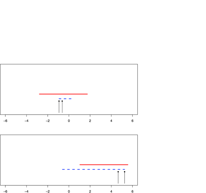
Figure 1: In the top plot $Y_{1},Y_{2}\sim N(0,1)$. In the bottom plot $Y_{1},Y_{2}\sim N(5,1)$. In both cases, the prior is $\theta\sim N(0,1)$. The two vertical lines show the locations of the two data points. The dashed horizontal line is the frequentized region. The solid horizontal line is Bayes predictive region.

But we can adapt the ideas in Vovk, Gammerman and Shafer (2005) to get a predictive region $A$ with finite sample frequentist validity. To construct $A$, we test the null hypothesis $H_{0}\dvtx Z=z$ using the Bayesian predictive density as a test statistic. We then invert the test to get $A$. Here are steps in detail:

1. [1.]

2. Fix $Z$ at some value $z$. [(a)]

3. Set $Y_{n+1}=z$ and form the augmented data set $Y_{1},\ldots,Y_{n},Y_{n+1}$.

4. Compute the predictive density $\pi(\cdot|Y_{1},\ldots,\allowbreak Y_{n},Y_{n+1})=\int f(\cdot|\theta)\pi(\theta|Y_{1},\ldots,Y_{n},Y_{n+1})\,d\theta$.

5. Compute the discrepancy statistics $D_{1},\ldots,\allowbreak D_{n+1}$ where $D_{i}\,{=}\,\pi(Y_{i}|Y_{1},\ldots,Y_{n},Y_{n+1}),i\,{=}\,1,\ldots,\allowbreak n+1$.

6. Compute the $p$-value $p(z)$ for testing $H_{0}\dvtx\allowbreak Z=z$ by

   $$p(z)=\frac{1}{n+1}\sum_{i=1}^{n}I(D_{i}\leq D_{n+1}).$$

   Under $H_{0}$, $D_{1},\ldots,D_{n+1}$ are exchangeable so this is a valid $p$-value.

7. After computing the $p$-value $p(z)$ for each value $z$, invert the test: let

   $$A=\{z\dvtx p(z)\geq\alpha\}.$$

It follows that

$$\mathbb{P}(Z\in A)\geq 1-\alpha.$$

This is true no matter what the prior is. In fact, it is true even if the model is wrong. Using the Bayesian predictive region as a test statistic is how we let the prior enter the problem. A good prior might lead to small prediction regions $A$. Thus, validity is guaranteed; only efficiency is in question. Here we are making use of the Bayesian machinery while maintaining frequentist validity. I will refer to $A$ as the frequentized region.

Figure 1 shows a toy example. The data are $N(\theta,1)$ and the prior is $\theta\sim N(0,1)$. To make the effect clear, we use a tiny sample size of $n=2$ and we use $\alpha=0.05$. The top plot shows the case where $\theta=0$ so the prior is consistent with the truth. The two vertical lines show the locations of the two data points. The dashed horizontal line is the frequentized region. The solid horizontal line is Bayes predictive region.

The second plot shows an example with $\theta=5$. Here there is a conflict between the prior and the truth. The Bayes region is shorter but of course does not have frequentist validity. The frequentized region is longer. This is the compensation for having a bad prior.

Weighted Hypothesis Testing

Consider testing $m$ null hypotheses $H_{01},\ldots,H_{0m}$ based on $p$-values $P_{1},\ldots,P_{m}$. The Bonferroni method takes the rejection set to be $R=\{j\dvtx P_{j}\leq\alpha/m\}$. It is well known that this procedure controls the error rate in the sense that

$$\mathbb{P}(R\cap\mathcal{H}_{0}\neq\varnothing)\leq\alpha,$$ (1)

where $\mathcal{H}_{0}=\{j\dvtx H_{0j}\mbox{ is true}\}$.

Suppose we have prior information that favors some of these null hypotheses. We could include this prior information by adopting a Bayesiananalysis. But then we lose the frequentist guarantee given in (1). Is there a way to tilt the analysis according to our prior information while preserving (1)? The answer is yes. Simply replace the $p$-values by weighted $p$-values $P_{j}/w_{j}$ and carry out the Bonferroni procedure. As long as the priorweights are non-negative and sum to one, then (1) still holds. (See Roeder and Wasserman, 2009, and Genovese, Roeder and Wasserman, 2006.) Although not formally a Bayesian procedure, it does allow us to have a nugget of Bayesianism by including prior weights while still preserving the frequentist guarantee.

For one-sided testing of Normal means, the optimal weights are $w_{j}=(m/\alpha)\overline{\Phi}(\theta_{j}/2+c/\theta_{j})$, where $\overline{\Phi}$ is the Gaussian survivor function and $c$ is the constant that makes the weights sum to one. The optimal weights depend on the unknown means $\theta_{j}$. Here is another opportunity to blend frequentist withBayes by using a prior on the $\theta_{j}$’s to optimize the weights.

4 Conclusion

Don Fraser has shown that, except in special circumstances, Bayesian posterior probabilities and frequentist confidence can diverge. The degree of divergence depends on features of the model such as nonlinearity.

I have discussed cases where the divergence can be extreme. On the other hand, I have also discussed some approaches for forcing Bayesian methods to have frequentist validity. But in general, we must be vigilant and pay careful attention to the sampling properties of procedures. Don’s paper is a useful reminder of the need for that vigilance.

References

- Cox (1993) {barticle}[mr] \bauthor\bsnmCox, \bfnmDennis D.\binitsD. D. (\byear1993). \btitleAn analysis of Bayesian inference for nonparametric regression. \bjournalAnn. Statist. \bvolume21 \bpages903–923. \biddoi=10.1214/aos/1176349157, issn=0090-5364, mr=1232525 \bptokimsref \endbibitem
- Freedman (1999) {barticle}[mr] \bauthor\bsnmFreedman, \bfnmDavid\binitsD. (\byear1999). \btitleOn the Bernstein–von Mises theorem with infinite-dimensional parameters. \bjournalAnn. Statist. \bvolume27 \bpages1119–1140. \bidissn=0090-5364, mr=1740119 \bptokimsref \endbibitem
- Genovese, Roeder and Wasserman (2006) {barticle}[mr] \bauthor\bsnmGenovese, \bfnmChristopher R.\binitsC. R., \bauthor\bsnmRoeder, \bfnmKathryn\binitsK. and \bauthor\bsnmWasserman, \bfnmLarry\binitsL. (\byear2006). \btitleFalse discovery control with -value weighting. \bjournalBiometrika \bvolume93 \bpages509–524. \biddoi=10.1093/biomet/93.3.509, issn=0006-3444, mr=2261439 \bptokimsref \endbibitem
- Robins and Ritov (1997) {barticle}[auto:STB—2011/08/02—11:14:52] \bauthor\bsnmRobins, \bfnmJ.\binitsJ. and \bauthor\bsnmRitov, \bfnmY.\binitsY. (\byear1997). \btitleToward a curse of dimensionality appropriate (coda) asymptotic theory for semi-parametric models. \bjournalStat. Med. \bvolume16 \bpages285–319. \biddoi=10.1002/(SICI)1097-0258(19970215)16:3 \bptokimsref \endbibitem
- Roeder and Wasserman (2009) {barticle}[mr] \bauthor\bsnmRoeder, \bfnmKathryn\binitsK. and \bauthor\bsnmWasserman, \bfnmLarry\binitsL. (\byear2009). \btitleGenome-wide significance levels and weighted hypothesis testing. \bjournalStatist. Sci. \bvolume24 \bpages398–413. \biddoi=10.1214/09-STS289, issn=0883-4237, mr=2779334 \bptokimsref \endbibitem
- Shen and Wasserman (2001) {barticle}[mr] \bauthor\bsnmShen, \bfnmXiaotong\binitsX. and \bauthor\bsnmWasserman, \bfnmLarry\binitsL. (\byear2001). \btitleRates of convergence of posterior distributions. \bjournalAnn. Statist. \bvolume29 \bpages687–714. \biddoi=10.1214/aos/1009210686, issn=0090-5364, mr=1865337 \bptokimsref \endbibitem
- Vovk, Gammerman and Shafer (2005) {bbook}[mr] \bauthor\bsnmVovk, \bfnmVladimir\binitsV., \bauthor\bsnmGammerman, \bfnmAlexander\binitsA. and \bauthor\bsnmShafer, \bfnmGlenn\binitsG. (\byear2005). \btitleAlgorithmic Learning in a Random World. \bpublisherSpringer, \baddressNew York. \bidmr=2161220 \bptokimsref \endbibitem
- Zhao (2000) {barticle}[mr] \bauthor\bsnmZhao, \bfnmLinda H.\binitsL. H. (\byear2000). \btitleBayesian aspects of some nonparametric problems. \bjournalAnn. Statist. \bvolume28 \bpages532–552. \biddoi=10.1214/aos/1016218229, issn=0090-5364, mr=1790008 \bptokimsref \endbibitem