Logarithmic relaxation and stress aging in the electron glass

Abstract

Slow relaxation and aging of the conductance are experimental features of a range of materials, which are collectively known as electron glasses. We report dynamic Monte Carlo simulations of the standard electron glass lattice model. In a non-equilibrium state, the electrons will often form a Fermi distribution with an effective electron temperature higher than the phonon bath temperature. We study the effective temperature as a function of time in three different situations: relaxation after a quench from an initial random state, during driving by an external electric field and during relaxation after such driving. We observe logarithmic relaxation of the effective temperature after a quench from a random initial state as well as after driving the system for some time $t_{w}$ with a strong electric field. For not too strong electric field and not too long $t_{w}$ we observe that data for the effective temperature at different waiting times collapse when plotted as functions of $t/t_{w}$ – the so-called simple aging. During the driving period we study how the effective temperature is established, separating the contributions from the sites involved in jumps from those that were not involved. It is found that the heating mainly affects the sites involved in jumps, but at strong driving, also the remaining sites are heated.

I Introduction

At low temperatures, disordered systems with localized electrons (e. g., located on dopants of compensated doped semiconductors or formed by Anderson localization in disordered conductors) conduct by phonon-assisted hopping. The theory of this process goes back to Mottmott who invented the concept of variable range hopping (VRH). In particular, he derived the Mott law for the temperature dependence of the conductance,

$$\sigma\propto\exp[-(\tilde{T}_{0}/T)^{1/(d+1)}],$$ (1)

where $T$ is temperature, $\tilde{T}_{0}$ is some characteristic temperature while $d$ is the dimensionality of the conduction problem. If Coulomb interactions are important one describes the system as an electron or Coulomb glass due to the slow dynamics at low temperatures.davies

As is well known (see Ref. ES, and references therein), the single-particle density of states (DOS) develops a soft gap at the Fermi level, the so called Coulomb gap.Pollak70 ; Pollak71 ; Srinivasan While this understanding of the density of states is generally accepted, the situation is less clear when it comes to describing dynamics in the interacting case. Using the Coulomb gap DOS in the VRH argumentsmott in the same way as the non-interacting DOS yields the Efros-Shklovskii (ES) law for conductance,ES75 ; ES76

$$\sigma\propto\exp[-(T_{0}/T)^{1/2}].$$ (2)

This has been observed experimentally in many different types of materials, like doped semiconductors,Zabrodskii93 ; Zhang93 ; Itoh96 ; Watanabe98 ; Massey00 granular metals adkins or two-dimensional systems.Shlimak ; Butko00

In recent years, there has been increasing interest in the non-equilibrium dynamics of hopping systems. In particular, the glass-like behavior at low temperatures has been studied both experimentally zvi ; ovadyahuPollak ; zviStressAging ; dragana ; grenet ; armitage ; borini and theoretically.markus ; ariel ; somoza In this work, we are interested in two features observed in the experiments. Firstly, it was observed that the conductivity relaxes logarithmically as a function of time after an initial quench or perturbation.ovadyahuPollak Secondly, if the system initially in equilibrium is perturbed by some change in external conditions (e. g., temperature or electric field) for a time $t_{w}$ called the waiting time, the relaxation back towards equilibrium of some quantity like the conductance $G(t,t_{w})$ will depend both on $t_{w}$ and the time $t$ since the end of the perturbation. It is found in certain cases that the relaxation is in fact described by a function $G(t/t_{w})$ of the ratio $t/t_{w}$. This behaviour is called simple aging.zviStressAging

While simple aging is observed in a range of different systems, we are here particularly concerned with experiments on disordered InO films.zvi One question which has been raised is whether the observed glassy behavior is an intrinsic feature of the electron system, or a result of some extrinsic mechanism like ionic rearrangement.zviIntrinsic In this work, we address the intrinsic mechanism by performing dynamical Monte Carlo simulations of the standard lattice model of the electron glass. It is known somoza that during a quench from an initial random state an effective electron temperature is quickly established, and that this temperature slowly relaxes to the bath temperature. We show that the electron temperature relaxes logarithmically over almost three decades in time and that the system demonstrates simple aging behavior in a stress aging protocol similar to what is seen in the experiments.zviStressAging While this does not constitute a proof of the intrinsic origin of the glassy behavior in the experiments on InO films, it shows that the model can display the observed behavior. To the best of our knowledge this was previously only demonstrated in a mean field approach,ariel the accuracy of which is not well understood.

II Model

We use the standard tight–binding Coulomb glass Hamiltonian,ES

$$H=\sum_{i}\epsilon_{i}n_{i}+\sum_{i<j}{\frac{(n_{i}-K)(n_{j}-K)}{r_{ij}}}\;,$$ (3)

$K$ being the compensation ratio. We take $e^{2}/d$ as our unit of energy where $d$ is the lattice constant which we take as our unit of distance. The number of electrons is chosen to be half the number of sites so that $K=1/2$. $\epsilon_{i}$ are random site energies chosen uniformly in the interval $[-U,U]$. In the simulations presented here we used $U=1$, which we know gives a well-developed Coulomb gap and the ES law for the conductance.tsigankov ; martin ; twoElectrons The sites are arranged in two dimensions on a $L\times L$ lattice where in all cases we used $L=1000$, which is sufficiently large to give a good estimate of the effective temperature in a single state without any averaging over a set of states. We implement cyclic boundary conditions in both directions.

To simulate the time evolution we used the dynamic Monte Carlo method introduced in Ref. tsigankov, . The basic idea of such simulations is to start the system in some particluar configuration. The configuration can change by one electron jumping from site $i$ to site $j$ (in principle, we should also take into account transitions involving two or more electrons jumping at the same time, but at the temperatures we consider here this should be a minor effect, see Ref. twoElectrons, and references therein for a discussion). The energy mismatch between the two states is supplied by the emission or absorption of a phonon, therefore the process is called phonon-assisted tunneling.

The rate of a phonon-assisted transition from site $i$ to site $j$ is usually specified as (see, e.g., Ref. ES, ),

$$\Gamma_{ij}\propto|\gamma_{q}|^{2}|N(\Delta E_{ij})|e^{-2r_{ij}/a}\,.$$ (4)

Here $\Delta E_{ij}$ is the phonon energy, $r_{ij}\equiv|\mathbf{r}_{i}-\mathbf{r}_{j}|$, $a$ is the localization length of the electronic state which we choose to 1, while $\gamma_{q}$ is a coupling constant, which in general depends on the wave vector $q$ of the involved phonon. Since $q\propto|\Delta E_{ij}|$ the pre-factor $\gamma_{q}$ leads to a power-law dependence of the transition rate on $|\Delta E_{ij}|$ where the power is model dependent. Since the power-law pre-exponential dependence does not change the results in a qualitative way we assume $\gamma_{q}$ to be $q$-independent. $N(E)=(e^{E/T}-1)^{-1}$ is the equilibrium phonon density. We set $k_{B}=1$ so that temperatures and energies are measured in the same units.

In the given initial state, one should, in principle, calculate all such rates, then select one at random weighted by the rates. The selected transition is then performed, all Coulomb energies recalculated, and the process repeated from the new state. Note that the rates depend on the states through the energy changes $\Delta E_{ij}$, which include the contributions from the Coulomb energy. All the rates therefore have to be recalculated at each step. In practice, one restricts the possible jumps by only considering those where the distance $r_{ij}$ is less than some maximal length (in our simulations we only considered jumps of less than 10 lattice units) since longer jumps become so improbable that they are never selected anyway. The procedure of selecting the next jump is also optimized in other ways, see Ref. tsigankov, and, in particular, Ref. tsigankovPRB, for a description of how to calculate the proper elapsed time. The only difference from Ref. tsigankov, is that following Ref. tenelsen, , we use for the transition rate $\Gamma_{ij}$ instead of (4) the approximate formula

$$\Gamma_{ij}={\tau_{0}}^{-1}e^{-2r_{ij}/a}\min\left(e^{-\Delta E_{ij}/T},1\right)$$ (5)

where $\Delta E_{ij}$ is the energy of the phonon and $r_{ij}$ is the distance between the sites. $\tau_{0}$ contains material dependent factors and energy dependent factors, which we approximate by their average value; we consider it as constant and its value, of the order of $10^{-12}$ s, is chosen as our unit of time. (Note that in Ref. tsigankov, a different approximate formula was used, we do not believe that the difference is of great significance, although it may change numerical values).

III Relaxation and effective temperature

To get more detailed understanding of how the effective temperature is established, we can follow the effective temperature as a function of time after an initial quench or some external perturbation like a strong electric field is applied.

Let us first relax from an initial random state and measure $T_{\text{eff}}(t)$. In all our simulations we used a phonon temperature $T=0.05$, which we know is well into the ES regime for VRH. The graphs show the evolution over $10^{8}$ jumps. Shown in Fig. 1 are the energy (inset) and the effective temperature as functions of time.

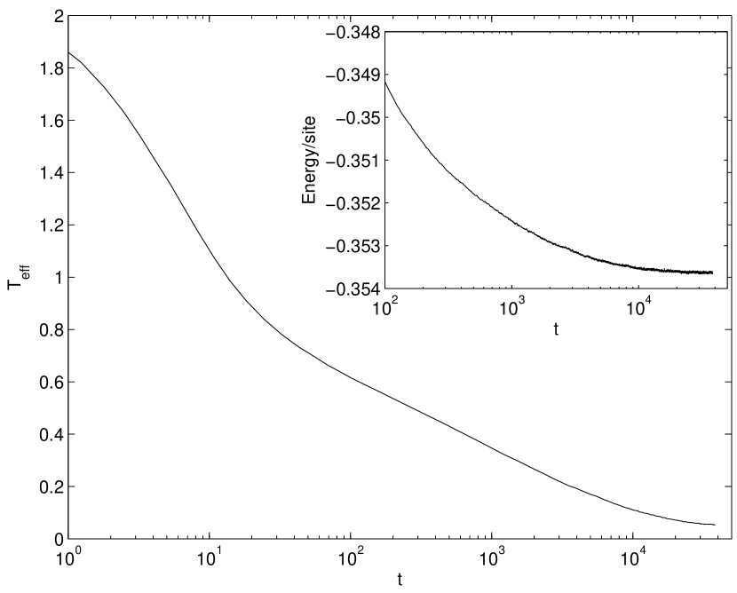
Figure 1: Effective temperature as function of time. The inset shows the energy as function of time.

As we can see, the energy graph has almost stopped to decrease, indicating that we have almost reached equilibrium. The same is seen by the effective temperature, where $T_{\text{eff}}=0.054$ in the final state. We see that the effective temperature, after some initial short time, logarithmically decreases in time for about two and a half orders of magnitude. The energy does not show this behavior (as discussed in Ref. martinRelax, , it is well fitted by a stretched exponential function). The relaxation of the effective temperature was studied previouslysomoza using a similar numerical method, but having the sites at random instead of on a lattice. A lower temperature was also used, and together this slows down the simulations so that only much smaller samples, up to 2000 sites, could be studied. Instead of out linear fit to effective temperature as a function of $\ln t$ they obtain a linear fit to effective temperature as a function of $1/\ln t$. The reason for this difference is not clear, but it may result from our larger samples and longer times.

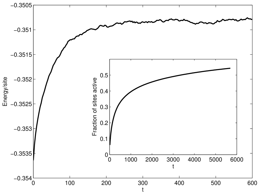
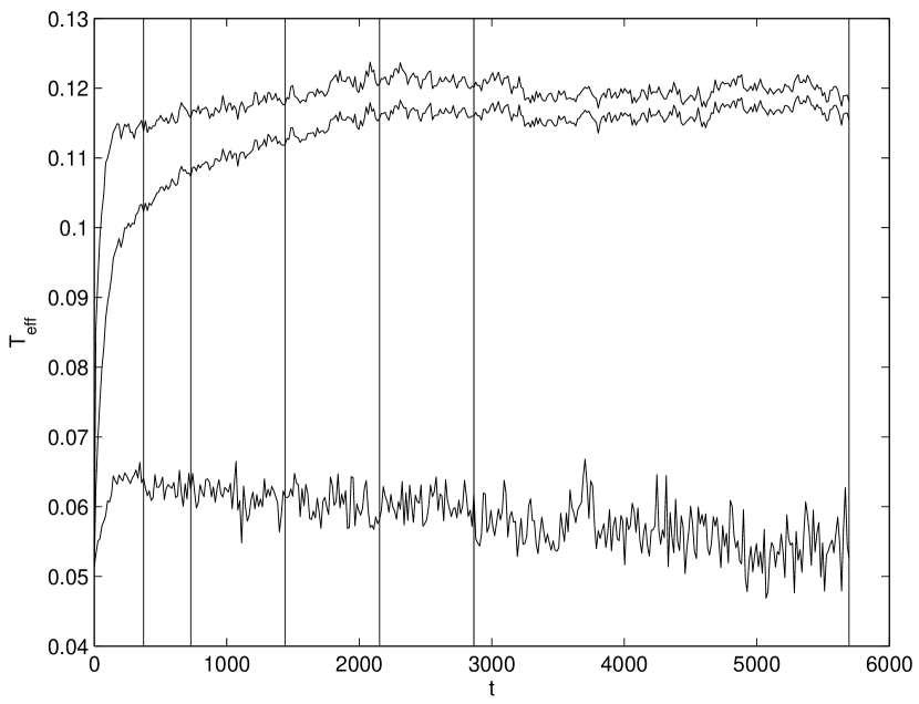
Figure 2: Top: Energy as function of time. Inset: The fraction of sites involved in a jump as function of time. Bottom: Effective temperature as function of time. The curves are from top to bottom the temperature of the sites which were active, the temperature of all sites and the temperature of the sites which were not active. The vertical lines indicate the waiting times in the stress aging protocol (see Fig. 5) .

Another type of experiment is to relax the system at low temperature and then apply a strong electric field to pump energy into the system. To equilibrate the system, we simulated the system with a localization length of 100, which facilitates long jumps and faster equilibration. When the energy did not decrease any more, we switched to the normal localization length of 1 and observed that the energy remained constant with fluctuations and $T_{\text{eff}}=0.05\pm 0.001$ after each $10^{6}$ jumps for a total of $7\cdot 10^{6}$ jumps. We then applied an electric field $E=0.1$ (in units of $e/d^{2}$). We know that Ohmic conduction takes place when $E\lesssim T/10$, so this should be well into the non-Ohmic regime and we expect the electron temperature to increase above the phonon temperature. Shown in the top panel of Fig. 2 is the energy per site as a function of time. The effective temperature as a function of time is shown in the lower panel (middle curve). Noting the difference in the timescales we conclude that the energy stabilizes at a new value much faster than the effective temperature.

We have also plotted the effective temperature taking into account only those sites which were involved in a jump, Fig. 2 (bottom, upper curve), and those which did not jump, Fig. 2 (bottom, lower curve). As we can see, the sites which are not involved in jumps are still at a temperature close to the phonon temperature. This is not a trivial statement, since the energies of the sites which are not involved in jumps also change due to the modified Coulomb interactions with the sites that jumped. Note that even at the latest time shown, new sites are still being involved, see Fig. 2 (top, inset), even if the energy and effective temperature are more or less stable.

The fitted Fermi functions are shown in Fig. 3.

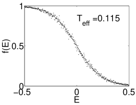
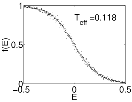
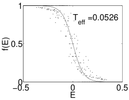
Figure 3: Fermi functions. Left: All sites, Center: Sites which took part in a transition, Right: Sites which did not take part in a transition. The points are the data and the curve the fitted function.

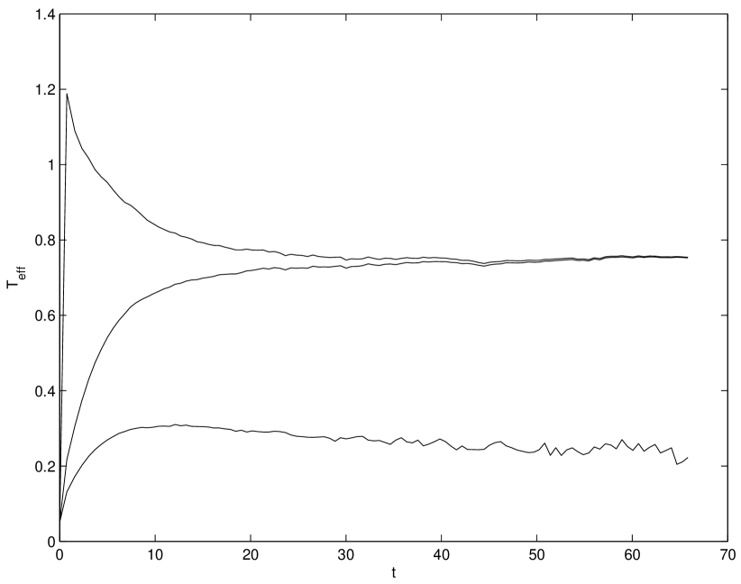
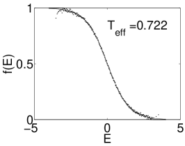
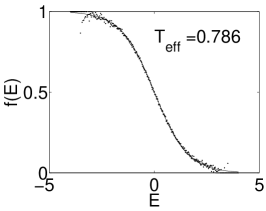
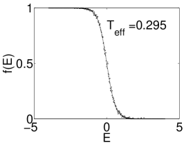
Figure 4: When driving with electric field $E=1$. Top: $T_{\text{eff}}$ as function of time. The curves are from top to bottom the temperature of the sites which were active, the temperature of all sites and the temperature of the sites which were not active. Bottom: Fitted Fermi functions at time $t=19$. Left: All sites, Center: Sites which took part in a transition, Right: Sites which did not take part in a transition. The points are the data and the curve the fitted function.

The fits are quite good, but the data for the sites which never were involved in jumps are more noisy. Note that the number of sites which jumped is still not much more than half the total number of sites, so the noise is not because there are few sites, but rather (as could be expected) that the sites which did not jump are those which are far from the Fermi level. These are either filled or empty and do not contribute much to the effective temperature. The noise indicates that the energy shifts are not correlated with the original energy of the site, so that there is no systematic change in the occupation probability giving a change in the effective temperature.

If we drive with a stronger field $E=1$ (Fig. 4), we observe two new features: First, the temperature of the sites which took part in a jump changes non-monotonously, first increasing rapidly and then decreasing towards a stationary value. Note however that at very short times, before the peak is reached, the distribution is not close to a Fermi distribution and the temperature is not a meaningful concept. On the decreasing part of the curve the Fermi function was already established. Second, we now observe significant heating also of the sites, which did not take part in a jump. Because of the Coulomb interaction it is not surprising that also these sites are affected by the transitions on other sites. What is surprising is that the occupation numbers still follow the Fermi distribution quite closely. Notice that the data are not noisy like in the case of weaker driving (Fig. 3), so the shifts in the energy levels are systematically adjusting to the Fermi distribution.

IV Stress Aging

Motivated by the logarithmic relaxation of effective temperature in Fig. 1 and using the heating curve of Fig 2 we will try to reproduce the experimental resultszviStressAging using the stress aging protocol. This means applying a non-Ohmic field for a certain time $t_{w}$ and then turning this field off (keeping only an Ohmic measuring field, which supposedly does not appreciably perturb the system). The heating process of Fig. 2 is exactly such a non-Ohmic driving, and we need only start simulations with zero fields at different points along this curve (in the experiments they kept an Ohmic measuring field, but since we are monitoring the effective temperature not the current this is not needed. We also ran simulations in Ohmic fields and confirmed that this did not appreciably affect the effective temperature as was expected). We have choosen six $t_{w}$, which correspond to the points marked on Fig. 2 with vertical lines.

Figure 5 (top) shows the effective temperature as function of time after the end of the driving period.

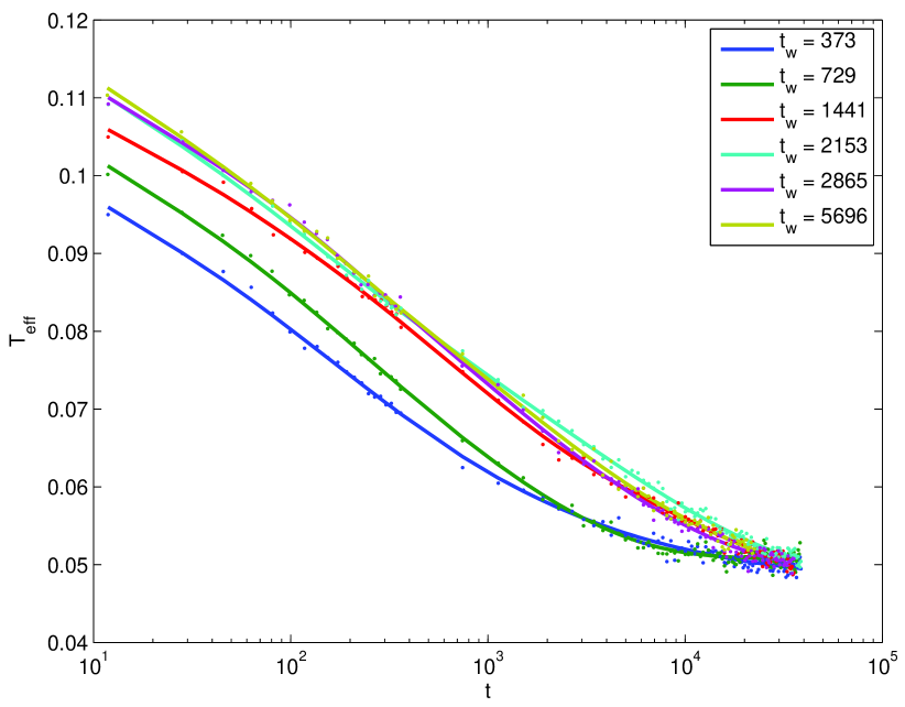
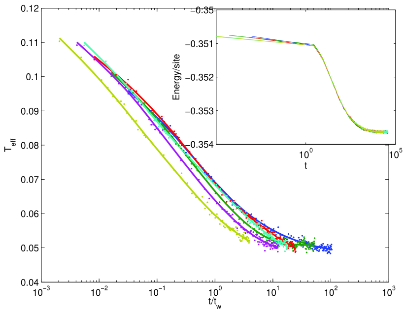
Figure 5: (Color online) After driving with $E=0.1$. Top: $T_{\text{eff}}$ as function of time. Bottom: $T_{\text{eff}}$ as function of $t/t_{w}$. Inset: Time dependences of the energy for different $t_{w}$.

Note that the time dependence of the energy is very similar in all cases as shown in Fig. 5 (bottom, inset). The effective temperature as a function of $t/t_{w}$ is shown in Fig. 5 (bottom).

From Fig. 5 we conclude that there is a logarithmic relaxation of the effective temperature after a driving by a non-Ohmic field just as in the case of relaxation from a random initial state (Fig. 1). Furthermore, we see that the curves for different $t_{w}$ collapse when time is scaled with $t_{w}$ when $t_{w}$ is smaller than some critical value $t_{w}^{(c)}\approx 2500$. The curve for $t_{w}=2865$ seems to lie a little to the left of the collapse curve, and for $t_{w}=5696$ this tendency is clear. The collpase of the curves for short $t_{w}$ is similar to what is observed in the experiments both on indium oxide filmszviStressAging and porous silicon.borini In the case of porous silicon, also the departure from the simple aging at longer waiting times was observed, while sufficiently long times were never reached in the case of indium oxide. If we compare to Fig. 2 (bottom) we see that the critical value $t_{w}^{(c)}$ corresponds to the time where the effective temperature stabilizes. Comparing to Fig. 2 (top) we see that this is a time much longer than the one, which is needed for the energy to stabilize.

To check that this behavior is not particular to one specific sample we repeated the procedure (relaxing to equilibrium using large localization length, then the stress aging protocol) on a different sample which gave similar results.

For the first sample we also repeated the stress aging protocol at different driving fields, $E=0.05$, 0.2, 0.5 and 1. Note that to be in the Ohmic regime we should have $E\lesssim T/10$, so all the fields are well outside of this. For $E=0.05$ the heating curve is shown in Fig. 6 (inset) and the effective temperature as function of time after the end of the driving period is shown in Fig. 6.

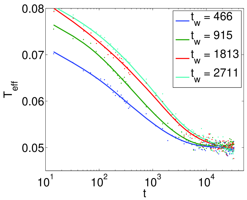
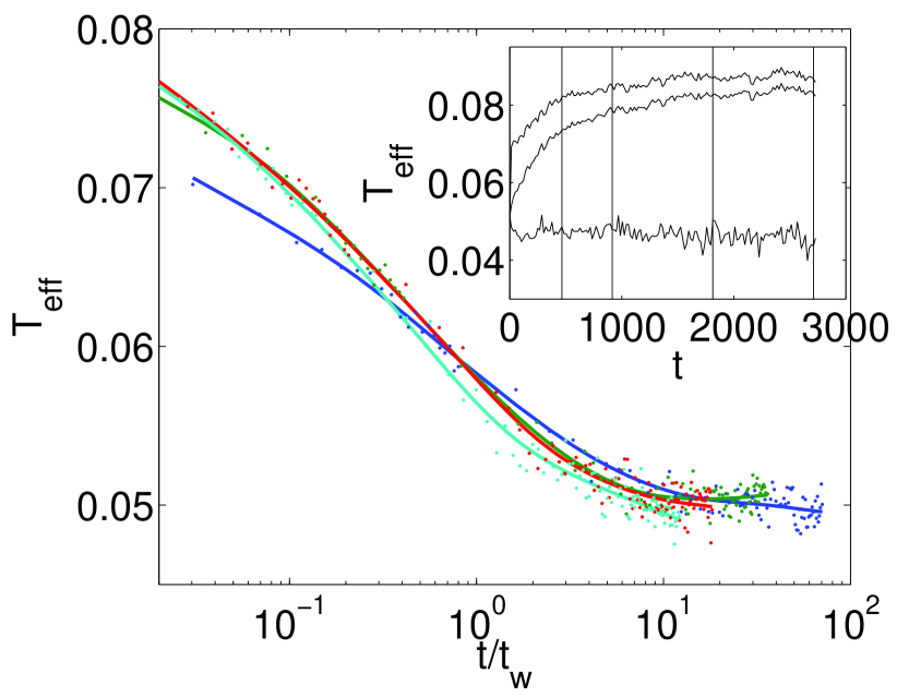
Figure 6: (Color online) After driving with $E=0.05$. Top: $T_{\text{eff}}$ as function of time. Bottom: $T_{\text{eff}}$ as function of $t/t_{w}$. Inset: The heating curve.

As we see, the general behavior is the same as when driving with $E=0.1$. For $E=0.2$ the heating curve is shown in Fig. 7 (inset) and the effective temperature as function of time after the end of the driving period is shown in Fig. 7.

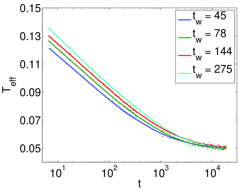
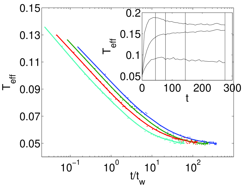
Figure 7: (Color online) After driving with $E=0.2$. Top: $T_{\text{eff}}$ as function of time. Bottom: $T_{\text{eff}}$ as function of $t/t_{w}$. Inset: The heating curve.

We see that the curves do not collapse satisfactorily, even for $t_{w}$ shorter than the time at which $T_{\text{eff}}$ stabilizes. This behavior is also observed in the experiments,zviStressAging it is characteristic for stronger fields.

Overall, what we observe is qualitatively very close to what is seen in experiments, but it should be noted that in experiments it is always the conductance that is measured, whereas we have studied the effective temperature. If we believe that the nonlinearity of the conductance is mainly due to heating of the electrons, then the nonlinear conductance can be found as the linear conductance, $\sigma_{0}$, at the effective temperature. It is known that this is approximately true.caravaca Based on this assumption and expecting that $\sigma_{0}(T_{\text{eff}})$ is an analytical function one would expect that $\Delta\sigma\equiv\sigma-\sigma_{0}(T)\propto T_{\text{eff}}-T$ at $T_{\text{eff}}-T\ll T$. This would be sufficient to show that the behavior of the conductivity would be the same as what we see for the effective temperature.

However, in our case $T_{\text{eff}}$ is significantly greater than $T$, and the above consideration seemingly does not work. Therefore we made an attempt to study conductivity directly. Instead of turning off the field after $t_{w}$ we switched to $E=0.005$ which should be more or less the highest field which is still in the Ohmic range. The effective temperature shows behavior which is similar to the one seen at $E=0$, which is what we expect since this field is so weak as to hardly affect the effective temperature.

To simulate the relaxation of conductivity is not so easy. Firstly, because to find the conductance, the system has to be followed over some time and transported charge measured. Usually it is noisy and one needs to average over a considerable time. With a large system like the one we have used, it is better, but still difficult to follow changes in the current. Secondly, and more importantly, when the strong, non-Ohmic field is applied, the system is polarized by charges shifting locally. These are charges which are not on the conducting path, and therefore they do not contribute to the DC current. But when the field is switched to a small, non-Ohmic value, these charges will flow backwards. Since we find the current by counting transferred charge in the direction of the field for each jump this will lead to a negative current for some time until this polarization has relaxed. One can ask whether this would also be seen in real experiments which only measures current in an external circuit. It seems that even if the localized charges are not on the conducting path, they would be capacitively coupled to the external circuit, and thereby detectable in real experiments. No such effect has been reported.

To see the relaxation of the conductivity, we took the accumulated transferred charge and subtracted the same in the absence of measuring field, which should contain only the relaxation of the polarization. The result was smoothed and the derivative calculated to find the current. The resulting curve showed some relaxation of the current, but the noise was too large and further work is needed in order to draw any clear conclusions.

V Discussion

The phenomenology observed in our simulations agrees with what is seen in the experiments zviStressAging ; borini in virtually all essential aspects: We observe logarithmic relaxation of the effective temperature after a quench from a random initial state. We also observe logarithmic relaxation after driving the system for some time $t_{w}$ with a strong electric field. When the driving field is not too strong and $t_{w}$ not too long we observe simple aging in the sense that the curves for different waiting times collapse on a common curve when plotted as functions of $t/t_{w}$. When $t_{w}$ exceeds some critical value, $t_{w}^{(c)}$, the scaled curves do not follow the common curve. When the driving field is large the curves do not collapse even for short times. The only difference is that while in the experiments conductance was measured, we have studied the effective temperature. We have to rely on the assumption that the conductance is given by the linear conductance at the effective temperature to relate our results to the experiments.

The aging protocol discussed here is the subject of a recent mean field analysis.ariel ; borini It predicts the relaxation of the average occupation number after the field is turned off. It is then argued that the excess current should follow the same law,

$$\delta\sigma\sim\int_{\lambda_{\min}}^{\lambda_{\max}}\frac{d\lambda}{\lambda}\left(1-e^{-\lambda t_{w}}\right)e^{-\lambda t_{w}}\,,$$

where $\lambda_{\min}$ and $\lambda_{\max}$ are the slowest and fastest modes. If we assume that $\lambda_{\max}t\gg 1$ we can set $\lambda_{\max}=\infty$ and we get

$$\delta\sigma\sim E_{1}(\lambda_{\min}t)-E_{1}[\lambda_{\min}(t+t_{w})]$$ (6)

where $E_{1}(x)=\int_{x}^{\infty}t^{-1}e^{-t}\,dt$ is the exponential integral function. Its series expansion is $E_{1}(x)=-\ln x-\gamma+x+\ldots$ so that for $t,t_{w}\ll/\lambda_{\min}$ we get $\delta\sigma\sim\ln(1+t_{w}/t)$. When $t\ll t_{w}$ it reduces to what we have used before. The idea is that the failure to collapse the curves for long $t_{w}$ is because $\lambda_{\min}t_{w}\gtrsim 1$ and we have to use the full exponential integral instead of only the leading logarithmic term. Assuming the excess effective temperature follows the same law as the conductance we should plot $\delta T=T_{\text{eff}}-T$ as function of $E_{1}(\lambda_{\min}t)-E_{1}[\lambda_{\min}(t+t_{w})]$ and obtain a collapse of the curves to a straight line (Fig. 8). This was indeed observed in the experiments on porous silicon.borini $\lambda_{\min}$ is now a fitting parameter, which we fit by hand to find the best collapse when $\lambda_{\min}=2.5\cdot 10^{-4}$. This agrees at least approximately with the idea that $1/\lambda_{\min}=4000$ should be not far from the $t_{w}^{(c)}=2500$ that we found above. The collapse is not to a straight line, but rather close to a square root. We can see this clearer if we plot (Fig. 8, inset) $\delta T^{2}$ as function of $E_{1}(\lambda_{\min}t)-E_{1}[\lambda_{\min}(t+t_{w})]$.

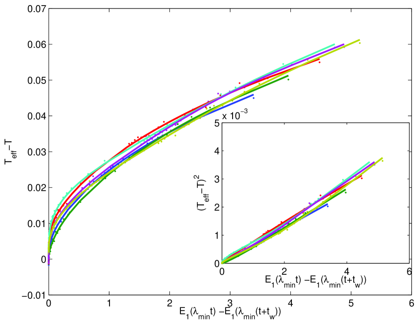
Figure 8: (Color online) $\delta T$ as function of $E_{1}(\lambda_{\min}t)-E_{1}[\lambda_{\min}(t+t_{w})]$. Inset: $\delta T^{2}$ as function of $E_{1}(\lambda_{\min}t)-E_{1}[\lambda_{\min}(t+t_{w})]$ after driving with $E=0.1$. The data are the same as in Fig. 5 and the color labels are the same.

All the curves fall close to the straight line indicating that the scaling relation predicted by the mean field theory is respected by our data. However, we can ask why $\delta T^{2}$ rather than $\delta T$ fall on a straight line. If we believe that our numerical model is applicable to the experiments, it seems to indicate that $\delta\sigma\propto\delta T^{2}$ instead of $\delta\sigma\propto\delta T$ as we obtained above from the assumption that the conductance is the linear conductance at the effective temperature and $\delta T/T\ll 1$.

VI Conclusions

We have demonstrated logarithmic relaxation of the effective temperature after a quench from a random initial state. The same is observed after driving by some non-Ohmic electric field. In the latter case we also observe simple aging when the driving field is not too strong and the waiting time not too long. At longer waiting times or after driving with stronger electric fields we observe departure from the simple aging qualitatively similar to what is seen in experiments.

The Monte Carlo approach allows us to access several properties, which are not available either in the experiments or the mean field theory. When applying a non-Ohmic field both the average energy and the effective temperature increase and saturate at a level above the equilibrium one. We find that the saturation of energy is much faster than the saturation of effective temperature.

We also see that the heating mainly affects those sites which were involved in jumps. At moderate driving fields the energies of the remaining sites are shifted by the changing Coulomb interactions, but there is no sytematic shifts, and the best fitting Fermi distribution is still at or close to the bath temperature. At stronger fields there is also some heating of the sites which were not involved in jumps, and the distribution still follows a Fermi function.

References

- (1) N. F. Mott, J. Non-Cryst. Solids 1, 1 (1968).
- (2) J. H. Davies, P. A. Lee, and T. M. Rice, Phys. Rev. Lett. 49, 758 (1982).
- (3) B. I. Shklovskii and A. L. Efros, Electronic properties of doped semiconductors (Springer, Berlin, 1984).
- (4) M. Pollak, Discuss. Faraday Soc. 50, 13 (1970).
- (5) M. Pollak, Proc. R. Soc. London, Ser. A 325, 383 (1971).
- (6) G. Srinivasan, Phys. Rev. B 4, 2581 (1971).
- (7) A. L. Efros and B. I. Shklovskii, J. Phys. C 8, L49 (1975).
- (8) A. L. Efros, J. Phys. C 9, 2021 (1976).
- (9) A. G. Zabrodskii and A. G. Andreev, JETP Lett., 58, 756 (1993).
- (10) J. Zhang, et al., Phys. Rev. B, 48, 2312 (1993).
- (11) K. M. Itoh, et al., Phys. Rev. Lett., 77, 4058 (1996).
- (12) M. Watanabe, et al., Phys. Rev. B, 58, 9851 (1998).
- (13) J. G. Massey and M. Lee, Phys. Rev. B, 62, R13270 (2000).
- (14) C. J. Adkins, J. Phys.: Cond. Matt. 1, 1253 (1989).
- (15) I. Shlimak, et al., Phys. Rev. B, 61, 7253 (2000).
- (16) V. Y. Butko, J. F. DiTusa and P. W. Adams, Phys. Rev. Lett. 84, 1543 (2000).
- (17) A. Vaknin, Z. Ovadyahu, and M. Pollak, Phys. Rev. Lett. 84, 3402 (2000); Phys. Rev. B, 65, 134208 (2002).
- (18) Z. Ovadyahu and M. Pollak, Phys. Rev. B 68, 184204 (2003).
- (19) V. Orlyanchik and Z. Ovadyahu, Phys. Rev. Lett. 92, 066801 (2004).
- (20) S. Bogdanovich and D. Popović, Phys. Rev. Lett. 88, 236401 (2002); J. Jaroszyński and D. Popović, Phys. Rev. Lett. 96, 037403 (2006).
- (21) T. Grenet , J. Delahaye, M. Sabra, and F. Gay, Eur. Phys. J. B 56, 183 (2007).
- (22) V. K. Thorsmølle and N. P. Armitage, Phys. Rev. Lett. 105, 086601 (2010).
- (23) Ariel Amir, Stefano Borini, Yuval Oreg, and Yoseph Imry, Phys. Rev. Lett. 107, 186407 (2011).
- (24) M. Müller and L. B. Ioffe, Phys. Rev. Lett. 93, 256403 (2004). Eran Lebanon and Markus Müller, Phys. Rev. B 72, 174202 (2005).
- (25) Ariel Amir, Yuval Oreg, and Yoseph Imry, Phys. Rev. Lett. 103, 126403 (2009).
- (26) A. M. Somoza, M. Ortuño, M. Caravaca, and M. Pollak Phys. Rev. Lett. 101, 056601 (2008).
- (27) Z. Ovadyahu, Phys. Rev. B 78, 195120 (2008).
- (28) D. N. Tsigankov and A. L. Efros, Phys. Rev. Lett. 88, 176602 (2002).
- (29) A. Glatz, V. M. Vinokur, J. Bergli, M. Kirkengen, and Y. M. Galperin J. Stat. Mech. P06006 (2008).
- (30) J. Bergli, A. M. Somoza, and M. Ortuño Phys. Rev. B 84, 174201 (2011).
- (31) D. N. Tsigankov, E. Pazy, B. D. Laikhtman, and A. L. Efros, Phys. Rev. B, 68 184205 (2003).
- (32) K. Tenelsen and M. Schreiber, Phys. Rev. B 52, 13287 (1995); A. Díaz-Sánchez et. al., Phys. Rev. B 59, 910 (1999).
- (33) M. Kirkengen and J. Bergli Phys. Rev. B 79, 075205 (2009).
- (34) M. Caravaca, A. M. Somoza, and M. Ortuño, Phys. Rev. B 82, 134204 (2010).