Mesoscopic Anderson Box: Connecting Weak to Strong Coupling

Abstract

We study the Anderson impurity problem in a mesoscopic setting, namely, the “Anderson box” in which the impurity is coupled to finite reservoir having a discrete spectrum and large sample-to-sample mesoscopic fluctuations. Note that both the weakly coupled and strong coupling Anderson impurity problems are characterized by a Fermi-liquid theory with weakly interacting quasiparticles. We study how the statistical fluctuations in these two problems are connected, using random matrix theory and the slave boson mean field approximation (SBMFA). First, for a resonant level model such as results from the SBMFA, we find the joint distribution of energy levels with and without the resonant level present. Second, if only energy levels within the Kondo resonance are considered, the distributions of perturbed levels collapse to universal forms for both orthogonal and unitary ensembles for all values of the coupling. These universal curves are described well by a simple Wigner-surmise-type toy model. Third, we study the fluctuations of the mean field parameters in the SBMFA, finding that they are small. Finally, the change in the intensity of an eigenfunction at an arbitrary point is studied, such as is relevant in conductance measurements. We find that the introduction of the strongly-coupled impurity considerably changes the wave function but that a substantial correlation remains.

I Introduction

The Kondo problem Kondo (1964); Hewson (1993), namely the physics of a magnetic impurity weakly coupled to a sea of otherwise non-interacting electrons, is one of the most thoroughly studied questions of many-body solid state physics. One reason for this ongoing interest is that the Kondo problem is a deceptively simple model system which nevertheless displays very non-trivial behavior and so requires the use of a large variety of theoretical tools to be thoroughly understood, including exact approaches (the numerical renormalization group Wilson (1975); Bulla et al. (2008), Bethe ansatz techniques Andrei (1980); Wiegmann (1980), and bosonization Giamarchi (2004); Schotte and Schotte (1969); Schotte (1970); Blume et al. (1970)) as well as various approximation schemes (perturbative renormalization Anderson (1970); Fowler and Zawadowzki (1971) and mean field theories Lee et al. (2006); Lacroix and Cyrot (1979); Coleman (1983); Read et al. (1984)).

In its original form, the Kondo problem refers to a dilute set of real magnetic impurities (e.g. Fe) in some macroscopic metallic host (say Au). In such circumstances, the density of states of the metallic host can be considered as flat and featureless within the energy scale at which the Kondo physics takes place. Modeling that case with a simple impurity model such as either the $s$-$d$ model or the Anderson impurity model Hewson (1993), one finds that a single energy scale, the Kondo temperature $T_{\rm K}$, emerges and distinguishes two rather different temperature regimes. For temperatures $T$ much larger than $T_{\rm K}$, the magnetic impurity behaves as a free moment with an effective coupling which, although renormalized to a larger value than the (bare) microscopic one, remains small. For $T\ll T_{\rm K}$ on the other hand, the magnetic impurity is screened by the electron gas and the system behaves as a Fermi liquid Nozières (1974) characterized by a phase shift and a residual interaction associated with virtual breaking of the Kondo singlet.

That the Kondo effect is in some circumstances relevant to the physics of quantum dots was first theoretically predicted Ng and Lee (1988); Glazman and Raikh (1988) and then considerably later confirmed experimentally Goldhaber-Gordon et al. (1998); Cronenwett et al. (1998); van der Wiel et al. (2000). Indeed, for temperatures much lower than both the mean level spacing and the charging energy, a small quantum dot in the Coulomb blockade regime can be described by the Anderson impurity model, with the dots playing the role of the magnetic impurity and the leads the role of the electron sea. Quantum dots, however, bring the possibility of two novel twists to the traditional Kondo problem. The first follows from the unprecedented control over the shape, parameters, and spatial organization of quantum dots: such control makes it possible to design and study more complex “quantum impurities” such as the two-channel, two impurity, or SU(4) Kondo problems Grobis et al. (2007); Chang and Chen (2009). The second twist, which shall be our main concern here, is that the density of states in the electron sea may have low energy structure and features, in contrast to the flat band typical of the original Kondo effect in metals.

Indeed, the small dot playing the role of the quantum impurity need not be connected to macroscopic leads, but rather may interact instead with a larger dot. The larger dot may itself be large enough to be modeled by a sea of non-interacting electrons (perhaps with a constant charging energy term) but, on the other hand, be small enough to be fully coherent and display finite size effects Kouwenhoven et al. (1997). These finite size effects introduce two additional energy scales into the Kondo problem. The first is simply the existence of a finite mean level spacing, leading to what has been called the “Kondo box” problem by Thimm and coworkers Thimm et al. (1999). The other energy scale introduced by the finite electron sea is the Thouless energy $E_{\rm Th}=\hbar/\tau_{c}$ where $\tau_{c}$ is the typical time to travel across the “electron-reservoir” dot. When probed with an energy resolution smaller than $E_{\rm Th}$, both the spectrum and the wave-functions of the electron sea display mesoscopic fluctuations Kouwenhoven et al. (1997), which will affect the Kondo physics and hence lead to what has been called the “mesoscopic Kondo problem” Kaul et al. (2005). Similar studies were also conducted in the context of disordered systems Kettemann (2004); Kettemann and Mucciolo (2006).

Both the Kondo box problem and the high temperature regime of the mesoscopic Kondo problem are by now reasonably well understood. For a finite but constant level spacing in the large dot, various theoretical approaches ranging from the non-crossing approximation Thimm et al. (1999) and slave boson mean field theory Simon and Affleck (2003) to exact quantum Monte Carlo Yoo et al. (2005); Kaul et al. (2006, 2009) and numerical renormalization group methods Cornaglia and Balseiro (2002a, b, 2003) have been used to map out the effect on the spectral function Cornaglia and Balseiro (2002b), persistent current Kang and Shin (2000); Affleck and Simon (2001), conductance Simon and Affleck (2002); Simon et al. (2006); Pereira et al. (2008), and magnetization Cornaglia and Balseiro (2002a); Kaul et al. (2006, 2009). In the same way, a mix of perturbative renormalization group analysis Zaránd and Udvardi (1996); Kaul et al. (2005); Bedrich et al. (2010) and quantum Monte Carlo Kaul et al. (2005) have made it possible to understand the high temperature regime of the mesoscopic problem (see also Refs. Kettemann, 2004; Kettemann and Mucciolo, 2006, 2007; Zhuravlev et al., 2007 for treatment of disordered systems). The picture that emerges is that mesoscopic fluctuations of the density of states translate into mesoscopic fluctuations of the Kondo temperature, but that once this translation has been properly taken into account, the high-temperature physics remains essentially the same as in the flat band case. In particular, physical properties can be written as the same universal function of the ratio $T/T_{\rm K}$ as in the bulk flat-band case, as long as $T_{\rm K}$ is understood as a realization dependent parameter Kaul et al. (2005). In this sense, the Kondo temperature remains a perfectly well defined concept (and quantity) in the mesoscopic regime, as long as it is defined from the high-temperature behavior.

In contrast, the consequences of mesoscopic fluctuations on Kondo physics in the low temperature regime, $T\!\ll\!T_{\rm K}$, remain largely unexplored. A few things are nevertheless known: for instance, using the example of the local susceptibility, exact Monte Carlo calculations have confirmed that below $T_{\rm K}$ physical quantities do not have the universal character typical of the traditional (flat band) Kondo problem Kaul et al. (2005). This result is not surprising since the mesoscopic fluctuations existing at all scales between the mean level spacing $\Delta$ and $E_{\rm Th}$ introduce in some sense a much larger set of parameters in the definition of the problem, leaving no particular reason why all physical quantities should be expressed in terms of $T/T_{\rm K}$. Thus, the low temperature regime of the mesoscopic Kondo problem should display non-trivial but interesting features. On the other hand, it seems reasonably clear that the very low temperature regime should be described by a Nozières-Landau Fermi liquid, as in the original Kondo problem. Indeed, the physical reasoning behind the emergence of Fermi liquid behavior at low temperatures, namely that for energies much lower than $T_{\rm K}$ the impurity spin has to be completely screened, applies as well in the mesoscopic case as long as $T,\Delta\ll T_{\rm K}$.

As a consequence, the mesoscopic Kondo problem provides an interesting example of a system which, as the temperature is lowered, starts as a (nearly) non-interacting electron gas with some mesoscopic fluctuations when $T\gg T_{\rm K}$, goes through an intrinsically correlated regime for $T\simeq T_{\rm K}$, and then becomes again a non-interacting electron gas (essentially) with a priori different mesoscopic fluctuations as $T$ becomes much smaller than $T_{\rm K}$. A natural question, then, is to characterize the correlation between the statistical fluctuations of the electron gas corresponding to the two limiting regimes. The goal of this paper is to address this issue (some preliminary results were reported in Ref. Liu et al., 2012). As an exact treatment of the low temperature mesoscopic Kondo problem is not an easy task, we shall tackle this problem here in a simplified framework, namely the one of slave boson/fermion mean field theory, within which a complete understanding can be obtained. We shall furthermore limit our study to the case where the dynamics in the finite “electron sea” reservoir is chaotic, and thus the statistical fluctuations of the high temperature Fermi gas is described by random matrix theory Bohigas (1991).

The structure of this paper is as follows. In Sec. II, we introduce more formally the mesoscopic Kondo model under study and describe the mean field approach on which the analysis is based. Sec. III is devoted to the fluctuations of the mean field parameters. Fluctuations of physical static quantities are analyzed in Sec. IV. We then turn in Sec. V to the study of the spectral fluctuations. For the resonant level model arising from the mean field treatment, we give in particular a derivation of the spectral joint distribution function, as well as a simplified analysis, in the spirit of the Wigner surmise Bohigas (1991), of some correlation functions involving the levels of the low and high temperature regimes. Wave function correlations are then considered in Sec. VI. Finally, Sec. VII contains some discussion and conclusions.

II Model

II.1 Mesoscopic bath + Anderson impurity

We investigate the low temperature properties of a mesoscopic bath of electrons (e.g., a big quantum dot), coupled to a magnetic impurity (e.g. a small quantum dot or a magnetic ion). The Hamiltonian of the system is

$$H=H_{\rm bath}+H_{\rm imp}\;,$$ (1)

where $H_{\rm bath}$ describes the mesoscopic electronic bath and $H_{\rm imp}$ describes the interaction between the bath and the local magnetic impurity. Here, in a particular realization of this general model, the mesoscopic bath is described by the non-interacting (i.e. quadratic) Hamiltonian

$$H_{\rm bath}\equiv\sum_{i,\sigma}(\epsilon_{i}-\mu)c_{i\sigma}^{\dagger}c_{i\sigma}~{},$$ (2)

where $i=1,\cdots,N$ indexes the level, $\sigma=\uparrow,\downarrow$ is the spin component, and $\mu$ is the chemical potential. We assume that, in $H_{\rm imp}$, the local Coulomb interaction $Un_{d\uparrow}n_{d\downarrow}$ between $d$-electrons is such that $U=\infty$, so states with two $d$-electrons on the impurity must be projected out. With this constraint implemented, the local impurity term is taken as

$$H_{\rm imp}=V_{0}\sum_{\sigma}[c_{0\sigma}^{\dagger}d_{\sigma}+d_{\sigma}^{\dagger}c_{0\sigma}]+E_{d}\sum_{\sigma}d_{\sigma}^{\dagger}d_{\sigma}\;,$$ (3)

where the annihilation and creation operators $d_{\sigma}$ and $d_{\sigma}^{\dagger}$ act on the states of the impurity (small dot). The state in the reservoir to which the $d$-electrons couple is labeled ${\bf r}=0$ with the corresponding operator $c_{0\sigma}$ related to the bath eigenstate operators $c_{i\sigma}$ through

$$c_{0\sigma} = \sum_{i=1}^{N}\phi_{i}^{\star}(0)c_{i\sigma}~{},$$ (4)

where $\phi_{i}({\bf r})=\langle{\bf r}|i\rangle$ denotes the one-body wave functions of the $H_{\rm bath}$. The local normalization relation $\sum_{i}|\phi_{i}(0)|^{2}=1$ implies that the average intensity is $\overline{|\phi_{i}(0)|^{2}}=1/N$, where $\overline{(\cdot)}$ denotes the configuration average. Finally, the width of the $d$-state, $\Gamma_{0}$, because of coupling to the reservoir is given in terms of the mean density of states, $\rho_{0}$, by

$$\Gamma_{0}\equiv\pi\rho_{0}V_{0}^{2}\;,\quad\rho_{0}\equiv\frac{\overline{|\phi_{i}(0)|^{2}}}{\Delta}=\frac{1}{D}$$ (5)

where $D=N\Delta$ is the bandwidth of the electron bath.

To be in the “Kondo regime”, some assumptions are made about the parameters of the Hamiltonians Eqs. (2) and (3). To start, the dimensionless parameter obtained as the product of the Kondo coupling,

$$J_{K}\equiv\frac{2V_{0}^{2}}{|E_{d}|}\;,$$ (6)

and the local density of states, $\rho_{0}$, should be assumed small: $\rho_{0}J_{K}\ll 1$, or equivalently $\Gamma_{0}/E_{d}\ll 1$. Indeed, this condition implies that the strength $V_{0}^{2}/NE_{d}$ of the second order processes involving an empty-impurity virtual-state is much smaller than the mean level spacing $\Delta$. Furthermore, as we discuss in more detail in Section III, the Kondo regime is characterized by $T_{\rm K}\ll\Gamma_{0}$, for which the fluctuations of the number of particles on the impurity is weak. If $T_{\rm K}$ increases to the point that $T_{\rm K}\lesssim\Gamma_{0}$, one enters the mixed valence regime where these fluctuations become important.

II.2 Random matrix model

To study the mesoscopic fluctuations of our impurity model, we assume chaotic motion in the reservoir in the classical limit. Random matrix theory (RMT) provides a good model of the quantum energy levels and wave functions in this situation Bohigas (1991); Kouwenhoven et al. (1997): we use the Gaussian orthogonal ensemble (GOE, $\beta=1$) for time reversal symmetric systems and the Gaussian unitary ensemble (GUE, $\beta=2$) for non-symmetric systems Mehta (1991); Bohigas (1991). The joint distribution function of the unperturbed reservoir-dot energy levels is therefore given by Mehta (1991)

$$P_{\beta}(\epsilon_{1},\epsilon_{2},\cdots,\epsilon_{N})\propto\prod_{i>j}\left|\epsilon_{i}-\epsilon_{j}\right|^{\beta}\exp\left(-\frac{1}{4\alpha^{2}}\sum_{i}\epsilon_{i}^{2}\right)~{},$$ (7)

(with $\alpha=\sqrt{N}\Delta/\pi$ where $\Delta$ is the mean level spacing in the center of the semicircle). The corresponding distribution of values of the wave function at ${\bf r}=0$, the site in the reservoir to which the impurity is connected, is the Porter-Thomas distribution,

$$p_{\beta}(x_{i}=N|\phi_{i}(0)|^{2})=\frac{1}{(2\pi x_{i})^{1-\beta/2}}\exp\left(-\frac{\beta}{2}x_{i}\right)\;.$$ (8)

Furthermore, in the GOE and GUE, the eigenvalues and eigenvectors are uncorrelated.

For the GOE and GUE, the mean density of states follows a semicircular law—a result that is rather unphysical. Except when explicitly specified, we assume either that we consider only the center of that the semicircle or some rectification procedure has been applied, so we effectively work with a flat mean density of states.

II.3 Slave boson mean-field approximation

Following the standard procedure Coleman (1983); Read et al. (1984); Lee et al. (2006); von Lohneysen et al. (2007); Fulde et al. (2006); Burdin (2009), we introduce auxiliary boson $b^{(\dagger)}$ and fermion $f_{\sigma}^{(\dagger)}$ annihilation (creation) operators, such that $d_{\sigma}=b^{\dagger}f_{\sigma}$, with the constraint

$$b^{\dagger}b+\sum_{\sigma}f^{\dagger}_{\sigma}f_{\sigma}=1~{}.$$ (9)

The impurity interaction (3) is rewritten as

$$H_{\rm imp}=V_{0}\sum_{\sigma}[b^{\dagger}c_{0\sigma}^{\dagger}f_{\sigma}+bf_{\sigma}^{\dagger}c_{0\sigma}]+E_{d}\sum_{\sigma}f_{\sigma}^{\dagger}f_{\sigma}~{}.$$ (10)

The mapping between physical states and auxiliary states of the impurity is

$${\rm Physical~{}state} \rightarrow {\rm Auxiliary~{}state}$$

$$|\emptyset\rangle~{}~{}~{}~{}~{} \rightarrow ~{}~{}~{}~{}~{}b^{\dagger}|\emptyset\rangle$$

$$|\sigma\rangle~{}~{}~{}~{}~{} \rightarrow ~{}~{}~{}~{}~{}f_{\sigma}^{\dagger}|\emptyset\rangle\qquad\qquad.$$

$$|\uparrow\downarrow\rangle~{}~{}~{}~{}~{} \rightarrow {\rm projected~{}out}\;.$$

This auxiliary operator representation is exact in the limit $U=\infty$ as long as the constraint (9) is satisfied and the bosonic term in $H_{\rm imp}$ is treated exactly.

Note that we use here a slave boson formalism with U(1) gauge symmetry. Generalized slave boson fields have been introduced in order to preserve the SU(2) symmetry of the model, as discussed in Refs. Lee et al., 2006 and Affleck et al., 1988. Such a generalized SU(2) slave boson approach would not change crucially the physics of the single impurity mean-field solution, but it may become relevent for models with more than one impurity.

The mean-field treatment of the Anderson box Hamiltonian invokes two complementary approximations: (i) The bosonic operator $b$ is considered a complex field, with an amplitude $\eta$ and a phase $\theta$. Since the Hamiltonian is invariant with respect to the $U(1)$ gauge transformation $b\to be^{i\theta}$ and $f_{\sigma}\to f_{\sigma}e^{i\theta}$, the phase $\theta$ is not a physical observable, and we choose $\theta=0$:

$$b,~{}b^{\dagger} \mapsto \eta~{},$$ (11)

where $\eta$ is a positive real number. This approximation corresponds to assuming that the bosonic field condenses. (ii) The constraint (9) is satisfied on average, by introducing a static Lagrange multiplier, $\xi$. The Hamiltonian of Eq. (1) treated within the slave boson mean-field approximation thus reads

$$H_{\rm MF}=\sum_{\sigma}\left(\sum_{i=1}^{N}\left[(\epsilon_{i}-\mu)c_{i\sigma}^{\dagger}c_{i\sigma}+\eta V_{0}\phi_{i}^{\star}(0)f_{\sigma}^{\dagger}c_{i\sigma}+\eta V_{0}\phi_{i}(0)c_{i\sigma}^{\dagger}f_{\sigma}\right]+(E_{d}-\xi)f_{\sigma}^{\dagger}f_{\sigma}\right)+\xi(1-\eta^{2})\;.$$ (12)

The mean-field parameters $\eta$ and $\xi$ must be chosen to minimize the free energy of the system, ${\cal F}=-T\ln({{\rm Tr}[e^{-H_{\rm MF}/T}])}$, yielding the saddle point relations

$$2\eta\xi = V_{0}\sum_{\sigma}\left[\langle f_{\sigma}^{\dagger}c_{0\sigma}\rangle+\langle c_{0\sigma}^{\dagger}f_{\sigma}\rangle\right]\quad~{},$$ (13)

$$1-\eta^{2} = \sum_{\sigma}\langle f_{\sigma}^{\dagger}f_{\sigma}\rangle~{},$$ (14)

where the thermal averages $\langle\cdots\rangle$ have to be computed self-consistently from the mean-field Hamiltonian.

II.4 Method for solving the mean-field equations

In this section, we explain how to solve the self-consistent equations for the effective parameters, $\eta$ and $\xi$. We start by introducing the imaginary-time equilibrium Green functions

$$G_{ff}(\tau-\tau^{\prime}) \equiv\langle\langle f_{\sigma}(\tau);f_{\sigma}^{\dagger}(\tau^{\prime})\rangle\rangle~{},$$ (15)

$$G_{fi}(\tau-\tau^{\prime}) \equiv\langle\langle f_{\sigma}(\tau);c_{i\sigma}^{\dagger}(\tau^{\prime})\rangle\rangle~{},$$ (16)

$$G_{if}(\tau-\tau^{\prime}) \equiv\langle\langle c_{i\sigma}(\tau);f_{\sigma}^{\dagger}(\tau^{\prime})\rangle\rangle~{},$$ (17)

$$G_{ij}(\tau-\tau^{\prime}) \equiv\langle\langle c_{i\sigma}(\tau);c_{j\sigma}^{\dagger}(\tau^{\prime})\rangle\rangle~{}.$$ (18)

Using the equations of motion from the mean-field Hamiltonian Eq. (12) and after straightforward algebra, we find

$$G_{ff}(i\omega_{n}) = \!\left[i\omega_{n}+\xi-E_{d}-\eta^{2}V_{0}^{2}\sum_{i=1}^{N}\frac{|\phi_{i}(0)|^{2}}{i\omega_{n}+\mu-\epsilon_{i}}\right]^{-1}$$

$$G_{if}(i\omega_{n}) = \frac{\eta V_{0}\phi_{i}(0)}{i\omega_{n}+\mu-\epsilon_{i}}G_{ff}(i\omega_{n})\;,$$ (20)

$$G_{fi}(i\omega_{n}) = \frac{\eta V_{0}\phi_{i}^{\star}(0)}{i\omega_{n}+\mu-\epsilon_{i}}G_{ff}(i\omega_{n})\;,$$ (21)

$$G_{ij}(i\omega_{n}) = \frac{\delta_{ij}}{i\omega_{n}+\mu-\epsilon_{i}}\;+$$

$$\frac{\eta V_{0}\phi_{j}^{\star}(0)}{i\omega_{n}+\mu-\epsilon_{j}}G_{ff}(i\omega_{n})\frac{\eta V_{0}\phi_{i}(0)}{i\omega_{n}+\mu-\epsilon_{i}}\;,$$

where $\omega_{n}\equiv(2n+1)\pi T$ are the fermionic Matsubara frequencies. Finally, the mean-field equations (13)-(14) for $\eta$ and $\xi$ can be rewritten as

$$\eta\xi = V_{0}T\sum_{i=1}^{N}\sum_{n=-\infty}^{+\infty}[\phi_{i}^{\star}(0)G_{if}(i\omega_{n})+\phi_{i}(0)G_{fi}(i\omega_{n})]~{},$$

$$1 = \eta^{2}+2T\sum_{n=-\infty}^{+\infty}G_{ff}(i\omega_{n})\;.$$ (24)

Self-consistency therefore can be achieved by iterating successively Eqs. (II.4)-(21), which define the Green functions in terms of the parameters $\xi$ and $\eta$, and Eqs. (II.4)-(24), which fix $\xi$ and $\eta$ from the Green functions.

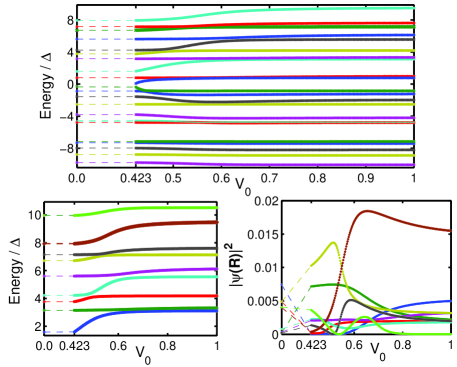
Figure 1: (Color online) The evolution of the energy levels and wave functions as a function of coupling strength for a realization drawn from the GOE (calculated using infinite-$U$ SBMFT). (a) Energy levels near the Fermi energy $\mu=0$ for coupling $V_{0}$ (from 0.423 to 1.0). (b) Zoom of a few levels above the Fermi energy. (c) The wave function amplitudes $|\psi({\bf R})|^{2}$ corresponding to the energy levels in (b) for an arbitrary position ${\bf R}\neq 0$. Parameters: band width $D=3.$, $E_{d}=-0.7$, $\Delta=0.0075$, and $T=0.005$.

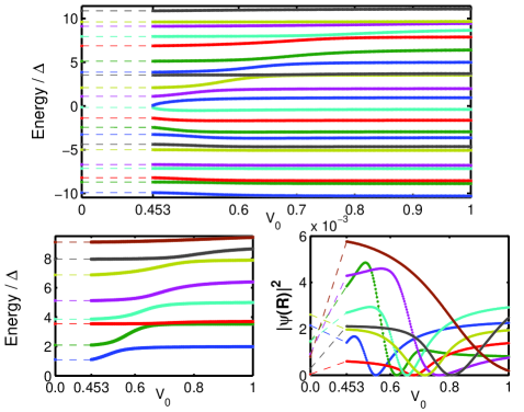
Figure 2: (Color online) The analog of Fig. 1 for the GUE; parameters are the same. Note that the variation is smoother for these GUE results than for the GOE in Fig. 1.

As an example of the output from this procedure, we show in Figs. 1 and 2, as a function of the strength of the coupling $V_{0}$, the one-body energy levels that result from a slave-boson mean field theory (SBMFT) treatment of the Anderson box for a particular realization of the box. As we discuss in more detail below (see section IV.2), a non-trivial solution of the SBMFT equations exists only for $J_{K}$ above some critical value $J^{c}_{K}$, or equivalently [see Eq. (6)] for $V_{0}$ larger than a threshold $V^{c}_{0}$. We thus show the non-interacting levels below that value and break the axis at that point [$V^{c}_{0}\simeq 0.423$ (GOE) and $V^{c}_{0}\simeq 0.453$ (GUE) for the realizations chosen]. Clearly, the levels do indeed shift substantially as a function of coupling strength; notice as well the additional level injected near the Fermi energy. The change in the levels occurs more sharply and for slightly smaller values of $V_{0}$ in the GOE case than for the GUE. Finally, we observe that, as one follows a level as a function of $V_{0}$, little change occurs after some point. The coupling strength $V_{0}$ at which levels reach their limiting value depends on the distance to the Fermi energy; it corresponds to the point where the Abrikosov-Suhl resonance becomes large enough to include the considered level. These limiting values of the energies are the SBMFT approximation to the single quasi-particle levels of the Nozières Fermi liquid theory.

II.5 Qualitative behavior

Before entering into the detailed quantitative analysis, we describe here some simple general properties of the mesoscopic Kondo problem within the SBMFT perspective.

We note first that the mean-field equations (II.4)-(24), have a trivial solution $\eta=0$ and $\xi=E_{d}$. This solution is actually the only one in the high temperature regime: the mesoscopic bath is effectively decoupled from the local magnetic impurity which can be considered a free spin-$1/2$. The onset of a solution $\eta\neq 0$ defines, in the mean field approach, the Kondo temperature $T_{\rm K}$.

Below $T_{\rm K}$, the self-consistent mean-field approach results in an effective one-particle problem, specifically a resonant level model with resonant energy $E_{d}\!+\!\mu\!-\!\xi$ and effective coupling $\eta V_{0}$. This resonance is interpreted as the Abrikosov-Suhl resonance characterizing the one-particle local energy spectrum of the Kondo problem below $T_{\rm K}$. The width of this resonance, $\Gamma(\eta)=\eta^{2}\Gamma_{0}$, vanishes for $T=T_{\rm K}$, and quickly reaches a value of order $T_{\rm K}$ when $T\ll T_{\rm K}$ (more detailed analysis is in Sec. III.2). Note that the mesoscopic Kondo problem differs from the bulk case: mesoscopic fluctuations may affect the large but finite number of energy levels that lie within the resonance.

The Anderson box is, however, a many-body problem. Its ground state cannot be described too naively in terms of one-body electronic wave functions, and more generally one should question the validity of the one particle description for each physical quantity under investigation. In this respect however, the configuration we consider, namely the low temperature regime of the Kondo box problem, is particularly favorable. Indeed, the line of argument developed by Nozières Nozières (1974) to show that the low temperature regime of the Kondo problem is a Fermi-liquid applies equally well in the mesoscopic case as in the bulk one for which it was originally devised. Therefore, as long as both the temperature $T$ and the mean level spacing $\Delta$ are much smaller than the Kondo temperature, we a priori expect the physics of the Kondo box to be described in terms of fermionic quasi-particles. The notions of one particle energies and wavefunction fluctuations in the strong interaction regime, which will be our main concern below, are therefore relevant. We take the point of view that, as in the bulk case Lee et al. (2006); Burdin (2009); Coleman (1983); Read et al. (1984), the mean field approach provides a good approximation for these quasi-particles in this low temperature regime, and therefore for the physical quantities derived from them Ullmo et al. . As we shall see furthermore, most of the fluctuation properties we shall investigate have universal features that makes them largely independent from possible corrections to this approximation (such as, for instance, corrections on the Kondo temperature), making the approach we are following particularly robust.

III Fluctuations of the mean field parameters

To begin our investigations of the low temperature properties of the mesoscopic Kondo problem within SBMFT, we consider the fluctuations of the mean field parameters $\eta$ and $\xi$ appearing in Eq. (12). We shall comment also on the degree to which these fluctuations are connected with those of the Kondo temperature $T_{\rm K}$ Kettemann (2004); Kaul et al. (2005); Bedrich et al. (2010).

III.1 Preliminary analysis

We start with a few basic comments about the eigenvalues $\{\lambda_{\kappa}-\mu\}$ and eigenstates $|\psi_{\kappa}\rangle$ ($\kappa=0,1,\cdots,N$) of the mean field Hamiltonian Eq. (12). Concerning the latter, we shall be interested in the two quantities,

$$u_{\kappa} \equiv |\langle f|\psi_{\kappa}\rangle|^{2}~{},$$ (25)

$$\theta_{\kappa} \equiv \langle 0|\psi_{\kappa}\rangle\langle\psi_{\kappa}|f\rangle\;.$$ (26)

$u_{\kappa}$ measures the overlap probability between the eigenstate $\kappa$ and the impurity state $|f\rangle$, and $\theta_{\kappa}$ the admixture of this eigensate with $|f\rangle$ and $|0\rangle=\sum_{i}\phi_{i}(0)|i\rangle$, the electron-bath state connected to the impurity. Note that $\theta_{\kappa}$ is a real quantity. In this section we use $\kappa=0$ to denote the additional resonant level added to the original system, and so in the limit $V_{0}\to 0$, one has $|\psi_{0}\rangle\to|f\rangle$ and $\lambda_{\kappa}\to\epsilon_{i=\kappa}$ ($\kappa=1,\ldots,N$).

Expressing the Green function of the mean field Hamiltonian as

$$\hat{G}(\lambda-\mu)=[\lambda-\mu-H_{\rm MF}]^{-1}=\sum_{\kappa=0}^{N}\frac{|\psi_{\kappa}\rangle\langle\psi_{\kappa}|}{\lambda-\lambda_{\kappa}}\;,$$ (27)

we can check that $(\lambda_{\kappa}-\mu)$ are the poles of the Green function $G_{ff}(z)=\langle f|\hat{G}(z)|f\rangle$. From Eq. (II.4) we have therefore immediately that the $\lambda_{\kappa}$ are the solutions of the equations

$$\frac{\Delta}{\pi}\sum_{i=1}^{N}\frac{x_{i}}{\lambda-\epsilon_{i}}=\frac{\lambda-\mathcal{E}_{0}(\xi)}{\Gamma(\eta)}\;,$$ (28)

where we have used the notation

$$\mathcal{E}_{0}(\xi) \equiv E_{d}+\mu-\xi$$

$$\Gamma(\eta) \equiv \eta^{2}\Gamma_{0}=\pi\rho_{0}\eta^{2}V_{0}^{2}$$ (29)

for the center and the width of the resonance, and $x_{i}\equiv N|\phi_{i}(0)|^{2}$ for the normalized wavefunction probability at ${\bf r}=0$. Note first that Eq. (28) implies that there is one and only one $\lambda_{\kappa}$ in each interval $[\epsilon_{i},\epsilon_{i+1}]$: the two sets of eigenvalues are interleaved and so certainly heavily correlated. Furthermore, $|\langle f|\psi_{\kappa}\rangle|^{2}$ are the corresponding residues, so again, from Eq. (II.4),

$$u_{\kappa}=\frac{1}{1+\displaystyle\frac{\Gamma(\eta)}{\pi}\sum_{i=1}^{N}\frac{x_{i}\Delta}{(\lambda_{\kappa}-\epsilon_{i})^{2}}}\;.$$ (30)

Eq. (28) is easily solved outside of the resonance, i.e. when $|\lambda-\mathcal{E}_{0}(\xi)|\gg\Gamma(\eta)$: in that case one contribution $i(\kappa)$ dominates the sum on the left hand side. [With our convention where $\kappa=0$ corresponds to the extra level added to the original system, we actually just have $i(\kappa)=\kappa$.] The solution for the fractional shift in the level, $\delta_{\kappa}\equiv(\lambda_{\kappa}-\epsilon_{i(\kappa)})/\Delta$ is then given by

$$\delta_{\kappa}\simeq\frac{\Gamma(\eta)}{\pi}\frac{x_{i(\kappa)}}{\lambda_{\kappa}-\mathcal{E}_{0}}\ll 1\;.$$ (31)

Eq. (30) and (31) then yield for the wave function intensity

$$u_{\kappa}\simeq\frac{\Gamma(\eta)}{\pi}\frac{x_{i(\kappa)}\Delta}{(\lambda_{\kappa}-\mathcal{E}_{0})^{2}}\ll\frac{\Delta}{\Gamma(\eta)}\;.$$ (32)

If the resonance is small [$\Gamma(\eta)\ll\Delta$], all states are accounted for in this way, except for $\lambda_{0}\simeq\mathcal{E}_{0}$ which is then such that $u_{\kappa=0}\simeq 1$.

If the resonance is large, $\Gamma(\eta)\gg\Delta$, the states within the resonance – those satisfying $|\lambda-\mathcal{E}_{0}(\xi)|\ll\Gamma(\eta)$ – must be treated differently. Because the left hand side of Eq. (28) can be neglected in this regime, these states have only a weak dependence on $\Gamma(\eta)$. The typical distance between a $\lambda_{\kappa}$ and the closest $\epsilon_{i}$ is then of order $\Delta$, and the corresponding wave functions participate approximately equally in the Kondo state,

$$u_{\kappa}\sim\Delta/\Gamma(\eta)\quad\mbox{[inside the resonance]}\;.$$ (33)

In a similar way, the admixture coefficient, $\theta_{\kappa}$, is the residue of $\langle 0|\hat{G}(z)|f\rangle=\sum_{i}\phi^{\star}(0)G_{if}(z)$ at the pole $z_{\kappa}=\lambda_{\kappa}-\mu$. Applying Eqs. (20) and (28), we thus immediately have

$$\theta_{\kappa}=u_{\kappa}\cdot\frac{1}{\eta V_{0}}\frac{\Gamma(\eta)\Delta}{\pi}\sum_{i}\frac{x_{i}}{\lambda_{\kappa}-\epsilon_{i}}=u_{\kappa}\cdot\frac{\lambda_{\kappa}-\mathcal{E}_{0}}{\eta V_{0}}\;.$$ (34)

Assuming the resonance is large [$\Gamma(\eta)\gg\Delta$], and inserting the limiting behaviors of $u_{\kappa}$ Eqs. (32)-(33), we obtain

$$\theta_{\kappa}\simeq\theta^{\rm out}_{\kappa} = \frac{x_{i(\kappa)}}{\pi}\frac{\Delta}{\eta V_{0}}\frac{\Gamma(\eta)}{\lambda_{k}-\mathcal{E}_{0}}\quad[|\lambda_{\kappa}\!-\!\mathcal{E}_{0}|\gg\Gamma]~{},$$ (35)

$$\theta_{\kappa} \sim \frac{\Delta}{\eta V_{0}}\frac{\lambda_{k}-\mathcal{E}_{0}}{\Gamma(\eta)}\qquad[|\lambda_{\kappa}\!-\!\mathcal{E}_{0}|\ll\Gamma]\;.$$ (36)

III.2 Formation of the resonance

Before considering the fluctuations of the mean field parameters $\eta$ and $\xi$ , let us first discuss the physical mechanisms that determine their value. While this discussion is not specific to the mesoscopic Kondo problem, it is useful to review it briefly before addressing the mesoscopic aspects.

The self-consistent equations (13)-(14) or (II.4)-(24) can be written as (performing the summation over Matsubara frequencies in the standard way Fetter and Walecka (1971) in the latter case),

$$2V_{0}\sum_{\kappa=0}^{N}(f_{\kappa}\!-\!\frac{1}{2})\,\theta_{\kappa} = \eta\xi\;,$$ (37)

$$n_{f}=\sum_{\kappa=0}^{N}f_{\kappa}u_{\kappa} = \frac{1-\eta^{2}}{2}\;,$$ (38)

where $f_{\kappa}=f(\lambda_{\kappa}\!-\!\mu)=[1+\exp((\lambda_{\kappa}\!-\!\mu)/T)]^{-1}$ is the Fermi occupation number. One furthermore has the sum rules $\sum_{\kappa}u_{\kappa}=\langle f|f\rangle=1$ and $\sum_{\kappa}\theta_{\kappa}=\langle 0|f\rangle=0$ [the latter has been used to generate the 1/2 in (37)].

As mentioned in Sec. II.5, the trivial solution of these mean-field equations ($\eta\!=\!0,\xi\!=\!E_{d}$) is the only one in the high temperature regime. The Kondo temperature $T_{\rm K}$ is defined, in the mean field approach, as the highest temperature for which a $\eta\neq 0$ solution occurs. One obtains an equation for $T_{\rm K}$ by requiring that the non-trivial solution of the mean-field equations continuously vanishes, $\eta\to 0^{+}$, in which case $\lambda_{\kappa=0}\to\mathcal{E}_{0}(\xi)$, $u_{\kappa=0}\to 1$, and $u_{\kappa\neq 0}\to 0$. Eq. (38) then reduces to $f(\mathcal{E}_{0}(\xi)-\mu)=1/2$, implying $\mathcal{E}_{0}(\xi)=\mu$ and so $\xi=E_{d}$. Using Eq. (35) to simplify Eq. (37) then gives the mesoscopic version Bedrich et al. (2010) of the Nagaoka-Suhl equation Nagaoka (1965); Suhl (1965)

$$\frac{E_{d}}{V_{0}^{2}}=\sum_{i=1}^{N}\frac{|\phi_{i}(0)|^{2}}{\epsilon_{i}-\mu}\tanh{[(\epsilon_{i}-\mu)/2T_{\rm K}]}\;.$$ (39)

The same equation for $T_{\rm K}$ was obtained from a one-loop perturbative renormalization group treatment Zaránd and Udvardi (1996); Kaul et al. (2005).

In the bulk limit ($N\to\infty$ and no fluctuations) and for $\mu$ in the middle of the band, this gives $T_{\rm K}^{\rm bulk}=a_{K}(D/2)e^{-1/J_{K}\rho_{0}}$ for the Kondo temperature, with $a_{K}\simeq 1.13\cdot\cdot$ as shown in Appendix A. Unless explicitly specified, we will always assume this quantity is large compared to the mean level spacing. In this case, the fluctuations of the Kondo temperature for chaotic dynamics described by the random matrix model in Sec. II.2 has been analyzed in Refs. Kaul et al., 2005-Kettemann, 2004 and more recently using SBMFT in Ref. Bedrich et al., 2010. The main result is that $\delta T_{\rm K}$, the fluctuation of the Kondo temperature around the bulk Kondo temperature, scales as

$$\overline{(\delta T_{\rm K})^{2}}\sim T_{\rm K}^{\rm bulk}\Delta\;.$$ (40)

Now consider what happens as $T$ decreases further below $T_{\rm K}$. Dividing Eq. (37) by $\eta V_{0}$, we can write it as

$$\frac{\xi}{V_{0}^{2}}=\sum_{\kappa=0}^{N}r_{\kappa}\frac{|\phi_{i(\kappa)}(0)|^{2}}{\lambda_{\kappa}-\mathcal{E}_{0}}\tanh{[(\lambda_{\kappa}-\mu)/2T]}\;,$$ (41)

where $r_{\kappa}={\theta_{\kappa}}/{\theta^{\rm out}_{\kappa}}$ is one outside the resonance and scales as $(\lambda_{\kappa}-\mathcal{E}_{0})^{2}/\Gamma(\eta)^{2}$ within the resonance [see Eqs. (35)-(36)]. Eq. (41) has a structure very similar to the equation for $T_{\rm K}$, Eq. (39). Indeed, $\xi$ might not be strictly equal to $E_{d}$ [and thus $\mathcal{E}_{0}(\xi)$ might differ slightly from $\mu$] but its scale will remain the same. Then outside the resonance, $\lambda_{\kappa}\simeq\epsilon_{i(\kappa)}$ and $r_{\kappa}\simeq 1$. The main difference in the expression for $\xi$ is that the logarithmic divergence associated with the summation of $1/(\lambda_{\kappa}-\mathcal{E}_{0})$ is cutoff not only by the temperature factor $\tanh{[(\lambda_{\kappa}-\mu)/2T]}$ at the scale $T$, but also by the ratio $r_{\kappa}$ at the scale $\Gamma(\eta)$. As $T$ becomes significantly smaller than $T_{\rm K}$, the temperature cutoff becomes inoperative. This implies in particular that $\Gamma(\eta)$ will rather quickly switch from 0 to its zero temperature limit when $T$ goes below $T_{\rm K}$. We shall in the following not consider the temperature dependence of $\Gamma(\eta)$ but rather focus on its low temperature limit.

We see, then, that both $T_{\rm K}$ and $\Gamma(\eta)$ represent physically the scale at which the logarithmic divergence of $\sum_{i}|\phi_{i}(0)|^{2}/(\epsilon_{i}-\mu)$ should be cut to keep this sum equal to $E_{d}/V_{0}^{2}$. Thus, as long as we are only interested in energy scales, we can write that for $T\ll T_{\rm K}$,

$$\Gamma(\eta)\sim T_{\rm K}\;.$$ (42)

The energy dependence of the cutoff $r_{\kappa}$ within the resonance, however, differs slightly from that of $\tanh{[(\lambda_{\kappa}-\mu)/2T_{\rm K}]}$ below $T_{\rm K}$. As an exponentiation is involved, the prefactors of $\Gamma(\eta)$ and $T_{\rm K}$ somewhat differ; a discussion of the ratio $\Gamma(\eta)/T_{\rm K}$ for the bulk case is given in Appendix A.

At low temperature, $\eta$ is fixed in such a way that $\Gamma(\eta)$ is of the scale of the Kondo temperature. The condition Eq. (38) then fixes $\xi$, which governs the center of the resonance $\mathcal{E}_{0}(\xi)$ so a proportion $(1-\eta^{2})/2$ of the resonance is below the Fermi energy $\mu$. In the Kondo regime when $n_{f}\simeq 1/2$, $\mathcal{E}_{0}(\xi)$ will therefore remain near $\mu$. In the mixed valence regime $\mathcal{E}_{0}(\xi)$ will float a bit above $\mu$ for a distance $-\delta\xi=E_{d}-\xi$ which scales as $\delta\xi\sim\eta^{2}\Gamma_{0}\lesssim E_{d}$. The order of magnitude of $\xi$ remains thus $E_{d}$ [as we have assumed above when discussing Eq. (41)].

III.3 Fluctuations scale of the mean field parameters

With this physical picture of how the mean field parameters $\eta$ and $\xi$ are fixed, it is now relatively straightforward to evaluate the scale of their fluctuations. For simplicity, we assume $T=0$ so the mean-field equations become

$$I(\eta,\xi) \equiv \pi\sum_{\kappa=0}^{N}{\rm sgn}(\lambda_{\kappa}\!-\!\mu)\frac{(\lambda_{\kappa}\!-\!\mathcal{E}_{0})}{\Gamma(\eta)}\,u_{\kappa}=\frac{\pi\xi}{\Gamma_{0}}\quad~{},$$ (43)

$$J(\eta,\xi) \equiv \sum_{\lambda_{\kappa}<\mu}u_{\kappa}=\frac{1-\eta^{2}}{2}\;.$$ (44)

The discussion below generalizes easily to finite $T$ as long as it is much smaller than $T_{\rm K}$.

The average values of $I(\eta,\xi)$ and $J(\eta,\xi)$ are well approximated by their “bulk-value” analogues $I^{\rm bulk}(\eta,\xi)$ and $J^{\rm bulk}(\eta,\xi)$, obtained with the same global parameters but with the fluctuating wave-function probabilities $x_{i}$ replaced by $1$ and the spacing between successive levels taken constant, $\epsilon_{i+1}\!-\epsilon_{i}\equiv\Delta$. We furthermore denote by $(\bar{\eta},\bar{\xi})$ the solution of Eqs. (43)-(44) with $I(\eta,\xi)$ and $J(\eta,\xi)$ replaced by their bulk approximation, by $\delta\eta\equiv\eta-\bar{\eta}$ and $\delta\xi\equiv\xi\!-\!\bar{\xi}$ the fluctuating part of the mean field parameters, and by $\delta I(\eta,\xi)\equiv I(\eta,\xi)\!-\!I(\eta,\xi)^{\rm bulk}$ and $\delta J(\eta,\xi)\equiv J(\eta,\xi)\!-\!J(\eta,\xi)^{\rm bulk}$ the fluctuating parts of the sums appearing in Eqs. (43)-(44).

We start by discussing the Kondo limit $T_{\rm K}\ll\Gamma_{0}$, in which case $\bar{\eta}\ll 1$, $\bar{\xi}\!-\!E_{d}\ll\Gamma$, and $\bar{\Gamma}\equiv\Gamma(\bar{\eta})=(D/2)\exp(-1/J_{K}\rho_{0})$. A calculation in Appendix A shows

$$I^{\rm bulk}(\eta,\xi) = 2\ln\left(\frac{D}{2\Gamma(\eta)}\right)+O(\eta^{4})~{},$$ (45)

$$J^{\rm bulk}(\eta,\xi) = \frac{1}{2}+\frac{1}{\pi}\frac{\xi\!-\!E_{d}}{\Gamma(\eta)}+O(\eta^{4})\;.$$ (46)

Furthermore, as we shall be able to verify below, the leading contribution to the fluctuations of $\eta$ and $\xi$ can be taken independently of each other (i.e. the fluctuations of $\xi$ can be computed assuming $\eta$ constant, and reciprocally).

Subtracting its bulk value from Eq. (44), we have $J(\eta,\xi)-J^{\rm bulk}(\bar{\eta},\bar{\xi})\simeq-\bar{\eta}\delta\eta$, and thus, by definition of $\delta J(\eta,\xi)$,

$$J^{\rm bulk}(\bar{\eta}+\delta\eta,\bar{\xi}+\delta\xi)-J^{\rm bulk}(\bar{\eta},\bar{\xi})=-\delta J(\eta,\xi)-\bar{\eta}\delta\eta\;.$$

If the fluctuations of $\xi$ and $\eta$ are small, we can furthermore approximate $\delta J(\eta,\xi)$ by $\delta J(\bar{\eta},\bar{\xi})$. We thus have

$$\frac{1}{\pi}\frac{\delta\xi}{\Gamma(\bar{\eta})}=-\delta J(\bar{\eta},\bar{\xi})+\frac{2}{\pi}\frac{(\bar{\xi}-E_{d})}{\Gamma(\bar{\eta})}\frac{\delta\eta}{\bar{\eta}}-\bar{\eta}^{2}\frac{\delta\eta}{\bar{\eta}}\;.$$ (47)

The two last terms on the right-hand-side of Eq. (47) are proportional to $\bar{\eta}^{2}$ [e.g. see Eq. (100) for the second-to-last term] and so are negligible in the Kondo regime. Computing the variance $\overline{(\delta\xi)^{2}}$ therefore amounts, up to the constant factor $\pi\Gamma(\bar{\eta})$, to computing the variance of $\delta J(\bar{\eta},\bar{\xi})$.

Now, for $\Gamma(\eta)\gg\Delta$, we have $u_{\kappa}=\tilde{u}_{\kappa}[\pi\Delta/\Gamma(\eta)]$, where

$$\tilde{u}_{\kappa}\equiv\left[\sum_{i=1}^{N}\frac{x_{i}\Delta^{2}}{(\lambda_{\kappa}-\epsilon_{i})^{2}}\right]^{-1}$$ (48)

is a dimensionless quantity which for $(\lambda_{\kappa}\!-\!\mathcal{E}_{0})\ll\Gamma(\eta)$ is essentially independent of $\xi$, $\Gamma(\eta)$, or the other parameters of the model. Within the resonance, and for our random matrix model, we therefore can take the $\tilde{u}_{\kappa}$ to have identical distributions (independent of $\kappa$) characterized by a variance $\sigma^{2}_{u}$ of order one. Neglecting the correlations between the $\tilde{u}_{\kappa}$, and treating the $\kappa$ at the edge of the resonance as if they were well within it (which is obviously incorrect but should just affect prefactors that we are in any case not computing), we have

$$\overline{(\delta J)^{2}}\sim\sum_{-\Gamma<(\lambda_{\kappa}-\mu)<0}\sigma_{u}^{2}\frac{\pi^{2}\Delta^{2}}{\bar{\Gamma}^{2}}\sim(\pi\sigma_{u})^{2}\frac{\Delta}{\bar{\Gamma}}\;.$$ (49)

Inserting this into Eq. (47), we finally get

$$\overline{(\delta\xi)^{2}}\sim\bar{\Gamma}\Delta\sim T_{\rm K}\Delta\;.$$ (50)

With regard to the limits of validity of this estimate, note that our random matrix model (Sec. II.2) assumes implicitly that the Thouless energy $E_{\rm Th}$ is infinite, and more specifically that $E_{\rm Th}\gg T^{\rm bulk}_{K}$. For a chaotic ballistic system with $E_{\rm Th}\ll T^{\rm bulk}_{K}$, the $\tilde{u}_{\kappa}$ are independent only in an interval of size $E_{\rm Th}$; thus, Eq. (50) should be replaced by $\overline{(\delta\xi)^{2}}\sim E_{\rm Th}\Delta$.

For the fluctuations of $\eta$, we proceed in a similar way, subtracting Eq. (43) from its bulk analog and assuming small fluctuations, and so find

$$\frac{\delta\eta}{\bar{\eta}}=\frac{\delta\Gamma}{2\bar{\Gamma}}=\frac{1}{4}\left[\delta I(\bar{\eta},\bar{\xi})-\frac{\pi\delta\xi}{\Gamma_{0}}\right]\;.$$ (51)

Here, however, it is necessary to split the sum over states in Eq. (43) into two parts: $I=I^{\rm in}+I^{\rm out}$ where $I^{\rm in}$ and $I^{\rm out}$ are defined in the same way as $I$ but over an energy range corresponding, respectively, to the inside and outside of the resonance. One has $I^{\rm out}(\eta,\xi)\gg I^{\rm in}(\eta,\xi)$ since the former contains the logarithmic divergence. However, the fluctuations of the two quantities are of the same order [basically because when considering the variance, and thus squared quantities, one transforms a diverging sum $\sum_{\kappa}(\lambda_{\kappa}-\mathcal{E}_{0})^{-1}$ into a converging one $\sum_{\kappa}(\lambda_{\kappa}-\mathcal{E}_{0})^{-2}$]. Indeed, the sum $I^{\rm out}(\eta,\xi)$ is, up to sub-leading corrections, the same as the one entering into the definition of $T_{\rm K}$. Its fluctuations have been evaluated in Refs.  Kaul et al., 2005-Kettemann, 2004, leading to

$$\overline{(\delta I^{\rm out})^{2}}\sim\frac{\Delta}{T_{\rm K}^{\rm bulk}}\;,$$ (52)

which is consistent with Eq. (40). The variance of $\delta I^{\rm in}$ can, on the other hand, be evaluated following the same route as for $\delta J$, yielding

$$\overline{(\delta I^{\rm in})^{2}}\sim 2\sum_{0<(\lambda_{\kappa}-\mu)<\Gamma}\frac{\sigma_{u}^{2}}{(\bar{\Gamma}/\pi\Delta)^{2}}\frac{\pi^{2}}{\Gamma(\eta)^{2}}(\lambda_{\kappa}-\mathcal{E}_{0})^{2}\sim\frac{\Delta}{\bar{\Gamma}}\;.$$ (53)

This shows, then, that the two contributions $\overline{(\delta I^{\rm in})^{2}}$ and $\overline{(\delta I^{\rm out})^{2}}$ scale in the same way.

For the final contribution—the last term on the r.h.s. of Eq. (51)—Eq. (50) implies

$$\frac{\pi\overline{(\delta\xi)^{2}}}{\Gamma_{0}}\sim\eta^{2}\frac{\Delta}{\bar{\Gamma}}\;,$$ (54)

which is proportional to ${\Delta}/{\bar{\Gamma}}$ as for the first two contributions, but the extra smallness factor $\eta^{2}$ makes it negligible in the Kondo limit. Gathering everything together, we therefore obtain

$$\frac{\overline{(\delta\eta)^{2}}}{\bar{\eta}^{2}}=\frac{\langle(\delta\Gamma)^{2}\rangle}{4\bar{\Gamma}^{2}}\sim\frac{\Delta}{\bar{\Gamma}}\;.$$ (55)

[If $E_{\rm Th}\ll\Gamma(\eta)$, $\overline{(\delta\xi)^{2}}$ and $\overline{(\delta I^{\rm in})^{2}}$ are reduced by a factor $(E_{\rm Th}/\bar{\Gamma})$, but not $\overline{(\delta I^{\rm out})^{2}}$; thus, Eq. (55) remains unchanged.]

Turning to the mixed-valence regime by releasing the constraint $\eta\ll 1$, we see that $\pi\overline{(\delta\xi)^{2}}/\Gamma_{0}$ becomes comparable in size to the other contributions to $\overline{(\delta\eta)^{2}}$ and has the same parametric dependence. Furthermore, taking the derivative $\partial J^{\rm bulk}/\partial\xi$ [see Eq. (99)] implies that the left hand side of (47) should be multiplied by a factor $\bar{\Gamma}/(\bar{\Gamma}^{2}-(\bar{\xi}-\mathcal{E}_{0})^{2})$, which, however, does not change the scaling of $\overline{(\delta\eta)^{2}}$. In the same way, using Eq. (55) the two last terms on the right hand side of Eq. (47), which are proportional to $\delta\eta/\bar{\eta}$, give a contribution $\sim\eta^{4}\bar{\Gamma}\Delta$ to $\overline{(\delta\xi)^{2}}$, as well as the term $(\bar{\xi}-E_{d})\delta\xi/(\bar{\Gamma}^{2}-(\bar{\xi}-\mathcal{E}_{0})^{2})$ that should be added to the the left hand side of Eq. (51) from $\partial I^{\rm bulk}/\partial\xi$ [see Eq. (98)]. Those are negligible in the Kondo regime, but are of the same size and with the same scaling as the contribution due to $\delta J$ in the mixed-valence regime. We find, then, that the fluctuations of the mean field parameters scale with system size in the same way in both the Kondo and mixed-valence regimes: the variance of both $\xi$ and $\eta$ is proportional to $\Delta$.

III.4 Numerical investigations

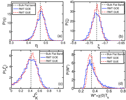
Figure 3: (Color online) The distribution of the mean field parameters, critical coupling, and effective Wilson number from the SBMFT calculation for both GOE (blue solid line) and GUE (red dash-dotted line). (a) $\eta$, (b) $\xi$, (c) critical coupling $J_{K}^{c}$, and (d) the effective Wilson number $W^{*}=T_{\rm K}\chi_{0}(0)$. The vertical black dashed lines mark the values for the corresponding bulk flat-band system. The following parameters were used: band width $D=3$, $E_{d}=-0.7$, $V_{0}=0.6$, and $T=0.005$. The mean level spacing is $\Delta=0.01$, and the Kondo temperature in the bulk limit is $T_{\rm K}^{\rm bulk}\simeq 0.092$.

To illustrate the previous discussion, we have computed numerically the self-consistent parameters $\eta$ and $\xi$ for a large number of realizations of our random matrix ensemble at various values of the parameters defining the Anderson box model (always within our regime of interest, $T\!<\!\Delta\!\ll\!T_{\rm K}$, except when explicitly specified). Fig. 3 shows the distributions of $\eta$ and $\xi$ for a choice of parameters such that $T_{\rm K}^{\rm bulk}/\Gamma_{0}\simeq 0.24$ (close to but not in the mixed valence regime). We see that these distributions are approximately Gaussian and centered on their values for the bulk flat-band case, though note the slightly non-Gaussian tail on the left side in both cases. The distributions for the GOE and GUE are qualitatively similar, with those for the GUE being, as expected, slightly narrower. As anticipated, the fluctuation of these mean parameters is small: the root-mean-square variation is less than 5% of the mean. Fig. 4 further shows how the variance of $\eta$ and $\xi$ varies with the parameters of the model, confirming the behavior in Eqs. (50) and (55).

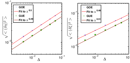
Figure 4: (Color online) Variance of the mean field parameters $\eta$ (left panel) and $\xi$ (right) as the size of the system is changed. The change in system size is quantified through the mean level separation $\Delta$. As expected, the fluctuations are smaller in the GUE compared to the GOE, and the dependence of the variance of the fluctuations on $\Delta$ is nearly linear. Here, we use $D=3$, $E_{d}=-0.7$, and $V_{0}=0.8$.

IV Other global physical properties

Beyond $\eta$ and $\xi$ themselves, several interesting global properties of the system follow directly from the solution of the mean-field problem. We briefly discuss two of them here.

IV.1 Wilson number: Comparing $T_{\rm K}$ and the ground state properties

The “Wilson number” is an important quantity in Kondo physics: it compares $T_{\rm K}$ with the energy scale contained in the ground state magnetic susceptibility. It is defined as $W^{*}\equiv T_{\rm K}\,\chi_{0}({T\!\rightarrow\!0})$, where $\chi_{0}(T)\equiv\int_{0}^{1/T}\langle S^{z}(\tau)S^{z}(0)\rangle d\tau$ is the static susceptibility. $W^{*}$ is thus the ratio between the characteristic high temperature scale $T_{\rm K}$ and the characteristic low temperature scale $T_{0}=1/\chi_{0}(T=0)$ of the strong-coupling regime Burdin (2009).

In the bulk Kondo problem, there is only one scale, of course, and so the Wilson number has a fixed value Hewson (1993), namely $0.4128$ (approximated as $0.349$ in the SBMFT). For our mesoscopic Anderson box on the other hand, this will be a fluctuating quantity that has to be computed for each realization of the mesoscopic electron bath. Computing $T_{\rm K}$ according to Eq. (39) and expressing the static susceptibility as $\chi_{0}(T)=T\sum_{n=-\infty}^{+\infty}G_{ff}(i\omega_{n})G_{ff}(-i\omega_{n})$ with $G_{ff}(i\omega_{n})$ given by Eq. (II.4), we obtain the distribution of the Wilson number shown in Fig. 3(d). Note the unusual non-Gaussian form of the distribution, with the long tail for large $W^{*}$. As a result, the peak of the distribution is slightly smaller than the bulk flat-band value. The magnitude of the fluctuations in $W^{*}$ is modest for our choice of parameters (about 30%) but considerably larger than the magnitude of the fluctuations of the mean field parameters in Fig. 3(a)-(b).

IV.2 Critical Kondo coupling

Another interesting global quantity is the critical Kondo coupling $J_{K}^{c}[\{\epsilon_{i}\},\{|\phi_{i}(0)|^{2}\}]$ defined for a given realization of the electron bath by

$$\frac{1}{2J_{K}^{c}}\equiv\sum_{i=1}^{N}\frac{|\phi_{i}(0)|^{2}}{|\epsilon_{i}-\mu|}\;.$$ (56)

Here, exceptionally, we move away from the regime $T_{\rm K}^{\rm bulk}\gg\Delta$. The discreetness of the spectrum is what is making convergent the sum in the above expression, and thus $J_{K}^{c}$ can be defined only because of the finite size of the electron bath.

Comparing with Eq. (39), we see that in the SBMFT approximation ${J_{K}^{c}}$ is the realization-dependent value of the Kondo coupling $J_{K}$ [defined in Eq. (6)] such that $T_{\rm K}=0$ if $J_{K}<J_{K}^{c}$ and $T_{\rm K}$ is non-zero if $J_{K}>J_{K}^{c}$. Note that the possibility of vanishing the Kondo temperature $T_{K}$ has been discussed in the framework of disordered bulk systems Kettemann (2004); Kettemann and Mucciolo (2006, 2007); Zhuravlev et al. (2007); Miranda and Dobrosavljevic̀ (2001); Cornaglia et al. (2006). Fig. 3(c) shows the distribution of this critical coupling for a mesoscopic Anderson box. Note the non-Gaussian form of the distribution and the similarity between the GOE and GUE results. Remarkably the distribution functions do not vanish at $J_{K}^{c}=0$, indicating that there exist realizations for which the Kondo screening occurs for any coupling $V_{0}$ and impurity level $E_{d}$. Indeed, as pointed out in Ref. Bedrich et al., 2010, a small $J_{K}^{c}$ corresponds to a situation in which the chemical potential $\mu$ lies very close to some level $\epsilon_{i}$, which then dominates the sum in (56). If $\mu$ exactly coincides with some $\epsilon_{i}$, $J_{K}^{c}=0$: the large dot contains an odd number of electrons on average so the impurity can always form a singlet with the large dot Kaul et al. (2006).

V Spectral fluctuations

The mean field approach maps the Kondo problem at low temperatures into a resonant level problem, Eq. (12), with two realization specific parameters: the energy of the resonant level [$\mathcal{E}_{0}(\xi)$, taking $\mu=0$ as the energy reference] and the strength of the coupling to it. We have seen, however, that in the limit $T_{\rm K}\gg\Delta$ [or equivalently $\Gamma(\eta)\gg\Delta$] the scale of the fluctuations of these parameters both go to zero as $\sqrt{\Delta/\bar{\Gamma}}$. Furthermore, as long as $|\lambda_{\kappa}-\mathcal{E}_{0}|\ll\Gamma(\eta)$, the $\lambda_{\kappa}$ and corresponding $|\psi_{\kappa}\rangle$ are relatively insensitive to $\Gamma$ and $\mathcal{E}_{0}$ and thus to their fluctuations. We consider, therefore, in a first stage the fluctuations implied by the resonant level model (RLM) with fixed parameters, and then come back later to consider how the fluctuations of the parameters modify the results.

For the analysis in this section and the next, it is convenient to rewrite the resonant level model (RLM) as

$$H_{\rm RLM}\!=\!\sum_{i=1}^{N}\epsilon_{i}|i\rangle\langle i|+\epsilon_{0}|f\rangle\langle f|+v\sum_{i=1}^{N}[\sqrt{N}\phi_{i}(0)|i\rangle\langle f|+{\rm h.c.}].$$ (57)

Here, $|f\rangle$ is the bare resonant level state with energy $\epsilon_{0}$, and the $|i\rangle$ for $i\geq 1$ are the bare (unperturbed) states of the reservoir with wave functions $\phi_{i}({\bf r})$. The eigenstates of $H_{\rm RLM}$ (perturbed states) are, as before, $|\psi_{\kappa}\rangle$ for $\kappa=0,\cdots,N$ with corresponding eigenvalues $\{\lambda_{\kappa}\}$. Finally, the coupling strength is taken to scale with system size as $v\propto 1/\sqrt{N}$ so the large $N$ limit in the random matrix model can be conveniently taken. The corresponding width of the resonant level is $\Gamma\equiv\pi\rho_{0}Nv^{2}$.

We use two complementary ways of viewing the RLM. First, as a microscopic model in its own right, albeit non-interacting, one has $v=V_{0}/\sqrt{N}$ where $V_{0}$ is the hopping matrix element from the resonant level to the ${\bf r}=0$ site in the reservoir as in Eq. (3). In this case the width of the level is simply $\Gamma=\Gamma_{0}$, and $\epsilon_{0}$ is just a parameter of the model. Second, if one views the RLM as the result of an SBMFT approach in which the fluctuations of the mean field parameters are neglected, one has $v=\bar{\eta}V_{0}/\sqrt{N}$, in which case $\Gamma=\Gamma(\bar{\eta})=\bar{\Gamma}$, and $\epsilon_{0}=\mathcal{E}_{0}(\bar{\xi})$. We stress that in both views, $\epsilon_{0}$ and the $\epsilon_{i}$’s ($1\leq i\leq N$) are, in spite of the similarity in the notations, different objects in terms of the statistical ensemble considered: $\epsilon_{0}$ is a fixed parameter, when the $\epsilon_{i}$’s are random variables distributed according to Eq. (7).

V.1 Joint Distribution Function

To characterize the correlations between the unperturbed energy levels and the perturbed levels, the basic quantity needed is the joint distribution function $P(\{\epsilon_{i}\},\{\lambda_{\kappa}\})$. As seen in Sec. III.1, the RLM eigenvalues $\lambda_{\kappa}$ are related to the unperturbed energies through Eq. (28), which we rewrite as

$$\sum_{i=1}^{N}\frac{x_{i}}{\lambda_{\kappa}-\epsilon_{i}}=\frac{\lambda_{\kappa}-\epsilon_{0}}{v^{2}},$$ (58)

remembering that $x_{i}\equiv N|\phi_{i}(0)|^{2}$. Explicitly writing out the “interleaving” constraints, we obtain

$$\epsilon_{i}\leq \lambda_{i} \leq\epsilon_{i+1},\qquad i=1,\cdots,N-1$$

$$\lambda_{0} <\epsilon_{1}$$

$$\lambda_{N} >\epsilon_{N}\;.$$

(Note we slightly change the way we index the levels $\lambda_{i}$ with respect to section III.) There is furthermore an additional constraint on the sum of the eigenvalues

$$\mathcal{D}\equiv\sum_{i=0}^{N}\epsilon_{i}-\sum_{\kappa=0}^{N}\lambda_{\kappa}=0\;,$$ (60)

a proof of which is given in Appendix B.

Since we know the joint distribution of the $\epsilon_{i}$ and $|\phi_{i}(0)|^{2}$, we now want to use relation (58) to convert from the eigenfunctions to the $\lambda_{\kappa}$. A slight complication here is that there is one more level $\lambda_{\kappa}$ than wavefunction probabilities $|\phi_{i}(0)|^{2}$ (which is why a constraint such as Eq. (60) needs to appear). It is therefore convenient to include an additional “unperturbed” level at energy $\epsilon_{0}$ associated with a wave-function probability $x_{0}$, and to extend the summation in the left hand side of Eq. (58) to $i=0$. Assuming then that $x_{0}$ has a probability one to be zero [i.e. that $P(x_{0})=\delta(x_{0})$], one recovers the original problem.

In terms of the Jacobian for this variable transformation, the desired joint distribution then can be written as

$$P_{\beta}(\{\epsilon_{i}\},\{\lambda_{\kappa}\})=P_{\beta}(\{\epsilon_{i}\})\;\delta(x_{0})\;\prod_{i=1}^{N}p_{\beta}(x_{i})\;\bigg{\arrowvert}\det\left[\frac{\partial x_{i}}{\partial\lambda_{j}}\right]\bigg{\arrowvert}$$ (61)

where $P_{\beta}(\{\epsilon_{i}\})$ and $p_{\beta}(x_{i})$ are given in Eqs. (7) and (8). (We shall not assume in this subsection that the spectrum $\{\epsilon_{i}\}$ has been unfolded.) In order to find the Jacobian, we first find $x_{i}$ explicitly. Since Eq. (58) is linear in $x_{i}$, inverting the Cauchy matrix $a_{\kappa i}=1/(\lambda_{\kappa}-\epsilon_{i})$ yields

$$x_{i}=\sum_{\kappa}b_{i\kappa}\frac{\lambda_{\kappa}-\epsilon_{0}}{v^{2}}~{},$$ (62)

where Schechter (1959)

$$b_{i\kappa} = \frac{1}{\epsilon_{i}-\lambda_{\kappa}}\frac{A(\epsilon_{i})}{B^{{}^{\prime}}(\epsilon_{i})}\frac{B(\lambda_{\kappa})}{A^{{}^{\prime}}(\lambda_{\kappa})}~{},$$

$$A(z) = \prod_{\kappa=0}^{N}(z-\lambda_{\kappa}),\qquad B(z)=\prod_{i=0}^{N}(z-\epsilon_{i})\;.$$ (63)

This expression can be simplified by using the residue theorem twice. First, note that

$$x_{i} = -\frac{1}{v^{2}}\bigg{(}\frac{1}{2\pi i}\oint\frac{(z-\epsilon_{0})B(z)}{(z-\epsilon_{i})A(z)}dz\bigg{)}\frac{A(\epsilon_{i})}{B^{{}^{\prime}}(\epsilon_{i})}\;.$$ (64)

Second, the identity $\oint\prod_{i}(z-a_{i})/\prod_{i}(z-b_{i})dz=2\pi i\sum_{i}(b_{i}-a_{i})$ implies

$$x_{i}=\frac{1}{v^{2}}\left(\epsilon_{i}-\epsilon_{0}+\mathcal{D}\right)\frac{\prod_{\kappa=0}^{N}(\lambda_{\kappa}-\epsilon_{i})}{\prod_{i\neq j}(\epsilon_{j}-\epsilon_{i})}\;.$$ (65)

For $i=0$, this reads

$$x_{0}=\frac{1}{v^{2}}\mathcal{D}\cdot\frac{\prod_{\kappa=0}^{N}(\lambda_{\kappa}-\epsilon_{0})}{\prod_{j=1}^{N}(\epsilon_{j}-\epsilon_{0})}\;,$$ (66)

and thus $x_{0}\neq 0$ implies that the $\lambda_{\kappa}$ cannot coincide with $\epsilon_{0}$, leading then to

$$\delta(x_{0})=\frac{v^{2}\prod_{j=1}^{N}(\epsilon_{j}-\epsilon_{0})}{\prod_{\kappa=0}^{N}(\lambda_{\kappa}-\epsilon_{0})}\cdot\delta(\mathcal{D})\;.$$ (67)

The factor $\delta(x_{0})$ in Eq. (61) therefore imposes the constraint (60) that we know should hold.

Now note that $\partial x_{i}/\partial\lambda_{\kappa}$ is itself a Cauchy-like matrix $\partial x_{i}/\partial\lambda_{\kappa}=r_{i}s_{\kappa}/(\lambda_{\kappa}-\epsilon_{i})$ where

$$r_{i}=\frac{1}{v^{2}}\frac{\prod_{\kappa}(\lambda_{\kappa}-\epsilon_{i})}{\prod_{\kappa\neq i}(\epsilon_{\kappa}-\epsilon_{i})}\quad\text{and}\quad s_{\kappa}=\lambda_{\kappa}-\epsilon_{0}+\mathcal{D}\;.$$ (68)

The Jacobian, then, is given by

$$\det\bigg{(}\frac{\partial x_{i}}{\partial\lambda_{\kappa}}\bigg{)} = \prod_{i=0}^{N}r_{i}\prod_{\kappa=0}^{N}s_{\kappa}\det\bigg{(}\frac{1}{\lambda_{\kappa}-\epsilon_{i}}\bigg{)}$$ (69)

$$= \frac{\prod_{\kappa}(\lambda_{\kappa}-\epsilon_{0}+\mathcal{D})}{v^{2N}}\frac{\prod_{j>i}(\lambda_{j}-\lambda_{i})}{\prod_{j>i}(\epsilon_{j}-\epsilon_{i})}\;.$$

From now on, since no further derivative will be taken, we can set $x_{0}$, and thus $\mathcal{D}$, to zero, and thus assume that the constraint (60) holds. The last ingredient we need in order to assemble the joint distribution function is $\sum_{i}x_{i}$:

$$\sum_{i}x_{i} = \frac{1}{v^{2}}\sum_{i}(\epsilon_{0}-\epsilon_{i})\frac{A(\epsilon_{i})}{B^{{}^{\prime}}(\epsilon_{i})}$$ (70)

$$= -\frac{1}{2\pi iv^{2}}\oint\frac{(z-\epsilon_{0})A(z)}{B(z)}dz$$

$$= -\frac{1}{2\pi iv^{2}}\oint\frac{\prod_{\kappa=0}^{N}(z-\lambda_{\kappa})}{\prod_{i=1}^{N}(z-\epsilon_{i})}dz\;.$$

The relation

$$\frac{1}{2\pi i}\oint\frac{\prod_{i=1}^{N}(z-a_{i})}{\prod_{i=1}^{N-1}(z-b_{i})}dz$$ (71)

$$=\frac{1}{2}\bigg{[}\displaystyle\sum_{i=1}^{N-1}b_{i}^{2}-\displaystyle\sum_{i=1}^{N}a_{i}^{2}+\Big{(}\displaystyle\sum_{i=1}^{N}a_{i}-\displaystyle\sum_{i=1}^{N-1}b_{i}\Big{)}^{2}\,\bigg{]}$$

and the sum constraint (60) then gives

$$\sum_{i}x_{i}=-\frac{1}{2v^{2}}\bigg{(}\sum_{i=0}^{N}\epsilon_{i}^{2}-\sum_{\kappa=0}^{N}\lambda_{\kappa}^{2}\bigg{)}\;.$$ (72)

Finally, assembling all the different elements, Eqs. (7), (8), (65), (69), and (72), we arrive at the desired result for the joint distribution function: within the domain specified in (V.1),

$$P_{\beta}(\{\epsilon_{i}\},\{\lambda_{\kappa}\})\propto\frac{\displaystyle\prod_{i>j\geq 1}(\epsilon_{i}-\epsilon_{j})\prod_{\kappa>\nu\geq 0}(\lambda_{\kappa}-\lambda_{\nu})}{\displaystyle\prod_{i=1}^{N}\prod_{\kappa=0}^{N}|\epsilon_{i}-\lambda_{\kappa}|^{1-\beta/2}}\,\delta\Big{(}\sum_{\kappa=0}^{N}\lambda_{\kappa}-\sum_{i=0}^{N}\epsilon_{i}\Big{)}\exp\bigg{[}-\frac{\beta}{4v^{2}}\left(\sum_{\kappa=0}^{N}\lambda_{\kappa}^{2}-\sum_{i=0}^{N}\epsilon_{i}^{2}\right)\bigg{]}\exp\bigg{[}-\frac{1}{4\alpha^{2}}\sum_{i=1}^{N}\epsilon_{i}^{2}\bigg{]}\;.$$ (73)

(In the last exponential, $\alpha=\sqrt{N}\Delta/\pi$.) We stress again that in Eq. (73), $\epsilon_{0}$ is not a random variable, but a fixed parameter.

V.2 Toy models

The joint distribution Eq. (73) contains in principle all the information about the spectral correlations between the high and low temperature spectra of the mesoscopic Kondo problem. It is, however, not straight forward here, as in other circumstances (cf. Ref. Mehta, 1991), to deduce from it explicit expressions for basic correlation properties. Instead of pursuing this route, we shall here follow the spirit of the Wigner approach to the nearest neighbor distribution of classic random matrix ensembles Bohigas (1991) and introduce a simple toy model, easily solvable, which provides nevertheless good insight for some of the correlations in the original model.

Starting from Eq. (58) for the level $\lambda_{\kappa}$ of the RLM, we first notice that the resonance width $\Gamma=\pi\rho_{0}Nv^{2}$ defines two limiting regimes. When $\lambda_{\kappa}$ is well outside the resonance, $|\lambda_{\kappa}-\epsilon_{0}|\gg\Gamma$, the low temperature level $\lambda_{i}$ has to be (almost) equal to $\epsilon_{i}$ or $\epsilon_{i+1}$; as expected, the two spectra nearly coincide. On the other hand, well within the resonance, $|\lambda_{\kappa}-\epsilon_{0}|\ll\Gamma$ so the r.h.s. of (58) can be set equal to zero,

$$\sum_{i=1}^{N}\frac{x_{i}}{\lambda_{\kappa}-\epsilon_{i}}\approx 0\;,$$ (74)

thus providing a first simplification.

Let us now consider the level $\lambda_{\kappa}$ located between $\epsilon_{i}$ and $\epsilon_{i+1}$. It is reasonable to assume that the position of $\lambda_{\kappa}$ will be mainly determined by these two levels and the fluctuations of their corresponding eigenfunctions $|\phi_{i}(0)|^{2}=x_{i}/N$ and $|\phi_{i+1}(0)|^{2}=x_{i+1}/N$, and that the influence of the other states will be significantly weaker. Neglecting completely the influence of all but these closest $\epsilon$’s, the problem then reduces to the much simpler equation for $\lambda_{\kappa}$,

$$\frac{x_{i}}{\lambda_{\kappa}-\epsilon_{i}}+\frac{x_{i+1}}{\lambda_{\kappa}-\epsilon_{i+1}}=0\;,$$ (75)

where $x_{i}$ and $x_{i+1}$ are uncorrelated and distributed according to the Porter-Thomas distribution (8). One notices then that all energy scales ($v$, $\Delta$, etc. …) have disappeared from the problem except for $\epsilon_{i+1}-\epsilon_{i}$. The resulting distribution of $\lambda_{\kappa}$ is therefore universal, depending only on the symmetry under time reversal. Straightforward integration over the Porter-Thomas distributions gives

$$P(\lambda_{\kappa}) = \frac{1}{\pi}\frac{1}{\sqrt{(\epsilon_{i+1}-\lambda_{\kappa})(\lambda_{\kappa}-\epsilon_{i})}}\qquad\mbox{GOE}$$ (76)

$$P(\lambda_{\kappa}) = \frac{1}{\epsilon_{i+1}-\epsilon_{i}}\qquad\qquad\mbox{GUE}\;.$$ (77)

Breaking time-reversal invariance symmetry thus affects drastically the correlation between the low temperatures level $\lambda_{\kappa}$ and the neighboring high temperatures ones $\epsilon_{i}$ and $\epsilon_{i+1}$. Time-reversal symmetric systems see a clustering of the $\lambda_{\kappa}$’s close to the $\epsilon_{i}$’s—with a square root singularity—while for systems without time-reversal symmetry the distribution is uniform between $\epsilon_{i}$ and $\epsilon_{i+1}$.

In the GUE case, for which the Porter-Thomas distribution is particularly simple, we can consider a slightly more elaborate version of our toy model. It is, for instance, possible to include the average effect of all levels beyond the two neighboring ones (for which we keep the fluctuations of only the wave-functions, not the energy levels). Furthermore one can take into account the term $(\lambda_{\kappa}-\epsilon_{0})/v$ that was neglected above, assuming that its variation in the interval $[\epsilon_{i},\epsilon_{i+1}]$ is small. Introducing $\bar{\lambda}\equiv(\epsilon_{i}\!+\!\epsilon_{i+1})/2$ and $\sigma\equiv(\lambda_{\kappa}\!-\!\bar{\lambda})/\Delta\in[-1/2,+1/2]$, Eq. (75) is replaced by

$$\frac{x_{i}}{\sigma+\frac{1}{2}}+\frac{x_{i+1}}{\sigma-\frac{1}{2}}=\mathcal{F}(\sigma)~{},$$ (78)

with

$$\mathcal{F}(\sigma) \equiv \sum_{i\neq 0,1}\frac{1}{\sigma+\frac{1}{2}-i}+\pi\frac{\bar{\lambda}}{\Gamma}$$

$$= \pi\left(\tan(\pi\sigma)+\frac{\bar{\lambda}}{\Gamma}\right)-\left(\frac{1}{\sigma+\frac{1}{2}}+\frac{1}{\sigma-\frac{1}{2}}\right)\;.$$

Integrating over the Porter-Thomas distribution, we obtain in the GUE case

$$P(\sigma) = \exp\left[-\big{(}\sigma+\frac{1}{2}\big{)}\mathcal{F}(\sigma)-u_{\rm min}\right]$$

$$\times \left[1+u_{\rm min}+(\frac{1}{2}+\sigma)\mathcal{F}(\sigma)+(\frac{1}{4}+\sigma^{2})\frac{d\mathcal{F}}{d\sigma}\right]$$

with $u_{\rm min}\equiv\inf[0,-\mathcal{F}(\sigma)]$. Replacing $\mathcal{F}(\sigma)$ by zero in Eq. (V.2) of course recovers Eq. (77).

V.3 Numerical distributions

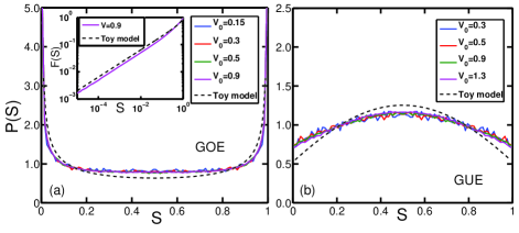
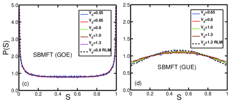
Figure 5: (Color online) The distribution of $S$ (which includes both $|\lambda_{\kappa}-\epsilon_{i}|/|\epsilon_{i+1}-\epsilon_{i}|$ and $|\lambda_{\kappa}-\epsilon_{i+1}|/|\epsilon_{i+1}-\epsilon_{i}|$) for the resonant level model (a) GOE, (b) GUE, and for the SBMFT treatment of the infinite-$U$ Anderson model (c) GOE, (d) GUE. Insert of (a): the cumulative distribution of the $V_{0}=0.9$ GOE data compared to the toy model. The dashed lines in (a) and (b) are the result of the toy model; those in (c) and (d) show the RLM result for $V_{0}=0.9$ and $1.3$, respectively. Parameters: $D=3$, $\epsilon_{0}=0$ for the RLM and $E_{d}=-0.7$ in the SBMFT, 5000 realizations are used, and there are 500 energy levels within the band.

To characterize the relation between the weak and strong coupling levels, we consider the distribution of the normalized level shift defined by

$$S\in\left\{\frac{|\lambda_{\kappa}-\epsilon_{i}|}{|\epsilon_{i+1}-\epsilon_{i}|},\frac{|\lambda_{\kappa}-\epsilon_{i+1}|}{|\epsilon_{i+1}-\epsilon_{i}|}\right\}\;.$$ (81)

The range of $S$ is from $0$ to $1$.

We start by considering the non-interacting RLM, introducing the resonant level right at the chemical potential, $\epsilon_{0}=0$, and then analyzing those levels within the resonant width, $-\Gamma_{0}/2<\lambda_{\kappa}<\Gamma_{0}/2$. Fig. 5 shows the probability distribution $P(S)$ obtained by sampling a large number of realizations. We see that this distribution is independent of the coupling strength (for levels within the resonant width). The corresponding results for the toy model, Eqs. (76) and (V.2), are plotted in Fig. 5 as well. The toy model gives a good overall picture of both the distribution of $S$ and the difference between the orthogonal and unitary cases: the strong coupling levels are concentrated near the original levels in the case of the GOE while they are pushed away from the original levels in the GUE. Quantitatively, however, the weight in the middle of the interval is greater in the full RLM than in the toy model. Comparing the GUE case with the prediction Eq. (V.2) obtained from the second toy model (after performing the proper averaging over $\bar{\lambda}/\bar{\Gamma}$, see Appendix C), we see that this difference can be attributed to the mean effect of the levels other than the closest ones, which tend to push $\lambda_{\kappa}$ into the middle of the interval $[\epsilon_{i},\epsilon_{i+1}]$. Remarkably, as seen in Fig. 5, neglecting the fluctuations of the wave-functions other than $|\phi_{i}(0)|^{2}$ and $|\phi_{i+1}(0)|^{2}$ tends to make this “pressure” toward the center somewhat bigger than it would be if all fluctuations were taken into account.

One intriguing prediction of the toy model is the square root singularity at $S=0$ and $S=1$ in the GOE case. To see whether this is present in the RLM numerical results, we plot the cumulative distribution function on a log-log scale in the inset in Fig. 5; the resulting straight line parallel to the toy model result (though with slightly smaller magnitude) shows that, indeed, the square root singularity is present. As predicted by the toy model, breaking time reversal symmetry causes a dramatic change in $P(S)$.

Results for the full SBMFT treatment of the infinite-$U$ Anderson model are shown in Figs. 5(c) and 5(d) for the GOE and GUE, respectively. Only levels satisfying $\mathcal{E}_{0}-\Gamma(\eta)/2<\lambda_{\kappa}<\mathcal{E}_{0}+\Gamma(\eta)/2$ are included; these are the levels that are within the Kondo resonance. Fig. 5 shows that the perturbed energy levels within the Kondo resonance for the interacting model have the same statistical properties as the ones within the resonance for the non-interacting model.

VI Wave-function correlations

We turn now to the properties of the eigenstates. A key quantity of interest in quantum dot physics is the magnitude of the wave function of a level at a point in the dot that is coupled to an external lead. This quantity is directly related to the conductance through the dot when the chemical potential is close to the energy of the level Kouwenhoven et al. (1997); Kaul et al. (2003). We assume that the probing lead is very weakly coupled, so the relevant quantity is the magnitude of the wave function in the absence of leads. Within our RMT model, all points other than the point $\mathbf{r}=0$, to which the impurity is coupled, are equivalent. The evolution of the magnitude of the quasi-particle wave function probability $|\psi_{i}(\mathbf{r})|^{2}$, at some arbitrary point $\mathbf{r}\neq 0$ as a function of the coupling strength is shown in Fig. 1(c) for GOE and Fig. 2(c) for GUE. Note the large variation in magnitude, often over a narrow window in coupling $V_{0}$, and the fact that the magnitude of each level tends to go to 0 at some value of $V_{0}$ (though not all at the same value).

In order to understand how the coupling to an outside lead at $\mathbf{r}$ is affected by the coupling to the impurity, we study the correlation between the quasi-particle wave-function probability $|\psi_{\kappa(i)}(\mathbf{r})|^{2}$ and the unperturbed wave-function probability $|\phi_{i}(\mathbf{r})|^{2}$ [using the convention of Sec. III.1, $\kappa(i)=i$]. More specifically, we will consider in this section the correlator

$$\mathcal{C}_{i,\kappa(i)}=\frac{\overline{|\phi_{i}(\mathbf{r})|^{2}|\psi_{\kappa(i)}(\mathbf{r})|^{2}}-\overline{|\phi_{i}(\mathbf{r})|^{2}}\cdot\overline{|\psi_{\kappa(i)}(\mathbf{r})|^{2}}}{\sigma(|\phi_{i}(\mathbf{r})|^{2})\sigma(|\psi_{\kappa(i)}(\mathbf{r})|^{2})}\;.$$ (82)

The average $\overline{(\cdot)}$ here is over all realizations, for arbitrary fixed $\mathbf{r}\neq 0$, and $\sigma(\cdot)$ is the square root of the variance of the corresponding quantity.

We expect that, as for the energies, most of the wave-function fluctuation properties can be understood by starting from the RLM Eq. (57) despite the fact that fluctuations of the mean-field parametersmare not included. We start therefore with Fig. 6 which shows $\mathcal{C}_{i,\kappa(i)}$ for the non-interacting RLM as a function of the average distance $\delta\bar{\epsilon}_{i}=(i\Delta-D/2)$ between $\epsilon_{i}$ and $\epsilon_{0}=0$ (which is in the middle of the band). In Fig. 6 (a) and (c), the correlator $\mathcal{C}_{i,\kappa(i)}$ has a dip at the position of the impurity level. The width of the dip increases as the coupling $V_{0}$ increases. Rescaling the energy axis by $\Gamma_{0}$, as done in Fig. 6 (b) and (d), shows that the width of the dip is proportional to the resonance width. One also finds that $\mathcal{C}_{i,\kappa(i)}$ is $\simeq 1$ for the energy levels outside the resonance, which is expected, but that $\mathcal{C}_{i,\kappa(i)}$ is slightly below 1/2 in the center of the resonance.

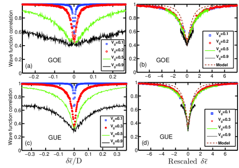
Figure 6: (Color online) Wave function correlator $\mathcal{C}_{i,\kappa(i)}$ for the non-interacting RLM ($\bar{\eta}=1$). (a) GOE and (c) GUE, as a function of the average distance between $\epsilon_{i}$ and $\epsilon_{0}$. (b) GOE and (d) GUE, as a function of rescaled average distance $\epsilon=(i\Delta-D/2)/\Gamma_{0}$. The dashed lines are the result of Eq.(90) in which the wavefunction fluctuations are taken into account but the energy levels are assumed bulk-like. Parameters: $D=3$, impurity energy level $\epsilon_{0}=0$, $5000$ realizations, and $500$ energy levels within the band.

Figure 7: (Color online) Wave function correlation, $\mathcal{C}_{i,\kappa(i)}$, for the SBFMT approach to the infinite-$U$ Anderson model. (a) GOE and (c) GUE, as a function of the average distance from the middle of the band. (b) GOE and (d) GUE, as a function of rescaled average distance $\delta\bar{\epsilon}=[(i\Delta\!-\!D/2)-(\mathcal{E}_{0}(\xi)\!-\!\mu)]/\Gamma(\eta)$. The black lines labeled RLM are results for the non-interacting RLM at $V_{0}=0.5$; The dashed lines are the result of Eq.(90) in which the wavefunction fluctuations are taken into account but the energy levels are assumed bulk-like. Parameters: $D=3$, impurity energy level $E_{d}=-0.7$, $5000$ realizations, and $500$ energy levels within the band.

Turning now to the full self-consistent problem, we plot in Fig. 7 the wave-function correlator $\mathcal{C}_{i,\kappa(i)}$ for the full SBMFT approach to the infinite-$U$ Anderson model. Panels (a) and (c) show that the wave-function correlation has a dip similar to that in the RLM results. The dip is located at $\delta\bar{\epsilon}_{i}=0.0$ for small coupling (i.e. $V_{0}=0.6$), and then moves to larger $\delta\bar{\epsilon}_{i}$ as the coupling $V_{0}$ increases. This is a natural result for the highly asymmetric infinite-$U$ Anderson model: for small coupling, the SBMFT calculation leads to $\mathcal{E}_{0}-\mu=E_{d}-\xi\approx 0$, while for increasing $V_{0}$, $\mathcal{E}_{0}-\mu$ increases to positive values. In fact, the dip corresponds to the effective Kondo resonance. Incorporating the shift of $\mathcal{E}_{0}(\xi)$ and rescaling by $\Gamma(\eta)\sim T_{K}$, we plot the wave function correlation as a function of $\delta\tilde{\epsilon}\equiv[(i\Delta\!-\!D/2)-(\mathcal{E}_{0}(\xi)\!-\!\mu)]/\Gamma(\eta)$ in Fig. 7 (b) and (d). All the curves collapse onto universal curves, one for the GOE and another for the GUE. In addition, the universal curves are the same as the universal curves for the RLM.

As anticipated, the (fixed parameter) resonant level model contains essentially all the physics controlling the behavior of the correlator $\mathcal{C}_{i,\kappa(i)}$. We can therefore try to understand the behavior of this quantity without taking into account the fluctuations of the mean field parameters.

Using again the Green function Eq. (27), we can define the quasi-particle wave-function probability $|\psi_{\kappa}({\bf r})|^{2}$ as the residue at $\lambda_{\kappa}$ of $\langle{\bf r}|\hat{G}|{\bf r}\rangle=\sum_{jj^{\prime}}\psi_{j}({\bf r})G_{jj^{\prime}}\psi_{j^{\prime}}({\bf r})$. From the expression for $G_{jj^{\prime}}$ given in Eq. (II.4), we thus have

$$|\psi_{\kappa}({\bf r})|^{2}=\sum_{jj^{\prime}}\frac{\psi_{j}({\bf r})v^{*}_{j}}{\lambda_{\kappa}-\epsilon_{j}}\cdot u_{\kappa}\cdot\frac{\psi^{*}_{j^{\prime}}({\bf r})v_{j^{\prime}}}{\lambda_{\kappa}-\epsilon_{j^{\prime}}}\;,$$ (83)

where $v_{j}=\eta V_{0}\phi_{j}({\bf 0})$ is the coupling of the state $j$ to the impurity and $u_{\kappa}\equiv|\langle\psi_{\kappa}|f\rangle|^{2}$ is given by Eq. (30). Therefore

$$|\psi_{\kappa}({\bf r})|^{2}\cdot|\phi_{i}({\bf r})|^{2}=\sum_{jj^{\prime}}\Omega^{\kappa}_{jj^{\prime}}\,\psi_{j}({\bf r})\psi^{*}_{j^{\prime}}({\bf r})\psi_{i}({\bf r})\psi^{*}_{i}({\bf r})\;,$$ (84)

where we have defined

$$\Omega^{\kappa}_{jj^{\prime}}\equiv\frac{v^{*}_{j}}{\lambda_{\kappa}-\epsilon_{j}}\cdot u_{\kappa}\cdot\frac{v_{j^{\prime}}}{\lambda_{\kappa}-\epsilon_{j^{\prime}}}\;.$$ (85)

In our random matrix model, there is no correlation between different wave-functions or between wave-functions and energy levels. We thus have

$$\overline{|\phi_{i}(\mathbf{r})|^{2}|\psi_{\kappa}(\mathbf{r})|^{2}}-\overline{|\phi_{i}(\mathbf{r})|^{2}}\cdot\overline{|\psi_{\kappa}(\mathbf{r})|^{2}}=\sum_{jj^{\prime}}\overline{\Omega^{\kappa}_{jj^{\prime}}}\cdot g_{iijj^{\prime}}$$ (86)

where

$$g_{ii^{\prime}jj^{\prime}} \equiv \left[\overline{\psi_{i}({\bf r})\psi^{*}_{i^{\prime}}({\bf r})\psi_{j}({\bf r})\psi^{*}_{j^{\prime}}({\bf r})}\right.$$ (87)

$$-\left.\overline{\psi_{i}({\bf r})\psi^{*}_{i^{\prime}}({\bf r})}\cdot\overline{\psi_{j}({\bf r})\psi^{*}_{j^{\prime}}({\bf r})}\right]\;.$$

Because the wave-functions are independent and Gaussian distributed, $g_{ii^{\prime}jj^{\prime}}=(2/\beta)\delta_{ii^{\prime}}\delta_{jj^{\prime}}\delta_{ij}\overline{|\psi_{i}({\bf r})|^{2}}^{2}$ (remembering the normalization $\overline{|\psi_{i}({\bf r})|^{2}}=1/N$ and $\beta=1$ for GOE while $\beta=2$ for GUE). In the same way, we have $\sigma(|\phi_{i}(\mathbf{r})|^{2})={g_{iiii}}=(2/N\beta)$. Furthermore, using Eq. (83) and the limit $\Gamma\gg\Delta$, we have $\sigma(|\psi_{\kappa}(\mathbf{r})|^{2})\simeq(2/N\beta)$ which then yields

$$\mathcal{C}_{i,\kappa}=\overline{\Omega^{\kappa}_{ii}}=\overline{u_{\kappa}\cdot\frac{|v_{i}|^{2}}{(\lambda_{\kappa}-\epsilon_{i})^{2}}}\;.$$ (88)

[As a side remark, we note that by differentiating Eq. (28) with respect to $\epsilon_{i}$, one can show that $\partial\lambda^{2}_{\kappa}/\partial\epsilon_{i}=\Omega^{\kappa}_{ii}$, and thus $\mathcal{C}_{i,\kappa}=\overline{\partial\lambda_{\kappa}/\partial\epsilon_{i}}$.]

A good approximation to $\mathcal{C}_{i,\kappa(i)}$ can then be obtained from the bulk-value, using Eq. (94) to evaluate (88) in the bulk limit yields

$$\left(\Omega^{\kappa}_{ii}\right)^{\rm bulk}\equiv\Big{[}\displaystyle\delta_{\kappa}^{2}\sum_{i}\frac{1}{(i+\delta_{\kappa})^{2}}\Big{]}^{-1}\;,$$ (89)

where $\delta_{\kappa}=(\lambda_{\kappa(i)}-\epsilon_{i})/\Delta$. Using Eqs. (93), (95), and (96) from Appendix A, we thus have

$$\mathcal{C}_{i,\kappa(i)}\simeq\frac{1}{\left[{\rm cotan}^{-1}\left({\delta\bar{\epsilon}_{i}}/{\Gamma}\right)\right]^{2}\left(1+\left({\delta\bar{\epsilon}_{i}}/{\Gamma}\right)^{2}\right)}\;,$$ (90)

which, as anticipated, depends only on the ratio $({\delta\bar{\epsilon}_{i}}/{\Gamma})$. The curve resulting from this expression is shown in Figs. 6 and 7 and is in good agreement with the numerical data.

Eq. (90) provides a good qualitative and quantitative description of the energy dependence of the correlator $\mathcal{C}_{i,\kappa(i)}$ [although differences between $\left(\Omega^{\kappa}_{ii}\right)^{\rm bulk}$ and $\overline{\Omega^{\kappa}_{ii}}$ are visible]. In a conductance experiment, however, only the levels near the Fermi energy that are within the Kondo resonance contribute to the conductance. In the middle of the resonance, $\mathcal{C}_{i,\kappa(i)}$ is slightly less than one half. At temperatures lower than the mean spacing $\Delta$, for which only one state would contribute to the conductance, there would be some correlation, but only a partial one, between the fluctuations of the conductance in the uncoupled system and the one in the Kondo limit.

VII Discussion and Conclusions

We have obtained results for the correlation between the statistical fluctuations of the properties of the reservoir-dot electrons in two limits: the high-temperature non-interacting gas on the one hand ($T\gg T_{\rm K}^{\rm bulk}$) and, on the other hand, the quasiparticle gas when the Anderson impurity is strongly coupled ($T\ll T_{\rm K}^{\rm bulk}$). The exact treatment of the mesoscopic Kondo problem in the low temperature regime is, however, nontrivial. Since the very low temperature regime ($T\ll T_{\rm K}^{\rm bulk}$) is described by a Nozières-Landau Fermi liquid, we tackled this problem by using the slave boson mean field approximation, through which the infinite-$U$ Anderson model is mapped to an effective resonant level model with renormalized impurity energy level and coupling.

We derived the spectral joint distribution function, Eq. (73), which in principle contains all the information about the correlations between the high and low temperature spectra of the mesoscopic Anderson box. In the spirit of the Wigner surmise, a solvable toy model was introduced to avoid the complications of the joint distribution function. The toy model provides considerable insight into the spectral correlations in the original model.

The numerical infinite-$U$ SBMFT calculation shows the following results. First, the distributions of the mean field parameters are Gaussian. Second, the distribution of the critical coupling $J_{K}^{c}$ does not vanish at zero which shows that there exist some realizations for which the Kondo effect appears at any bare coupling $V_{0}$ and impurity energy level $E_{d}$. Third, for the GOE, the spectral spacing distribution has two sharp peaks at $S=0$ and $S=1$, showing that the two perturbed energy levels (i.e. those for $T\ll T_{\rm K}^{\rm bulk}$) are close to the unperturbed ones ($T\gg T_{\rm K}^{\rm bulk}$). For the GUE, the peak of the spectral correlation function is located at $S=0.5$ corresponding to the center of the two unperturbed energy levels. In addition, the spectral spacing distribution for different coupling strengths $V_{0}$ collapse to universal forms, one for GOE and one for GUE, when we consider only energy levels within the Kondo resonance.

Finally, we studied the influence of the Anderson impurity on the coupling strength between an outside lead and the energy levels of the large dot, as would be probed in a conductance measurement. This is characterized by the intensity of the wave function at an arbitrary point. The correlation function of this intensity corresponding to the unperturbed system and perturbed system shows a dip located at the Kondo resonance, and the width of the dip is proportional to the width of the Kondo resonance. Only the part of the wave function amplitude that corresponds to the perturbed energy levels within the Kondo resonance will be significantly affected due to the coupling to the Kondo impurity.

Appendix A Kondo temperature and values of the mean field parameters in the bulk limit

In this appendix, we provide a brief reminder of the derivation of the Kondo temperature and mean field parameters in the bulk limit. We define this latter by taking $N\to\infty$ and assuming that there are no fluctuations in either the wave-functions nor the unperturbed levels: for all $i$, $x_{i}=1$ and $\epsilon_{i+1}-\epsilon_{i}=\Delta$. We further assume the chemical potential $\mu$ in the middle of the band.

Under these assumptions, the equation defining the Kondo temperature, (39), reads

$$\frac{E_{d}}{\rho_{0}V_{0}^{2}}=\int_{-D/2}^{+D/2}\frac{dy}{y}\tanh{[y/2T_{K}]}=2\ln\left(\frac{a_{K}}{2}\frac{D}{T_{K}}\right)\;,$$ (91)

($a_{K}\simeq 1.1338..$), and thus

$$T_{K}=\frac{a_{K}}{2}D\exp\left(-\frac{|E_{d}|}{2\rho_{0}V_{0}^{2}}\right)\;.$$ (92)

Turning now to the (zero-temperature) mean-field parameters, we shall denote their value in the bulk limit by $\bar{\eta}$ and $\bar{\xi}$, and by $\bar{\Gamma}\equiv\Gamma(\bar{\eta},\bar{\xi})$ and $\mathcal{\bar{E}}_{0}\equiv\mathcal{E}_{0}(\bar{\eta},\bar{\xi})$ the corresponding width and center of the resonance. Let us consider the perturbed eigenlevel $\lambda_{\kappa}\in[\epsilon_{i},\epsilon_{i+1}]$ , and $\delta_{\kappa}\equiv(\lambda_{\kappa}\!-\!\epsilon_{i})/\Delta$. Eq. (28) reads in the bulk limit

$$\frac{\lambda_{\kappa}-\mathcal{\bar{E}}_{0}}{\bar{\Gamma}}=\frac{1}{\pi}\sum_{j}\frac{1}{\delta_{\kappa}-j}\;,$$ (93)

and likewise Eq. (30) for the overlap $u_{\kappa}=|\langle\psi_{\kappa}|f\rangle|^{2}$ is (assuming $\bar{\Gamma}\gg\Delta$)

$$u_{\kappa}=\frac{\pi\Delta}{\bar{\Gamma}}\frac{1}{\sum_{j}{(\delta_{\kappa}-j)^{-2}}}\;.$$ (94)

Using the identities

$$\sum_{j}\frac{1}{\delta_{\kappa}-j} = \pi\,{\rm cotan}(\pi\delta_{\kappa})\;,$$ (95)

$$\sum_{j}\frac{1}{(\delta_{\kappa}-j)^{2}} = \pi^{2}[1+{\rm cotan}^{2}(\pi\delta_{\kappa})]\;,$$ (96)

together with Eq. (93), one obtains

$$\sum_{j}\frac{1}{(\delta_{\kappa}-j)^{2}}=\pi^{2}[1+\frac{(\lambda_{\kappa}-\mathcal{\bar{E}}_{0})^{2}}{\bar{\Gamma}^{2}}]\;.$$ (97)

We therefore can express the bulk analogues $I^{\rm bulk}(\bar{\eta},\bar{\xi})$ and $J^{\rm bulk}(\bar{\eta},\bar{\xi})$ of the sums introduced in the mean-field equations (43)-(44) as

$$I^{\rm bulk}(\bar{\eta},\bar{\xi}) \equiv \int_{-D/2}^{+D/2}dy\frac{{\rm sgn}(y\!-\!\delta\bar{\xi})\,y}{y^{2}+\bar{\Gamma}^{2}}$$ (98)

$$= 2\ln\left(\frac{1}{\sqrt{1+(\delta\bar{\xi}/\bar{\Gamma})^{2}}}\frac{D}{2\bar{\Gamma}}\right)$$

$$J^{\rm bulk}(\bar{\eta},\bar{\xi}) \equiv \frac{1}{\pi\bar{\Gamma}}\int_{-\infty}^{\delta\bar{\xi}}\frac{dy}{1+(y/\bar{\Gamma})^{2}}$$ (99)

$$= \frac{1}{2}+\frac{1}{\pi}\tan^{-1}({\delta\bar{\xi}}/{\bar{\Gamma}})\;.$$

with $\delta\bar{\xi}\equiv(\bar{\xi}\!-\!E_{d})=(\mathcal{\bar{E}}_{0}\!-\!\mu)$.

Eq. (99) inserted into (44) yields

$$\delta\bar{\xi}/\bar{\Gamma}=-\tan(\pi\eta^{2}/2)\;,$$ (100)

which in the Kondo regime $(\eta\ll 1)$ implies $\delta\bar{\xi}/\bar{\Gamma}=O(\eta^{2})$. Inserting Eq. (98) into (43) then gives

$$\bar{\Gamma}=\frac{D}{2}\exp\left(-\frac{|E_{d}|}{2\rho_{0}V_{0}^{2}}\right)$$ (101)

Thus in this regime $T_{\rm K}$ and $\bar{\Gamma}$ differ just by the factor $a_{K}\simeq 1.133$. In the mixed valence regime $T_{K}/\bar{\Gamma}=a_{K}\sqrt{1+\tan^{2}(\pi\eta^{2}/2)}$, which however remains of order one as long as $(1\!-\!\eta^{2})$ does.

As a final comment, we note that Eq. (101) implies $\eta^{2}=(D^{2}/2\pi V_{0}^{2})\exp(-|E_{d}|D/2V_{0}^{2})$, from which we obtain an explicit condition

$$\exp\left(-\frac{1}{\rho_{0}J_{K}}\right)\ll 2\pi\frac{V_{0}^{2}}{D^{2}}$$ (102)

to be in the Kondo regime.

Appendix B Constraint on the sum of the eigenvalues of the resonant level model

In this appendix, we briefly demonstrate Eq. (60) constraining the sum of the eigenvalues of the RLM.

Starting from $\langle\psi_{\kappa}|H_{\rm RLM}|\psi_{\kappa}\rangle=\lambda_{\kappa}\langle\psi_{\kappa}|\psi_{\kappa}\rangle$ we may insert the identity $I=\sum_{i=0}^{N}|i\rangle\langle i|$ on the right hand side (with the notation that $|i=0\rangle\equiv|f\rangle$) and obtain

$$\sum_{i=0}^{N}(\lambda_{\kappa}-\epsilon_{i})\langle\psi_{\kappa}|i\rangle\langle i|\psi_{\kappa}\rangle$$

$$=v\bigg{(}\sum_{i=0}^{N}\phi_{i}(0)\langle f|\psi_{\kappa}\rangle\langle\psi_{\kappa}|i\rangle+{\rm h.c.}\bigg{)}\;.$$

The sum of these equations, $\sum_{\kappa=0}^{N}$, is

$$\sum_{\kappa=0}^{N}\lambda_{\kappa}-\sum_{i=0}^{N}\epsilon_{i} = v\Big{(}\displaystyle\sum_{i,\kappa=0}^{N}\phi_{i}(0)\langle f|\psi_{\kappa}\rangle\langle\psi_{\kappa}|i\rangle+{\rm h.c.}\Big{)}$$ (104)

$$= v\Big{(}\displaystyle\sum_{i=0}^{N}\phi_{i}(0)\delta_{0i}+{\rm h.c.}\Big{)}$$

$$= 0\;;$$

thus, the sum of the two sets of eigenvalues must be equal.

Appendix C Averaging of Eq.(V.2)

Averaging Eq. (V.2) over the variable $\Lambda\equiv\bar{\lambda}/\Gamma$ in some range $[0,\Lambda_{\rm max}]$, we find after a bit of algebra

$$\frac{1}{\Lambda_{\rm max}} \int_{0}^{\Lambda_{\rm max}}P(\sigma)=\frac{4/\pi}{1+2\sigma}\exp\left[-\tilde{f}(\sigma)\right]\times$$

$$\Big{[}\left(1+(1-4\sigma^{2})\tilde{f}^{\prime}(\sigma)+\frac{1-2\sigma}{1+2\sigma}\right)\sinh[\pi(\sigma+\frac{1}{2})\Lambda_{\rm max}]$$

$$-\;\;(\sigma-\frac{1}{2})\tilde{f}(\sigma)\sinh[\pi(\sigma+\frac{1}{2})\Lambda_{\rm max}]$$

$$+\,\pi(\sigma-\frac{1}{2})\Lambda_{\rm max}\cosh[\pi(\sigma+\frac{1}{2})\Lambda_{\rm max}]\Big{]}\;,$$

with $\tilde{f}(\sigma)=f(\sigma,\Lambda\!=\!0)$.

References

- Kondo (1964) J. Kondo, Progress of Theoretical Physics 32, 37 (1964).
- Hewson (1993) A. Hewson, The Kondo Problem to Heavy Fermions (Cambridge University Press, Cambridge, 1993).
- Wilson (1975) K. G. Wilson, Rev. Mod. Phys. 47, 773 (1975).
- Bulla et al. (2008) R. Bulla, T. A. Costi, and T. Pruschke, Rev. Mod. Phys. 80, 395 (2008).
- Andrei (1980) N. Andrei, Phys. Rev. Lett. 45, 379 (1980).
- Wiegmann (1980) P. B. Wiegmann, Physics Letters A 80, 163 (1980).
- Giamarchi (2004) T. Giamarchi, Quantum Physics in One Dimension (Oxford University Press, Oxford, 2004).
- Schotte and Schotte (1969) K. D. Schotte and U. Schotte, Phys. Rev. 182, 479 (1969).
- Schotte (1970) K. D. Schotte, Zeitschrift für Physik A 230, 99 (1970).
- Blume et al. (1970) M. Blume, V. J. Emery, and A. Luther, Phys. Rev. Lett. 25, 450 (1970).
- Anderson (1970) P. W. Anderson, J. Phys. C: Solid State Physics 3, 2436 (1970).
- Fowler and Zawadowzki (1971) M. Fowler and A. Zawadowzki, Solid State Communications 9, 471 (1971).
- Lee et al. (2006) P. A. Lee, N. Nagaosa, and X. Wen, Rev. Mod. Phys. 78, 17 (2006).
- Lacroix and Cyrot (1979) C. Lacroix and M. Cyrot, Phys. Rev. B 20, 1969 (1979).
- Coleman (1983) P. Coleman, Phys. Rev. B 28, 5255 (1983).
- Read et al. (1984) N. Read, D. M. Newns, and S. Doniach, Phys. Rev. B 30, 3841 (1984).
- Nozières (1974) P. Nozières, J. Low Temp. Phys. 17, 31 (1974).
- Ng and Lee (1988) T. K. Ng and P. A. Lee, Phys. Rev. Lett. 61, 1768 (1988).
- Glazman and Raikh (1988) L. Glazman and M. Raikh, Pis’ma Zh. Eksp. Teor. Fiz. 47, 378 (1988), [JETP Lett. 47 (1988) 452].
- Goldhaber-Gordon et al. (1998) D. Goldhaber-Gordon, H. Shtrikman, D. Mahalu, D. Abusch-Magder, U. Meirav, and M. Kastner, Nature 391, 156 (1998).
- Cronenwett et al. (1998) S. M. Cronenwett, T. H. Oosterkamp, and L. P. Kouwenhoven, Science 281, 540 (1998).
- van der Wiel et al. (2000) W. G. van der Wiel, S. D. Franceschi, T. Fujisawa, J. M. Elzerman, S. Tarucha, and L. P. Kouwenhoven, Science 289, 2105 (2000).
- Grobis et al. (2007) M. Grobis, I. G. Rau, R. M. Potok, and D. Goldhaber-Gordon, in Handbook of Magnetism and Advanced Magnetic Materials, Vol. 5, edited by H. Kronmüller and S. Parkin (Wiley, New York, 2007) pp. 2703–2724, arXiv:cond-mat/0611480.
- Chang and Chen (2009) A. M. Chang and J. C. Chen, Rep. Prog. Phys. 72, 096501 (2009).
- Kouwenhoven et al. (1997) L. P. Kouwenhoven, C. M. Marcus, P. L. McEuen, S. Tarucha, R. M. Wetervelt, and N. S. Wingreen, in Mesoscopic Electron Transport, edited by L. L. Sohn, G. Schön, and L. P. Kouwenhoven (Kluwer, Dordrecht, 1997) pp. 105–214.
- Thimm et al. (1999) W. B. Thimm, J. Kroha, and J. von Delft, Phys. Rev. Lett. 82, 2143 (1999).
- Kaul et al. (2005) R. K. Kaul, D. Ullmo, S. Chandrasekharan, and H. U. Baranger, Europhys. Lett. 71, 973 (2005).
- Kettemann (2004) S. Kettemann, in Quantum Information and Decoherence in Nanosystems, edited by D. C. Glattli, M. Sanquer, and J. T. T. Van (The Gioi Publishers, Hannoi, 2004) p. 259, (cond-mat/0409317).
- Kettemann and Mucciolo (2006) S. Kettemann and E. R. Mucciolo, Pis’ma v ZhETF 83, 284 (2006), [JETP Letters 83, 240 (2006); cond-mat:0509251].
- Simon and Affleck (2003) P. Simon and I. Affleck, Phys. Rev. B 68, 115304 (2003).
- Yoo et al. (2005) J. Yoo, S. Chandrasekharan, R. K. Kaul, D. Ullmo, and H. U. Baranger, Phys. Rev. B 71, 201309(R) (2005).
- Kaul et al. (2006) R. K. Kaul, G. Zaránd, S. Chandrasekharan, D. Ullmo, and H. U. Baranger, Phys. Rev. Lett. 96, 176802 (2006).
- Kaul et al. (2009) R. K. Kaul, D. Ullmo, G. Zaránd, S. Chandrasekharan, and H. U. Baranger, Phys. Rev. B 80, 035318 (2009).
- Cornaglia and Balseiro (2002a) P. S. Cornaglia and C. A. Balseiro, Phys. Rev. B 66, 115303 (2002a).
- Cornaglia and Balseiro (2002b) P. S. Cornaglia and C. A. Balseiro, Phys. Rev. B 66, 174404 (2002b).
- Cornaglia and Balseiro (2003) P. S. Cornaglia and C. A. Balseiro, Phys. Rev. Lett. 90, 216801 (2003).
- Kang and Shin (2000) K. Kang and S.-C. Shin, Phys. Rev. Lett. 85, 5619 (2000).
- Affleck and Simon (2001) I. Affleck and P. Simon, Phys. Rev. Lett. 86, 2854 (2001).
- Simon and Affleck (2002) P. Simon and I. Affleck, Phys. Rev. Lett. 89, 206602 (2002).
- Simon et al. (2006) P. Simon, J. Salomez, and D. Feinberg, Phys. Rev. B 73, 205325 (2006).
- Pereira et al. (2008) R. G. Pereira, N. Laflorencie, I. Affleck, and B. I. Halperin, Phys. Rev. B 77, 125327 (2008).
- Zaránd and Udvardi (1996) G. Zaránd and L. Udvardi, Phys. Rev. B 54, 7606 (1996).
- Bedrich et al. (2010) R. Bedrich, S. Burdin, and M. Hentschel, Phys. Rev. B 81, 174406 (2010).
- Kettemann and Mucciolo (2007) S. Kettemann and E. R. Mucciolo, Phys. Rev. B 75, 184407 (2007).
- Zhuravlev et al. (2007) A. Zhuravlev, I. Zharekeshev, E. Gorelov, A. I. Lichtenstein, E. R. Mucciolo, and S. Kettemann, Phys. Rev. Lett. 99, 247202 (2007), (arXiv:0706.3456v1).
- Liu et al. (2012) D. E. Liu, S. Burdin, H. U. Baranger, and D. Ullmo, Europhys. Lett. 97, 17006 (2012).
- Bohigas (1991) O. Bohigas, in Chaos and Quantum Physics, edited by M. J. Giannoni, A. Voros, and J. Jinn-Justin (North-Holland, Amsterdam, 1991) pp. 87–199.
- Mehta (1991) M. L. Mehta, Random Matrices (Second Edition) (Academic Press, London, 1991).
- von Lohneysen et al. (2007) H. von Lohneysen, A. Rosch, M. Vojta, and P. Wolfle, Rev. Mod. Phys. 79, 1015 (2007).
- Fulde et al. (2006) P. Fulde, P. Thalmeier, and G. Zwicknagl, Strongly correlated electrons in Solid State Physics, Vol. 60 (Elsevier, New York, 2006) pp. 1–180.
- Burdin (2009) S. Burdin, in Properties and Applications of Thermoelectric Materials, edited by V. Zlatic and A. Hewson (NATO Science for Peace and Security Series B (9), Springer, Dordrecht, 2009) p. 325, (arXiv:0903.1942).
- Affleck et al. (1988) I. Affleck, Z. Zou, T. Hsu, and P. W. Anderson, Phys. Rev. B 38, 745 (1988).
- Note (1) The chemical potential can be considered as an external tunable parameter, or determined self-consistently if one considers a given electronic occupancy . In this latter case, Eqs. (13)-(14) have to be completed by a third relation: .
- (54) D. Ullmo, D. E. Liu, S. Burdin, and H. U. Baranger, unpublished.
- Fetter and Walecka (1971) A. Fetter and J. Walecka, Quantum Theory of Many-Particle Systems (McGraw-Hill, New York, 1971).
- Nagaoka (1965) Y. Nagaoka, Phys. Rev. 138, A1112 (1965).
- Suhl (1965) H. Suhl, Phys. Rev. 138, A515 (1965).
- Miranda and Dobrosavljevic̀ (2001) E. Miranda and V. Dobrosavljevic̀, Phys. Rev. Lett. 86, 264 (2001).
- Cornaglia et al. (2006) P. S. Cornaglia, D. R. Grempel, and C. A. Balseiro, Phys. Rev. Lett. 96, 117209 (2006).
- Schechter (1959) S. Schechter, Mathematical Tables and Other Aids to Computation 13 (1959).
- Kaul et al. (2003) R. K. Kaul, D. Ullmo, and H. U. Baranger, Phys. Rev. B 68, 161305(R) (2003).