The Realization of the Sharpe-Singleton Scenario
Abstract
The microscopic spectral density of the Wilson Dirac operator for two flavor lattice QCD is analyzed. The computation includes the leading order corrections of the chiral Lagrangian in the microscopic limit. The result is used to demonstrate how the Sharpe-Singleton first order scenario is realized in terms of the eigenvalues of the Wilson Dirac operator. We show that the Sharpe-Singleton scenario only takes place in the theory with dynamical fermions whereas the Aoki phase can be realized in the quenched as well as the unquenched theory. Moreover, we give constraints imposed by -Hermiticity on the additional low energy constants of Wilson chiral perturbation theory.
I Introduction
In the deep chiral limit, with almost massless quarks, lattice QCD with Wilson fermions has a highly nontrivial phase structure. As in continuum QCD, it is the deep chiral limit which reveals the spontaneous breaking of chiral symmetry on the lattice. In addition, the interplay between the continuum and the chiral limit in lattice QCD with Wilson fermions leads to new phase structures known as the Aoki phase Aokiclassic and the Sharpe-Singleton scenario SharpeSingleton . These phases have no direct analogues in the continuum theory, and dominate if the chiral limit is performed prior to the continuum limit. While this at first may seem like a highly undesirable artifact of Wilson fermions it can in fact be turned to our advantage: The Aoki phase is reached through a second order phase transition and at the boundary of this transition the pions are massless. This opens the possibility to study nonperturbative QCD at extremely small pion masses even at a nonzero lattice spacing. On the contrary the Sharpe-Singleton scenario is a first order phase transition in which the pions are massive even in the chiral limit at nonzero lattice spacing.
These phase structures of lattice QCD with Wilson fermions can be described within the framework of Wilson chiral perturbation theory SharpeSingleton ; RS ; BRS ; Aoki-spec ; GSS ; Shindler ; BNSep . This low energy effective theory of lattice QCD with Wilson fermions describes discretization effects by means of additional terms in the chiral Lagrangian (see Golterman ; sharpe-nara for reviews). Each of these new terms come with a new low energy constant. The sign and magnitude of these constants reflect whether lattice QCD with Wilson fermions will enter the Aoki phase or the Sharpe-Singleton scenario. Considerable progress, both analytically DSV ; ADSVprd ; HS1 ; HS2 ; SVlat2011 ; SVtwist and numerically NS ; arXiv:0709.4564 ; 757044 ; arXiv:0911.5061 ; DWW ; DHS ; BBS , has been made recently in the determination of these constants. However, a complete picture has not yet emerged. For example, the observation that quenched lattice simulations consistently observe the Aoki phase Aoki:1992nb ; Aoki:1990ap ; Aoki:1989rw ; Jansen:2005cg , while in unquenched simulations both the Aoki and the Sharpe-Singleton scenario Aoki:1995yf ; Aoki:1997fm ; Ilgenfritz:2003gw ; CERN1 ; CERN2 ; CERN3 ; Aoki:2004iq ; BBS ; Farchioni:2004us ; Farchioni:2004fs ; Farchioni:2005tu ; arXiv:0911.5061 has been observed, remains a puzzle.
The spontaneous breaking of chiral symmetry is tightly connected to the smallest eigenvalues of the Dirac operator BC ; Giusti:2008vb . Moreover, the Aoki phase manifests itself in the smallest eigenvalues of the Wilson Dirac operator Heller ; DSV . Here we show that the behavior of the smallest eigenvalues of the Wilson Dirac operator is also directly related to the Sharpe-Singleton scenario. In particular, we explain that in the Sharpe-Singleton scenario the Wilson Dirac eigenvalues undergo a collective macroscopic jump as the quark mass changes sign. Moreover, we show that this collective jump only occurs in the presence of dynamical fermions. The quenched theory has no analogue of this and hence the Sharpe-Singleton scenario is not possible in the quenched theory. This conclusion is verified by a direct computation of the microscopic quenched and unquenched chiral condensate.
In order to establish these results we explicitly derive the unquenched microscopic spectral density of the Wilson Dirac operator. This calculation makes use of both Wilson random matrix theory as well as Wilson chiral perturbation theory. By means of an underlying Pfaffian structure we uncover a compact factorized form of the exact unquenched microscopic eigenvalue density. This form makes it possible to understand the full dependence of the eigenvalue density on the low energy constants. We analyze this dependence in the mean field limit which can also be directly derived from Wilson chiral perturbation theory.
The mean field limit of the microscopic spectral density corresponds to the leading order result of Wilson chiral perturbation theory in the -regime. This will allow us to close the circle by explaining the original -regime results of Sharpe and Singleton in terms of the behavior of the Wilson Dirac eigenvalues. In particular, we will explain how the nonzero minimal value of the pion mass in the Sharpe-Singleton scenario is connected to the collective jump of the Wilson Dirac eigenvalues.
The approach to the Wilson Dirac spectrum followed in this paper has been applied previously in Refs. sharpe ; DSV ; ADSVprd ; NS ; ADSVNf1 ; SV-Nf2 ; KVZ ; AN ; SVlat2011 ; SVtwist ; K and results from these studies will be used.
The study of the smallest eigenvalues of the Wilson Dirac eigenvalues not only explains the way in which the Aoki phase and the Sharpe-Singleton scenarios are realized, it also gives direct information on the sign and magnitude of the low energy constants of Wilson chiral perturbation theory. We will show that the spectral properties of the Wilson Dirac operator determine the sign of all three additional low energy constants of the leading order chiral Lagrangian of Wilson chiral perturbation theory in the microscopic limit.
The results for the unquenched spectral density of the Wilson Dirac operator presented here also offer a direct way to measure the low energy constants of Wilson chiral perturbation theory by matching the predictions against results from lattice QCD. The first quenched studies of this nature appeared recently DWW ; DHS .
This paper is organized as follows. After a brief presentation of the properties of the Wilson Dirac operator in Section II we recall the basics of Wilson chiral perturbation theory in section III. In section IV we determine constraints on the additional low energy parameters of Wilson chiral perturbation theory in terms of the spectral properties of the Wilson Dirac operator. The unquenched microscopic spectrum of the Wilson Dirac operator is analyzed in section V. Finally, the realization of the Sharpe-Singleton scenario is the topic of section VI. Section VII contains our summary and conclusions. Wilson random matrix theory, the factorization properties of the spectral density and the details of the mean field calculation are discussed in Appendix A, Appendix B and Appendix C, respectively.
II The Wilson Dirac operator
Here we recall a few basic properties of the Wilson Dirac operator. The Wilson term in the lattice discretized covariant derivative
| (1) |
breaks the anti-Hermiticity as well as the axial symmetry of the continuum Dirac operator. However, is -Hermitian
| (2) |
and the product with , is therefore Hermitian.
The eigenvalues, , of consists of complex conjugated pairs as well as exactly real eigenvalues Itoh . Only the real eigenmodes have nonzero chirality and determine the index, , of the Wilson Dirac operator
| (3) |
Here denotes the ’th eigenstate of . The eigenvalues, , of are unpaired when .
In section IV below we will use these properties to constrain the parameters of Wilson chiral perturbation theory.
III Wilson Chiral Perturbation Theory
In the microscopic limit at nonzero lattice spacing where ( is the quark mass, the axial quark mass, an eigenvalue of , and is the lattice spacing)
| (4) |
are kept fixed as , the microscopic partition function of GL extends to DSV
| (5) |
where the action for degenerate quark masses is given by SharpeSingleton ; RS ; BRS
In addition to the chiral condensate, , the action also contains the low energy constants , and as parameters 111Note that we use the convention of DSV ; ADSVprd for the low energy constants , and . In BRS these constants are denoted by , and respectively..
In order to lighten the notation we introduce the rescaled, dimensionless variables
| (7) |
The generating functional for the eigenvalue density of in the complex plane is the graded extension of Eq. (5). Because of the non-Hermiticity of , the graded extension
| (8) |
requires an extra pair of conjugate quarks with masses and , as well as a conjugate pair of bosonic quarks, with masses and Toublan:1999hx . The graded mass term becomes
| (9) |
where Trg denotes the graded trace , with the fermion-fermion block of and its boson-boson block. The eigenvalue density of in the complex plane is
| (10) |
The sign and magnitude of , and determine the phase structure at small mass SharpeSingleton : for the Aoki phase dominates if while for the Sharpe-Singleton scenario takes place. It is therefore of considerable interest to understand if it is possible to determine the signs of the additional low energy constants. In the next section we show how these signs follow from the -Hermiticity of the Wilson Dirac operator.
IV Constraints on , and due to -Hermiticity
In Refs. ADSVprd ; HS1 ; SVtwist it was shown that properties of the partition function and the correlation functions due to -Hermiticity lead to bounds on , and . The bounds that where found are ADSVprd ; HS1 (independent of the value of and HS1 ) and ADSVprd ; SVtwist . In addition it was argued in SVtwist that provided that disconnected diagrams are suppressed. Note that lattice studies arXiv:0709.4564 have found that disconnected diagrams can have a significant contribution.
Here we show that the signs of and can be determined from -Hermiticity if we consider the spectral properties of the Wilson Dirac operator. There are two implicit assumptions that have been well established in the study of Dirac spectra. First, that for a given value of the low-energy constants the chiral Lagrangian can be extended to partially quenched QCD with the same low-energy constants. Second, there is a one-to-one relation between spectral properties in the microscopic domain and the partially quenched chiral Lagrangian.
Let us first recall why -Hermiticity implies that when ADSVprd . As shown by explicit calculations in DSV ; ADSVprd ; ADSVNf1 ; SV-Nf2 the microscopic graded generating functional corresponding to
| (11) |
with gives predictions for the spectrum of the -Hermitian and the Hermitian . This was further confirmed by its equivalence to a -Hermitian Wilson Random Matrix Theory.
On the contrary if , it was explicitly shown in ADSVprd that the graded generating functional corresponding to Eq. (11) is the generating functional for the spectral fluctuations in a lattice theory with iWilson fermions defined as
| (12) |
which is anti-Hermitian rather than -Hermitian. This conclusion was again confirmed by the equivalence to an anti-Hermitian iWilson Random Matrix Theory. Note that and only differ by a factor of in the Wilson term, and that is -Hermitian.
Therefore we understand the effective theory, Eq. (11), for both signs of and that the Hermiticity properties of the Wilson Dirac operator determine this sign. For Wilson fermions we have , whereas for iWilson fermions the constraint is . This is fully consistent with the results from QCD inequalities ADSVprd ; HS1 .
Let us now extend the argument to also include and . We will show that Wilson chiral perturbation theory with , and gives predictions for the spectrum of a -Hermitian . On the contrary Wilson chiral perturbation theory with , and gives predictions for the spectrum of .
The fact that all three signs are reversed when changing between Wilson and iWilson fermions is not accidental. Since the Wilson term and the iWilson term break chiral symmetry in exactly the same way, the respective low energy effective theories, must have the same symmetry breaking terms in the chiral Lagrangian. Moreover, since the explicit symmetry breaking terms at order have their origin in the Wilson term, the two effective fermionic Lagrangians are related by a combined change of sign of , and 222This duality of the Wilson and iWilson fermion lattice theories is due to the fact that the two are related by an axial transformation and an interchange and : The axial transformation and takes . The corresponding transformation on the Goldstone field is ..
In order to see which sign of and corresponds to Wilson fermions let us rewrite the trace squared terms in Wilson chiral perturbation theory as
| (13) | |||||
valid for and and
| (14) | |||||
valid for and .
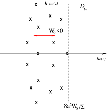
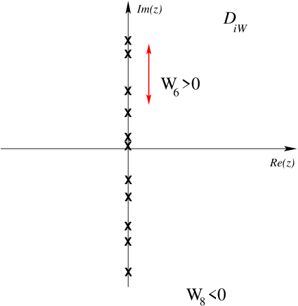
Let us first consider the case . A negative value of corresponds to a Dirac operator that is compatible with the -Hermiticity of the Wilson Dirac operator. The additional fluctuations can be interpreted as collective fluctuations of the eigenvalues, , of parallel to the real -axis. To see this, extend Eq. (13) to the graded generating functional, Eq. (8), and include in the graded mass matrix
| (15) |
(see Eq. (V.1) below for further details). Such fluctuations are allowed for Wilson fermions since the eigenvalues of come in pairs or are strictly real. This is illustrated in the left hand panel of figure 1.
For a positive value of the corresponding Dirac operator is in a different Hermiticity class than the Wilson Dirac operator and will have different spectral properties. Therefore, we necessarily have for the Wilson Dirac operator. For the iWilson-lattice theory on the other hand, we have that and consequently purely imaginary eigenvalues. Moreover, since the eigenvalues are not paired with equal and opposite sign (for ) the spectrum of can fluctuate along the imaginary axis, see the right hand panel of figure 1 for an illustration. The Dirac operator corresponding to is hence in the Hermiticity class of . In perfect agreement with the above conclusion for Wilson fermions and the fact that the two effective theories should have opposite signs for all three ’s.
The story for is analogous: A negative value of corresponds to real fluctuations of the axial quark mass, which are compatible with the Hermiticity properties of the Wilson Dirac operator. These fluctuations can be interpreted as collective fluctuations of the eigenvalues, , of parallel to the real -axis. Such fluctuations are allowed for Wilson fermions since is Hermitian and the symmetry ) is violated when .
For iWilson fermions the product has complex eigenvalues which come in pairs with opposite real part (or are strictly imaginary), hence their fluctuations can only take part in the imaginary direction. This is consistent with in the chiral Lagrangian for iWilson fermions and in perfect agreement with the fact that this sign should be opposite to that of the chiral Lagrangian for Wilson fermions.
Finally, when and have opposite signs the Hermiticity properties of the shifted Dirac operator always differ from the one realized at . The corresponding Dirac operator therefore is neither -Hermitian nor anti-Hermitian. The same is true if all have the same sign.
In conclusion, we explained that the signs of the low energy constants of Wilson chiral perturbation theory follow from the -Hermiticity of the Wilson Dirac operator. We have, , and . Note that both the Aoki phase with and the Sharpe-Singleton scenario with are allowed by -Hermiticity.
In the reminder of this paper we will work with , and . Moreover, since the low energy constant does not affect the competition between the Aoki phase and the Sharpe-Singleton scenario we will set .
In section VI below we show how a collective effect on the eigenvalues of induced by leads to a shift between the Aoki and the Sharpe-Singleton scenario. To establish this result we will first derive the unquenched microscopic eigenvalue density of .
V The unquenched spectrum of
In this section we calculate the microscopic spectral density of the Wilson Dirac operator, , in the presence of two dynamical flavors. We first carry through the calculation with and subsequently introduce the effects of . In order to derive the microscopic spectral density of it is convenient to use Wilson chiral random matrix theory introduced in DSV , which is reviewed in Appendix A for completeness.
We start from the joint eigenvalue probability distribution of the random matrix partition function Eq. (46). To obtain the eigenvalue density in the complex plane we integrate over all but a complex pair of eigenvalues. Using the properties of the Vandermonde determinant we obtain ()
This amazingly compact form can be simplified further. In K it was shown that the four flavor partition function can be expressed in terms of two flavor partition functions. A proof in terms of chiral Lagrangians is given in Appendix B. This leads to the final form for the microscopic spectral density of with two dynamical flavors
where the two flavor partition function is given by SV-Nf2
| (18) | |||||
with
| (21) |
and we have introduced the notation .
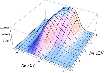
The expression in the first line of Eq. (V) is the quenched eigenvalue density of KVZ . The correction factor in the second line is responsible for the eigenvalue repulsion from the quark mass. A plot of the eigenvalue density of the Wilson Dirac operator in the complex plane for two dynamical flavors is given in figure 2.
Note the strong similarity with the result for the eigenvalue density of the continuum Dirac operator at nonzero chemical potential in phase quenched QCD AOSV . In that case the eigenvalue density follows from the integrable Toda lattice hierarchy Toda . The analytical form of the eigenvalue density of the Wilson Dirac operator, Eq. (V), strongly suggests that a similar integrable structure is present in the microscopic limit of the Wilson lattice QCD partition function.
V.1 Including the effect of
As pointed out in ADSVprd the graded generating function for the eigenvalue density can be extended to include the effect of and by a Gaussian integral as in Eq. (13). Since this works for the graded generating functional it also works for the spectral density itself ADSVprd . In the unquenched case, however, one must be careful with the normalization factor .
Let us start with the case where . Then the density of in the complex plane is obtained from the graded generating function as follows
| (22) | |||||
where the graded generating functional, , was introduced in Eq. (8).
To extend this to we first note that the Gaussian trick, Eq. (13), also works for the graded generating functional. Using this we find
where we will recall the notation: .
In order to understand the effect of on the unquenched spectral density of we will analyze the mean field limit of Eq. (V.1). As is shown in the next section the factor of in the integrand, is essential for the realization of the Sharpe-Singleton scenario.
VI The Sharpe-Singleton Scenario in the spectrum of
Here we show that the Sharpe-Singleton scenario can be understood in terms of a collective effect of the eigenvalues of induced by when the quark mass changes sign. The Sharpe-Singleton scenario is therefore not realized in the quenched theory even if .
Before we give the proof let us first consider an electrostatic analogy which can help set the stage. The quenched chiral condensate
| (24) |
can be thought of as the electric field (in two dimensions) created by positive charges located at the positions of the eigenvalues of and measured at the position (which can be thought of as a test charge). At the point where the quark mass hits the strip of eigenvalues of centered on the imaginary axis, the mass dependence of the chiral condensate (electric field) shows a kink. As the quark mass is lowered further (the test charge passes through the strip of eigenvalues) the condensate (electric field) drops linearly to zero at . The drop is linear because the eigenvalue density is uniform.
For the unquenched chiral condensate we reach an identical conclusion provided that the quark mass (test charge) only has a local effect on the eigenvalues, i.e. it only affects eigenvalues close to the quark mass. This is the case for the Aoki phase when the quark mass is inside the strip of eigenvalues of .
On the contrary, in order to realize the first order Sharpe-Singleton scenario the quark mass must have a collective effect on the eigenvalues of such that the strip of eigenvalues is entirely to the left of the quark mass for small positive values of and then at the strip collectively jumps to the opposite side of the origin such that for small negative values of the quark mass the strip of eigenvalues is to the right of . The collective jump of the eigenvalues at flips the sign of the chiral condensate (electric field) in agreement with the Sharpe-Singleton scenario.
In order to show that the Sharpe-Singleton scenario is indeed realized in terms of the eigenvalues of in the manner described above let us analyze the effect of on the eigenvalues of .
VI.1 The mean field eigenvalue density of
In the mean field limit the density of eigenvalues of at is simply given by a uniform strip of half width centered on the imaginary axis (the deriviation of this result is analogous to the one for nonzero chemical potential, see Toublan:1999hx ; Osborn:2008ab )
| (25) |
This result is identical to the quenched mean field spectral density since the correction factor in the second line of Eq. (V) only has an effect on the microscopic scale (the direct repulsion of the eigenvalues from the quark mass has a microscopic range).
To include the effect of we use the Gaussian trick discussed in Eq. (V.1). The simplest way to proceed is to take the mean field limit before the -integration, we find
Note the essential way in which the two flavor partition function enters both in numerator and the denominator. This is what separates the mean field calculation with dynamical fermions from the quenched analogue.
The mean field result for the two flavor partition function with is given by
| (27) |
The dependence can again be restored by means of introducing an additional Gaussian integral. In the mean field limit this results in
Note that when the term in the second line of this equation is absent. The final result for the mean field two flavor eigenvalue density of is
A derivation of this result which includes the fluctuations around the saddle points is given in Appendix C.
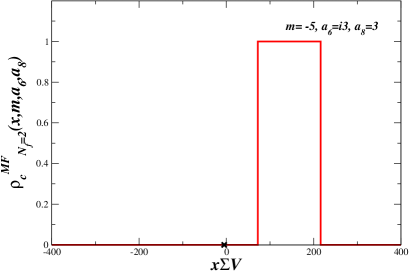
In order to access the Sharpe-Singleton scenario let us consider the case where is small compared to which is taken large and positive.
The terms in the second line of Eq. (VI.1) give rise to a strip of eigenvalues of half width 8 centered at -16 while the term in the third line gives rise to a strip of eigenvalues of half width 8 centered at 16. The relative height of the two strips is . Therefore even though the magnitude of is relatively small it has a dramatic effect: As the sign of changes from positive to negative values the entire strip of eigenvalues jumps from its position around -16 to the new position around 16. For a plot see figure 3. Because of the exponential suppression of one of the strips, the jump of the support of the spectrum occurs on a scale of or and leads to the first order discontinuity of the chiral condensate at as predicted by the Sharpe-Singleton scenario.
In the continuum limit the chiral condensate also jumps from to on a scale of or , but in this case the difference in the potential between the two minima is of as opposed to for the Sharpe-Singleton scenario.
The terms in the mean field two flavor partition function, see Eq. (27), are directly responsible for the jump of the eigenvalue density at in the theory with dynamical quarks. In the corresponding quenched computation we simply have
| (30) |
which leads to a single strip of eigenvalues centered at the imaginary axis independent of the value of
| (31) |
VI.2 The connection to the mean field results of Sharpe and Singleton
From the results of the previous subsection we see that the gap from the quark mass to the edge of the strip of eigenvalues of is given by
| (32) |
In SharpeSingleton it was found that the pion masses for are given by
| (33) |
Hence the gap from the quark mass to the edge of the strip of eigenvalues of can be thought of as the effective quark mass that enters the standard form of the GOR-relation. In particular, note that for the mass never reaches the strip of eigenvalues. Correspondingly, the minimal value of the pion mass is given by
| (34) |
again in perfect agreement with the leading order -regime computation of SharpeSingleton .
VI.3 Direct computation of the quenched and unquenched condensate
From the essential part played by the dynamical fermion determinant in the realization of the Sharpe-Singleton scenario in terms of the eigenvalues of the Wilson Dirac operator we conclude that the Sharpe-Singleton first order scenario only takes place in the theory with dynamical quarks. Here we explicitly compute the quenched and unquenched microscopic chiral condensate and directly verify that the first order jump of the chiral condensate at only takes place in the theory with dynamical quarks.
The unquenched microscopic chiral condensate is obtained from the microscopic partition function by
| (35) |
Specifically, for two mass degenerate flavors we have DSV
with
The quenched condensate was derived in DHS ; ADSVprd
| (38) | |||||
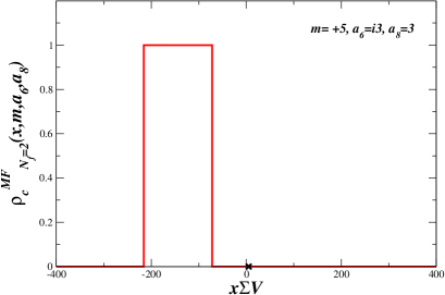
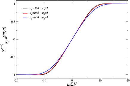
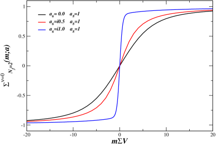
In Refs. DHS ; ADSVprd , its imaginary part was studied since it is directly related to the real eigenvalues of . Here we are after the quenched condensate itself which is given by its real part. Figure 4 compares the behavior of the quenched chiral condensate and the chiral condensate for for three sets of values of and . While the first order jump forms in the thermodynamic limit for the condensate with dynamical quarks when turns negative the kink in the mass dependence of the quenched condensate remains. This directly verifies that the Sharpe-Singleton scenario is absent in quenched theory independent of the value of .
Note that the authors of GSS concluded that both the Aoki phase and the Sharpe-Singleton scenario are possible in the quenched theory. They reached this conclusion because they worked in the large limit in which and vanish, and because the constraint on the sign of was not known at the time.
VII Conclusions
The first order scenario of Sharpe and Singleton for lattice QCD with Wilson fermions has been studied from the perspective of the eigenvalues of the Wilson Dirac operator. The behavior of the Wilson Dirac eigenvalues not only gives constraints on the additional low energy parameters of Wilson chiral perturbation theory (, and ), it also allows us to explain the way in which the first order discontinuity of the chiral condensate is realized. In particular, we have shown that the associated collective jump of the spectrum of the Wilson Dirac operator only occurs in the theory with dynamical quarks. The Sharpe-Singleton scenario is therefore not realized in the quenched theory which enters in the Aoki phase at sufficiently small quark mass. By a direct computation of the quenched microscopic chiral condensate we verified that the second order phase transition occurs in the quenched theory even if . This explains the puzzle why the Aoki phase dominates in the chiral limit of quenched lattice simulations while both the Aoki phase and the Sharpe-Singleton scenario have been observed in lattice QCD with dynamical Wilson fermions.
The above conclusion was made possible by the computation of the exact analytical result for the microscopic spectral density of the Wilson Dirac operator in lattice QCD with two dynamical flavors. The explicit form of the microscopic expression allowed us to compute the mean field eigenvalue density and in turn make a direct connection to the original leading order -regime results of Sharpe and Singleton.
It would be most interesting to test the predictions presented in this paper against dynamical lattice QCD simulations. Since the effects of and on the spectrum of in the unquenched theory are drastically different this offers a direct way to determine the values of these low energy constants. An early lattice study of the Wilson Dirac eigenvalues in dynamical simulations with light quarks appeared in Farchioni:2002vn .
Finally, since the additional low energy constants of Wilson chiral perturbation theory parameterize the discretization errors, it is also most interesting to consider the effects of improvements of the lattice action on the unquenched spectrum of the Wilson Dirac operator Hasenfratz:2007rf .
Acknowledgments: We would like to thank the participants of the ECT∗ workshop ’Chiral dynamics with Wilson fermions’ for useful discussions. This work was supported by the Alexander-von-Humboldt Foundation (MK), U.S. DOE Grant No. DE-FG-88ER40388 (JV) and the Sapere Aude program of The Danish Council for Independent Research (KS).
Appendix A Wilson Random Matrix Theory
In order to derive the microscopic spectral density of it is convenient to use Wilson chiral random matrix theory introduced in DSV .
The partition function of Wilson chiral random matrix theory is defined as
| (39) |
The matrix integrals are over the complex Haar measure.
The random matrix analogue of the Wilson Dirac operator is
| (42) |
where
| (43) |
are and complex matrices, respectively, and is an arbitrary complex matrix. Finally, the weight is
| (44) |
where .
As was shown in Ref. ADSVprd , the Wilson random matrix partition function matches the microscopic partition function of Wilson chiral perturbation theory in the limit with and fixed provided that we identify
| (45) |
An eigenvalue representation of the partition function was derived in KVZ
| (46) |
where are the eigenvalues of and
| (47) |
and
| (48) | |||||
Finally, is the Vandermonde determinant of the eigenvalues.
In section V we use this eigenvalue representation to derive the general form of the unquenched spectral density of .
Appendix B Simplification of the partition function
In this appendix we express the general partition function with even in terms of a Pfaffian of two flavor partition functions. This Pfaffian form was first given in K . Here we give a proof in terms of chiral Lagrangians rather than random matrix theories. In particular, we explicitly express the four flavor partition function entering Eq. (V) in terms of two flavor partition functions.
We start from the general microscopic partition function, Eq. (5), with and make use of the identity
| (49) | |||||
where is an anti-Hermitian matrix and a normalization constant. After a shift of by we obtain
| (50) |
The next step is to decompose with a diagonal matrix and perform the integration over by the Itzykson-Zuber integral. We find
| (51) | |||||
The Vandermonde determinant is defined by
| (52) |
and an explicit expression for the partition function at is given by
We have that
| (54) |
which we will denote by the symbol . We now express as a Pfaffian.
By using recursion relations for Bessel functions, can be rewritten as
| (55) |
where . Writing the determinant as a sum over permutations and splitting the permutations into permutations of odd integers, , even integers, , and the mixed permutations of even and odd integers, , we obtain
| (56) |
The permutation over the even and odd integers can be resummed into a Vandermonde determinant
| (57) |
Next we combine the Vandermonde determinants as
| (58) | |||||
with
| (59) |
The combination can thus be written as
| (60) |
The determinant is a sum over permutations of even and odd integers which together with can be combined into a sum over all permutations
| (61) |
which is equal to the Pfaffian
| (62) |
where we have recovered the Pfaffian structure of K . This leads to K
| (63) |
The alternative proof given here shows that the result is manifestly universal.
Appendix B.1 The four flavor partition function
For the four flavor partition function entering Eq. (V) the Pfaffian structure yields
The latter two terms form a derivative in the limit
With this we have succeeded in expressing the four flavor partition function in terms of the two flavor partition function. This form inserted in Eq. (V) leads to Eq. (V).
Appendix C Mean field including fluctuations
Here we compute the mean field eigenvalue density of including the fluctuations about the saddle points. In Appendix C.1 we derive the mean field limit of the two flavor partition function. A mean field approximation for the four flavor partition function that enters in the spectral density, (V.1), is given in Appendix C.2, and the mean field result for the spectral density is derived in Appendix C.3. We discuss the explicit dependence on the low energy constants and and give the result both for the Aoki phase and the Sharpe-Singleton scenario. As explained in section IV we have and .
Appendix C.1 The two flavor partition function
We consider the two-flavor partition function
From the exponent we recognize that in the mean field limit we always have
| (67) |
For the solution of
| (68) |
is a minimum and does not contribute in the mean field limit (this is the case of the Sharpe-Singleton scenario). Therefore the maxima can only come from
| (69) |
In combination with Eq. (67) this yields the two solutions .
We make the following expansion
| (70) |
The maximum of the two points is at . Thus we obtain the two flavor partition function
for .
For (i.e. in the Aoki phase) the saddlepoint given in Eq. (68), is a maximum. Hence we have to take it into account in the saddlepoint analysis if the right hand side of Eq. (68) is in the interval . Thereby we recognize that there are actually four saddlepoints fulfilling both conditions (67) and (68). The two angles may have the same sign or the opposite one. Those with the same sign are algebraically suppressed by the in the measure.
Let . The expansion about is given by
| (72) |
The simplified integral which we have to solve is
Hence the two flavor partion function is given by
for . Please notice that the second term results from two saddlepoints at and only appears in a certain range of the quark mass. Moreover the result (Appendix C.1) is also valid for since the Heavyside distribution vanishes in this regime.
Appendix C.2 The modified four flavor partition function
We consider the four flavor partition function which for can be written as
The permutation group of four elements is denoted by .
In the mean field limit we have to expand the partition function about the maxima of the exponent. Omitting the permutations we identify two imediate conditions,
| (76) |
This is solved by
| (77) |
Other choices are supressed by the Vandermonde determinant. Hence we have to maximize the function
| (78) | |||||
We consider the case (the Sharpe-Singleton scenario). Therefore the extremum for is a minimum and not a maximum. The situation would be completely different for , see discussion after Eq. (87).
The maximum of for all is given by
| (79) |
This result takes its maximum at yielding
| (80) |
In the integral (Appendix C.2) this maximum should be inside the interval
| (81) |
The condition for the second integral is then
| (82) |
We make the following expansion
| (83) | |||||
This expansion is substituted into Eq. (Appendix C.2) and we omit the sum since each term gives the same contribution and the degeneracy of the maximum,
This integral decouples into two two-fold integrals. We need the following integral for large ,
| (85) |
where is the error function and use the identity
| (86) | |||||
Then the final result for the partition function is given by
| (87) | |||||
for (in the Sharpe Singleton scenario).
In the Aoki phase, , the extremum for is a maximum, cf. Eq. (78). However it will only contribute if
| (88) |
and
| (89) |
Then the saddlepoint changes to
| (90) | |||||
Hence the expansion about the saddle points is given by
| (91) | |||||
The degeneracy of this maximum is four which results in the integral
| (92) | |||||
Combining this with the result (87) for we find
| (93) | |||||
This formula applies to both scenarios since the Heavyside distribution puts the second term to zero in the Sharpe-Singleton scenario.
Appendix C.3 The unquenched level density
Combining the mean field limit of the numerator and denominator of Eq. (V.1) given by Eq. (Appendix C.1) and Eq. (93), respectively, we obtain
independent of the value of . The first term will drop out if we are in the Aoki phase whereas the second term vanishes in the Sharpe-Singleton scenario. However the reason for this mechanism is quite different in the two cases. In the Aoki phase the first term is exponentially supressed in comparison to the second one which results from the extremum (90). In the Sharpe-Singleton scenario the saddlepoint is a minimum and enters a priori not in the saddlepoint analysis. Hence we have to look at the boundaries of the four dimensional box spanned by the four cosinus, see the discussion in Appendix C.2.
This mechanism explains why we find a second order transition in the Aoki phase and a first order transition in the Sharpe-Singleton scenario. The extremum (90) can cross the four dimensional box with varying quark mass and eigenvalue . Hence we have a continuous process from one boundary to the other in the Aoki scenario. When this extremum is excluded as in the Sharpe-Singleton scenario, the maximum has to jump from one boundary to the other. This manifests itself in the sign of the mass in the Heavyside distribution of the first term and the mass itself in the other one.
References
- (1) S. Aoki, Phys. Rev. D 30 (1984) 2653.
- (2) S. R. Sharpe and R. L. Singleton, Phys. Rev. D 58, 074501 (1998) [hep-lat/9804028].
- (3) G. Rupak and N. Shoresh, Phys. Rev. 66, 054503 (2002), [arXiv:hep-lat/0201019].
- (4) O. Bär, G. Rupak and N. Shoresh, Phys. Rev. D 70, 034508 (2004), [arXiv:hep-lat/0306021].
- (5) S. Aoki, Phys. Rev. D 68, 054508 (2003) [arXiv:hep-lat/0306027].
- (6) M. Golterman, S. R. Sharpe and R. L. Singleton, Phys. Rev. D 71, 094503 (2005) [arXiv:hep-lat/0501015].
- (7) A. Shindler, Phys. Lett. B 672, 82 (2009) [arXiv:0812.2251 [hep-lat]].
- (8) O. Bär, S. Necco, and S. Schaefer, J. High Energy Phys. 03 (2009) 006.
- (9) M. Golterman, arXiv:0912.4042.
- (10) S. R. Sharpe, arXiv:hep-lat/0607016.
- (11) P. H. Damgaard, K. Splittorff and J. J. M. Verbaarschot, Phys. Rev. Lett. 105, 162002 (2010). [arXiv:1001.2937 [hep-th]].
- (12) G. Akemann, P. H. Damgaard, K. Splittorff, J. J. M. Verbaarschot, Phys. Rev. D 83, 085014 (2011) [arXiv:1012.0752 [hep-lat]].
- (13) M. T. Hansen and S. R. Sharpe, Phys. Rev. D 85, 014503 (2012) [arXiv:1111.2404 [hep-lat]].
- (14) M. T. Hansen and S. R. Sharpe, arXiv:1112.3998 [hep-lat].
- (15) K. Splittorff and J. J. M. Verbaarschot, arXiv:1112.0377 [hep-lat].
- (16) K. Splittorff and J. J. M. Verbaarschot, arXiv:1201.1361 [hep-lat].
- (17) S. Necco and A. Shindler, JHEP 1104, 031 (2011) [arXiv:1101.1778 [hep-lat]].
- (18) C. Michael et al. [ETM Collaboration], PoSLAT 2007, 122 (2007) [arXiv:0709.4564 [hep-lat]].
- (19) S. Aoki and O. Bär, Eur. Phys. J. A 31, 781 (2007).
- (20) R. Baron et al. [ETM Collaboration], JHEP 1008, 097 (2010) [arXiv:0911.5061 [hep-lat]].
- (21) A. Deuzeman, U. Wenger and J. Wuilloud, JHEP 1112, 109 (2011) [arXiv:1110.4002 [hep-lat]].
- (22) P. H. Damgaard, U. M. Heller and K. Splittorff, Phys. Rev. D 85, 014505 (2012) [arXiv:1110.2851 [hep-lat]].
- (23) F. Bernardoni, J. Bulava and R. Sommer, arXiv:1111.4351 [hep-lat].
- (24) S. Aoki and A. Gocksch, Phys. Rev. D 45, 3845 (1992).
- (25) S. Aoki and A. Gocksch, Phys. Lett. B 243, 409 (1990).
- (26) S. Aoki and A. Gocksch, Phys. Lett. B 231 (1989) 449.
- (27) K. Jansen et al. [XLF Collaboration], Phys. Lett. B 624, 334 (2005) [arXiv:hep-lat/0507032].
- (28) S. Aoki, A. Ukawa and T. Umemura, Phys. Rev. Lett. 76, 873 (1996) [arXiv:hep-lat/9508008].
- (29) S. Aoki, Nucl. Phys. Proc. Suppl. 60B, 206 (1998) [hep-lat/9707020].
- (30) E. -M. Ilgenfritz, W. Kerler, M. Muller-Preussker, A. Sternbeck and H. Stuben, Phys. Rev. D 69, 074511 (2004) [hep-lat/0309057].
- (31) L. Del Debbio, L. Giusti, M. Luscher, R. Petronzio and N. Tantalo, JHEP 0702, 082 (2007) [hep-lat/0701009].
- (32) L. Del Debbio, L. Giusti, M. Luscher, R. Petronzio and N. Tantalo, JHEP 0702, 056 (2007) [hep-lat/0610059].
- (33) L. Del Debbio, L. Giusti, M. Luscher, R. Petronzio and N. Tantalo, JHEP 0602, 011 (2006) [hep-lat/0512021].
- (34) S. Aoki et al. [JLQCD Collaboration], Phys. Rev. D 72, 054510 (2005) [hep-lat/0409016].
- (35) F. Farchioni, R. Frezzotti, K. Jansen, I. Montvay, G. C. Rossi, E. Scholz, A. Shindler and N. Ukita et al., Eur. Phys. J. C 39, 421 (2005) [hep-lat/0406039].
- (36) F. Farchioni, K. Jansen, I. Montvay, E. Scholz, L. Scorzato, A. Shindler, N. Ukita and C. Urbach et al., Eur. Phys. J. C 42, 73 (2005) [hep-lat/0410031].
- (37) F. Farchioni, K. Jansen, I. Montvay, E. E. Scholz, L. Scorzato, A. Shindler, N. Ukita and C. Urbach et al., Phys. Lett. B 624, 324 (2005) [hep-lat/0506025].
- (38) T. Banks, A. Casher, Nucl. Phys. B169, 103 (1980).
- (39) L. Giusti and M. Luscher, JHEP 0903, 013 (2009) [arXiv:0812.3638 [hep-lat]].
- (40) K. M. Bitar, U. M. Heller and R. Narayanan, Phys. Lett. B 418, 167 (1998). [arXiv:hep-th/9710052].
- (41) S. R. Sharpe, Phys. Rev. D 74, 014512 (2006) [arXiv:hep-lat/0606002].
- (42) G. Akemann, P. H. Damgaard, K. Splittorff, J. J. M. Verbaarschot, PoS LATTICE2010, 079 (2010). [arXiv:1011.5121 [hep-lat]].
- (43) K. Splittorff and J. J. M. Verbaarschot, Phys. Rev. D 84, 065031 (2011) [arXiv:1105.6229 [hep-lat]].
- (44) M. Kieburg, J. J. M. Verbaarschot and S. Zafeiropoulos, Phys. Rev. Lett. 108, 022001 (2012) [arXiv:1109.0656 [hep-lat]]; PoS LATTICE 2011, 312 (2011) [arXiv:1110.2690 [hep-lat]].
- (45) G. Akemann and T. Nagao, JHEP 1110, 060 (2011) [arXiv:1108.3035 [math-ph]].
- (46) M. Kieburg, J. Phys. A A 45, 095205 (2012) [arXiv:1109.5109 [math-ph]].
- (47) S. Itoh, Y. Iwasaki and T. Yoshie, Phys. Rev. D 36, 527 (1987).
- (48) J. Gasser and H. Leutwyler, Phys. Lett. B 188, 477 (1987).
- (49) D. Toublan and J. J. M. Verbaarschot, Int. J. Mod. Phys. B 15, 1404 (2001) [hep-th/0001110].
- (50) G. Akemann, J. C. Osborn, K. Splittorff, J. J. M. Verbaarschot, Nucl. Phys. B712, 287-324 (2005). [hep-th/0411030].
- (51) E. Kanzieper, Phys. Rev. Lett. 89, 250201 (2002). [cond-mat/0207745]. K. Splittorff, J. J. M. Verbaarschot, Phys. Rev. Lett. 90, 041601 (2003). [cond-mat/0209594]; Nucl. Phys. B683, 467-507 (2004). [hep-th/0310271]. Nucl. Phys. B695, 84-102 (2004). [hep-th/0402177]. T. Andersson, P. H. Damgaard, K. Splittorff, Nucl. Phys. B707, 509-528 (2005). [hep-th/0410163].
- (52) J. C. Osborn, K. Splittorff and J. J. M. Verbaarschot, Phys. Rev. D 78, 105006 (2008) [arXiv:0807.4584 [hep-lat]].
- (53) F. Farchioni, C. Gebert, I. Montvay and L. Scorzato, Eur. Phys. J. C 26, 237 (2002) [hep-lat/0206008].
- (54) A. Hasenfratz, R. Hoffmann and S. Schaefer, JHEP 0705, 029 (2007) [hep-lat/0702028].