Modelling high redshift Lyman-alpha Emitters

Abstract

We present a new model for high redshift Lyman-Alpha Emitters (LAEs) in the cosmological context which takes into account the resonant scattering of Ly$\alpha$ photons through expanding gas. The GALICS semi-analytic model provides us with the physical properties of a large sample of high redshift galaxies. We implement, in post processing, a gas outflow model for each galaxy based on simple scaling arguments. The coupling with a library of numerical experiments of Ly$\alpha$ transfer through expanding (or static) dusty shells of gas allows us to derive the Ly$\alpha$ escape fraction and profile of each galaxy. Results obtained with this new approach are compared with simpler models often used in the literature.

The predicted distribution of Ly$\alpha$ photons escape fraction shows that galaxies with a low star formation rate have a $f_{\rm esc}$ of the order of unity, suggesting that, for those objects, Ly$\alpha$ may be used to trace the star formation rate assuming a given conversion law. In galaxies forming stars intensely, the escape fraction spans the whole range from 0 to 1. The model is able to get a good match to the UV and Ly$\alpha$ luminosity function data at $3<z<5$. We find that we are in good agreement with both the bright Ly$\alpha$ data and the faint LAE population observed by Rauch et al. (2008) at z $=3$ whereas a simpler constant Ly$\alpha$ escape fraction model fails to do so. Most of the Ly$\alpha$ profiles of our LAEs are redshifted by the diffusion in the expanding gas which suppresses IGM absorption and scattering. The bulk of the observed Ly$\alpha$ equivalent width distribution is recovered by our model, but we fail to obtain the very large values sometimes detected. Our predictions for stellar masses and UV LFs of LAEs show a satisfactory agreement with observational estimates. The UV-brightest galaxies are found to show only low Ly$\alpha$ equivalent widths in our model, as it is reported by many observations of high redshift LAEs. We interpret this effect as the joint consequence of old stellar populations hosted by UV-bright galaxies, and high Hi column densities that we predict for these objects, which quench preferentially resonant Ly$\alpha$ photons via dust extinction.

1 Introduction

Article	Model	Ly$\alpha$ model	Ly$\alpha$ LF	UV LFs of LAEs	UV LFs	IGM	$\sigma_{8}$
Le Delliou et al. (2006)	SAM (GALFORM)	$f_{\rm esc}=$ const.	yes	no	no	no	0.93
Mao et al. (2007)	ST	$f_{\rm esc}={\rm f}_{\rm IGM}\times e^{\rm-{\rm A}_{\lambda}/1.08}$	yes	no	yes	yes	0.80
Kobayashi et al. (2007, 2010)	SAM (Mitaka)	$f_{\rm esc}=$ const./screen/slab	yes	yes	yes	yes	0.90
Nagamine et al. (2010)	GADGET2	$f_{\rm esc}=$ const./Duty cycle	yes	yes	yes	yes	0.90
Tilvi et al. (2009)	GADGET2	$f_{\rm esc}=1$/Duty cycle	yes	no	no	no	0.82
Samui et al. (2009)	PS-ST	$f_{\rm esc}=$ const./Duty cycle	yes	yes	yes	no	0.80
Zheng et al. (2010)	PMM N body	RT in IGM (no dust)	yes	yes	yes	yes	0.82
Dayal et al. (2008)	GADGET2	$f_{\rm esc}=$ exp(-$\tau_{\rm IGM}$) $\times$ const.	yes	yes	no	yes	0.82
this paper	SAM (GALICS)	$f_{\rm esc}=$ RT	yes	yes	yes	yes	0.76

Table 1: Non-exhaustive summary of existing Ly$\alpha$ cosmological models in the litterature. SAM: Semi-analytic model. PS: Press-Schechter formalism. ST: Sheth-Tormen formalism. PMM: Particle Multi Mesh. RT: Radiation transfer

High-redshift star-forming galaxies are expected to produce strong Ly$\alpha$ emission lines (Partridge & Peebles, 1967; Charlot & Fall, 1993; Valls-Gabaud, 1993). Massive, hot stars are intense sources of hydrogen-ionizing UV photons which turn part of the ISM gas into Hii regions. Ly$\alpha$ photons are produced by recombination of this gas. Altough high-redshift Ly$\alpha$ emitting galaxies have long been sought without success, the number of detections has grown quickly during the last decade, thanks to narrow-band searches (Hu et al., 1998; Kudritzki et al., 2000; Shimasaku et al., 2006; Ouchi et al., 2008; Ouchi et al., 2010; Hu et al., 2010), deep spectroscopic follow-ups of UV-selected galaxies (Shapley et al., 2003; Tapken et al., 2007), and deep spectroscopic blind searches (van Breukelen et al., 2005; Rauch et al., 2008).

Although observed samples of high redshift Lyman-alpha Emitters (hereafter LAEs) have become large enough to derive statistical constraints (e.g. Ly$\alpha$ and UV luminosity functions, hereafter LF), uncertainties remain as a result of measurement errors and differences in survey detection thresholds. The physics involved in LAEs, and especially their Ly$\alpha$ escape fractions, are still poorly understood. Indeed, the travel of Ly$\alpha$ photons from their emission regions through the galaxy and the intergalactic medium (IGM) is complicated. The resonant nature of the Ly$\alpha$ line increases dramatically the traveling path of the photons in the optically-thick interstellar gas, enhancing dust absorption even in metal-poor galaxies. Spectroscopic studies of Ly$\alpha$ emitting galaxies (Kunth et al., 1998; Pettini et al., 2001; Dawson et al., 2002; Shapley et al., 2003; Tapken et al., 2004; Tapken et al., 2006; Tapken et al., 2007) have shown that the line profile is complex, and can have many shapes (P-Cygni, redward asymmetry, double bump). The measure of the interstellar absorption lines with respect to Ly$\alpha$ by Shapley et al. (2003) suggests that gas outflows (probably triggered by supernova feedback) of neutral hydrogen take place in those galaxies. Recent spectroscopic measurements led by McLinden et al. (2011) in two z $\sim 3$ LAEs support this idea. An expanding shell of gas surrounding the galaxy is often proposed as an explanation of this feature and the general shape of the Ly$\alpha$ line (Tenorio-Tagle et al., 1999; Mas-Hesse et al., 2003; Verhamme et al., 2006; Dijkstra & Loeb, 2008).

In the past years, there has been an intense investigation on the properties of LAEs in the context of hierarchical galaxy formation, through semi-analytic or ”hybrid” models, or numerical simulations (e.g. Le Delliou et al., 2005; Le Delliou et al., 2006; Kobayashi et al., 2007; Nagamine et al., 2010; Samui et al., 2009). Although the implementation of galaxy formation processes include state-of-the-art prescriptions, the modelling of the complicated mechanisms of Ly$\alpha$ photons transfer in galaxies, and their escape from the galaxies, is usually very sketchy. The authors frequently assume a constant Ly$\alpha$ escape fraction model, and try to reproduce data (i.e Ly$\alpha$ luminosity functions) by adjusting the escape fraction as a free parameter ($f_{\rm esc}=0.02-0.60$ at $3<z<6$ according to models). This approach appears to work in a satisfactory way, as far as it is possible to get a fit of the bright end of the LAE Ly$\alpha$ luminosity function. However, the deduced value of the free parameter $f_{\rm esc}$ is not ”explained”, and these models fail to reproduce the faint LAE population reported by Rauch et al. (2008) at z $\sim 3$, down to a flux of $\sim 10^{-18}\mbox{erg.s}^{-1}.\mbox{cm}^{-2}$.

A duty cycle scenario (in which only a fraction of the galaxies are turned on as LAEs at a given time, or are able to be detected because of selection criteria) has also been invoked to reproduce the observed Ly$\alpha$ LF. Nagamine et al. (2010) report that a stochastic scenario is favoured compared to a constant Ly$\alpha$ escape fraction model as a result of the comparison with observational data. For the duty cycle model, they require a fraction of star forming galaxies observable as LAEs at a given time equal to $0.07$ ($0.20$) at z $=3$ ($6$). Samui et al. (2009) fit their free parameters which contain the Ly$\alpha$ escape fraction and the number of galaxies turned on as LAEs, on the observed Ly$\alpha$ LFs and UV LFs of LAEs. Their duty cycle parameter has to vary with redshift in order to agree with the data.

Tilvi et al. (2009) relate the Ly$\alpha$ luminosity to the halo mass accretion rate, and are able to reproduce the observed Ly$\alpha$ LF by fitting a single parameter, namely the product of the star-formation efficiency and the Ly$\alpha$ timescale. However, they assume that all Ly$\alpha$ photons are able to escape their model galaxies ($f_{\rm esc}=1$), which is not consistent with observations of LAEs and Lyman Break Galaxies (hereafter LBGs) (e.g. Hayes et al., 2010).

More physical models, taking into account the properties of the galaxies (assuming slab and screen-type dust attenuation), have been investigated by Kobayashi et al. (2007, 2010) and Mao et al. (2007). Kobayashi et al. (2007, 2010) need two free parameters to reproduce the Ly$\alpha$ LF data over the redshift range $3<z<6$. Mao et al. (2007) reproduce the Ly$\alpha$ LFs data at z $=4.9,5.7$ and $6.4$, but they need to vary the IGM transmission.

In parallel to these empirical approaches, several Ly$\alpha$ radiation transfer codes have been developed (Zheng & Miralda-Escudé, 2002; Verhamme et al., 2006; Dijkstra et al., 2006; Hansen & Oh, 2006; Laursen & Sommer-Larsen, 2007) including different physics such as dust, gas kinematics, geometry, deuterium, etc. Zheng et al. (2010) perform Ly$\alpha$ radiative transfer through the circumgalactic medium in a cosmological box, but they do not incorporate dust into their model and do not resolve galaxies. Laursen et al. (2009) focus on a few high-resolution galaxies, but the CPU cost of such experiments does not allow one to process large samples of objects. Indeed, carrying out Ly$\alpha$ line transfer in large simulated volumes, and with a resolution high enough to describe the ISM structure and kinematics, is out of CPU reach today. Hence, the need for simplified semi-analytic models remains. A non-exhaustive summary of the LAE models in the literature is given in Table 1.

The purpose of this paper is to make one step further towards a more realistic semi-analytic approach. To this aim, we present a new model for Ly$\alpha$ emission from high redshift galaxies, which relies on two main ingredients. First, we use GALICS (for Galaxies in Cosmological Simulations), a hybrid model of hierarchical galaxy formation in which galaxy formation and evolution are described as the post-processing of outputs of numerical simulations of a large cosmological volume of dark matter (Hatton et al. (2003)). Second, we use a large library of radiation transfer models (Schaerer et al., 2011) computed with an updated version of MCLya (Verhamme et al., 2006), which describes the Ly$\alpha$ transfer through spherical expanding or static shells of neutral gas and dust. We implement a simple shell model in post-processing of GALICS, based on scaling arguments, to infer the shell parameters of the MCLya library for each model galaxy.

The advantage of this model with respect to constant Ly$\alpha$ escape fraction models is that it computes the Ly$\alpha$ escape fraction of each model galaxy according to its physical properties. In addition, it improves on screen or slab models by including the resonant radiative transfer of the Ly$\alpha$ line, and by assuming a geometry and kinematics suggested by the observations. With this new tool, we are able to compare our results with existing statistical data such as Ly$\alpha$ and UV LFs, Ly$\alpha$ equivalent width distributions, stellar masses and the Ando effect (see Ando et al., 2006; Kobayashi et al., 2010).

The outline of the article is as follows. We describe the GALICS galaxy formation model in Sec. 2, and the Ly$\alpha$ and shell models in Sec. 3. In Sec. 4, we present the distributions of Ly$\alpha$ escape fractions we predict, and the Ly$\alpha$ LFs they yield. We discuss how these LFs are impacted by (i) equivalent width selections and (ii) IGM transmission. In Sec. 5, we show that our model matches most statistical constraints (Ly$\alpha$ equivalent width distributions, UV LFs of LAEs, stellar masses and the Ando effect), and we use it to discuss their origin. Finally, Sec. 6 summarizes the results and gives a brief discussion.

2 The GALICS hybrid model

In the present paper, we use an updated version of the GALICS model (Hatton et al., 2003; Blaizot et al., 2004). We briefly describe the relevant details below.

2.1 Dark matter simulation

We use a dark matter cosmological simulation run by the Horizon project using the public version of Gadget (Springel, 2005). This simulation uses $1024^{3}$ particles of mass $m_{\rm p}\sim 8.5\times 10^{7}$M_⊙ to describe the formation and evolution of dark matter (DM) structures in a comoving volume of 100${\rm h}^{-1}$Mpc on a side. It assumes a cosmology and initial conditions which are consistent with WMAP third year results (Spergel et al., 2007), namely: $h=0.73$, $\Lambda=0.76$, $\Omega_{\rm m}=0.24$, $\Omega_{\rm b}=0.04$, and $\sigma_{8}=0.76$.

About 100 snapshots were saved to disk, regularly spaced in expansion factor by $\delta{\rm a}=0.01$. We processed each of these snapshots to identify DM haloes with a friends-of-friends (FOF) algorithm, using a linking length ${\rm b}=0.20$ and keeping only groups with more than 20 particles, i.e. more massive than $1.7\times 10^{9}$M_⊙. This mass resolution is sufficient for our present study, which adresses galaxy formation after reionization (z $<5$), when we expect the intergalactic medium’s temperature to prevent gas from collapsing within dark matter haloes of lower masses (e.g. Okamoto et al., 2008). Finally, we follow Tweed et al. (2009) to construct merger trees from our halo catalogs at all timesteps.

2.2 Baryonic prescriptions

The version of GALICS we use here is an update from Hatton et al. (2003) and Cattaneo et al. (2008), with 3 major differences which are relevant for the present study: (i) the way galaxies get their gas, (ii) the way galaxies form stars, and (iii) the way we compute extinction of UV light by dust.

First, the new paradigm that has emerged in recent years about gas supply into high redshift galaxies (e.g. Dekel & Birnboim, 2006) has led us to replace the classical gas cooling mechanism by filamentary accretion of cold gas. In practice, for the redshift range which we explore here ($3<z<5$), this means that galaxies accrete gas from the IGM at a rate directly proportional to the halo growth, with a delay set by the free-fall time instead of the cooling time.

Second, we use a Kennicutt-type law to model star formation. The low value of $\sigma_{8}$ from WMAP third year results has led us to enhance star formation significantly compared to the local law of Kennicutt (1998), in order to fit high-redshift observations. In practice, we compute the star formation rate as

$$\frac{{\rm SFR}}{M_{\odot}.{\rm yr}^{-1}}={{{\epsilon}}}\times 0.0328\left(\frac{M_{\rm cold,comp}}{10^{11}M_{\odot}}\right)^{1.4}\left(\frac{{R_{\rm comp}}}{1{\rm Mpc}}\right)^{-0.8},$$ (1)

and we assume a Kennicutt IMF (Kennicutt, 1983). $M_{\rm cold,comp}$ and $R_{comp}$ are respectively the mass of cold (i.e neutral) gas in the ISM and the radius of each galaxy component: disc, bulge and burst (see Hatton et al., 2003, for details). ${{{\epsilon}}}$ is the star formation efficiency parameter.

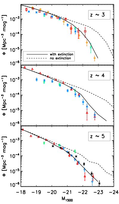
Figure 1: Absolute rest-frame UV LFs (at $1500$ Å) at z $\sim 3,4$ and $5$. In each plot, the solid line refers to the UV LF after extinction while the dashed line represents the non extinguished LF. Data points are from Reddy et al. (2008) (orange diamonds), Arnouts et al. (2005) (red squares), Sawicki & Thompson (2006) (blue asterisks), Gabasch et al. (2004) (green crosses), Bouwens et al. (2007) (red triangles), Iwata et al. (2007) (black asterisks) and McLure et al. (2009) (blue diamonds).

Third, we now compute extinction by dust using a simple screen model, which is consistent with our expanding shell scenario (see Sec. 3), and we introduce a redshift dependency in the dust-to-gas ratio. In practice, we follow Hatton et al. (2003) and write the dust optical depth as

$$\tau_{\rm dust}(\lambda)=\left(\frac{A_{\lambda}}{A_{V}}\right)_{Z_{\odot}}\left(\frac{Z}{Z_{\odot}}\right)^{1.35}\left(\frac{N_{\rm H}}{2.1\times 10^{21}}\right)f(z),$$ (2)

where $(A_{\lambda}/A_{V})_{Z_{\odot}}$ is the extinction curve for solar metallicity taken from Mathis et al. (1983), $Z$ is the metallicity of the absorbing gas (equal to that of the ISM), and $N_{\rm H}$ is the Hi column density. We compute this latter quantity with Eq. 10, written for the expanding shell. It is worth noting, however, that because of our choice of parameters for the shell, Eq. 10 is very similar to that used in Hatton et al. (2003, eq. 6.3). The last term in Eq. 2 introduces a scaling of the dust-to-gas ratio with redshift as $f(z)=(1+z)^{-1/2}$. This scaling is in broad agreement with obervational results of e.g. Reddy et al. (2006), and has already been used in models, e.g. by Kitzbichler & White (2007). Finally, we compute the spectral energy distributions (SEDs) of our model galaxies with the STARDUST library (Devriendt et al., 1999), as in Hatton et al. (2003), and extinguish them using a screen model:

$$L_{\rm obs}(\lambda)=e^{\rm-\tau_{\rm dust}(\lambda)}L_{\rm intrinsic}(\lambda).$$ (3)

Such a model allows us to be consistent both with the physical scenario we implement and with the absorption in the continuum found in the MCLya library (see Sec. 3.2.1).

In order to adjust our model at high redshift, we want to be able to reproduce the UV LFs at $z\sim$ 3, 4, and 5. To do so, we adjust the star formation efficiency parameter ${{{\epsilon}}}$. ${{{\epsilon}}}=1$ gives the Kennicutt law as observed at low redshifts. In the present model, we need to adopt ${{{\epsilon}}}=25$ to fit the UV LFs. Although this may seem extreme, some theoritical works suggest that indeed star formation is a more violent process at high redshifts (Somerville et al., 2001). On the observational side, there are quite few estimates of the star formation efficiency at high redshift. Baker et al. (2004) measured the SFR and molecular gas density in a z $=$ 3 LBG and found that the relation between them agrees with the ${{{\epsilon}}}=1$ Kennicutt law. However, using their molecular gas density measurement at $1\sigma$ can yield ${{{\epsilon}}}=5$. With a recent WMAP-5 cosmology simulation, we find that GALICS can reproduce the UV LF between z $=$ 3 and 5 with a star formation efficiency ${{{\epsilon}}}$ of only 5. We have checked that it has very little impact on the statistical properties of high-redshift galaxies in our model. More importantly, the results of the Ly$\alpha$ model remain fully consistent with those presented in the present article. Therefore, we think that, even if it may appear as a strong deviation from local values, the high-redshift star formation efficiency we have used is not a serious problem, and can be decreased with simulation runs with an updated cosmology. These results will be presented in a next paper (Garel et al., in prep). Also, and perhaps more importantly, the idea of the present work is to use GALICS as a framework to explore the implications of our model for Ly$\alpha$ emission. In this prospect, it is only important for us here to have a model which reproduces somehow galaxy properties at high redshift.

In Figure 1, we show the rest-frame UV LFs in a filter centered at $1500$ Å, at $z\sim$ 3, 4, and 5, with ${{{\epsilon}}}=25$. In each panel, the solid line shows our predictions (including the effect of dust) and gives a good match to the observational data. The dashed line shows our predictions prior to extinction. The strong attenuation ($\sim 1$ mag) we find at the bright end corresponds to the lower limit suggested by the analysis of LBGs (Pettini et al., 1998; Steidel et al., 1999; Blaizot et al., 2004).

We can now turn to investigating the Ly$\alpha$ properties of our high-redshift model galaxies.

3 Ly${\alpha}$ model

One can write the Ly$\alpha$ luminosity $L_{\rm Ly\alpha}$ of a galaxy as

$$L_{\rm Ly\alpha}=L_{\rm Ly\alpha}^{\rm intr}\times f_{\rm esc},$$ (4)

where $L_{\rm Ly\alpha}^{\rm intr}$ is the intrinsic Ly$\alpha$ luminosity, and $f_{\rm esc}$ is the fraction of these photons that actually escape the galaxy. The first term is dominated by recombinations from photo-ionized gas in Hii regions, and we compute it in Sec. 3.1. The second term is the result from complex resonant radiative transfer. We present our model for $f_{\rm esc}$ in Sec. 3.2, and discuss its basic properties. In Sec. 3.3, for the sake of discussion and comparison, we present a selection of alternative models found in the litterature.

The possible attenuation of the Ly$\alpha$ line by the IGM is discussed later (cf 4.4).

3.1 Intrinsic Ly$\alpha$ luminosities

We compute the production rate of hydrogen-ionizing photons $Q(H)$ by integrating each galaxy’s SED up to $912$ Å. We then write the intrinsic Ly$\alpha$ luminosity as:

$$L_{Ly\alpha}^{\rm intr}=\frac{2}{3}Q(H)(1-f_{\rm esc}^{\rm ion})\frac{hc}{\lambda_{\alpha}},$$ (5)

where $\lambda_{\alpha}=1216$ Å is the Ly$\alpha$ line center, $f_{\rm esc}^{\rm ion}$ is the escape fraction of ionizing photons, $c$ the speed of light, $h$ the Planck constant, and the factor $\frac{2}{3}$ comes from the case B recombination (Osterbrock, 1989). Throughout this paper, we assume that galaxies are ionization-bound so that $f_{\rm esc}^{\rm ion}=0$.

We assume the intrinsic Ly$\alpha$ line profile ($\Phi$) to be a Gaussian centered on $\lambda_{\alpha}$ and with a width given by the rotational velocity $v_{\rm rot}$ of the sources in the gravitational potential of the galaxy:

$$\Phi(\lambda)=\frac{c}{\sqrt{\pi}v_{\rm rot}\lambda_{\alpha}}e^{-(\frac{c(1-\lambda/\lambda_{\alpha})}{v_{\rm rot}})^{2}}.$$ (6)

The intrinsic Ly$\alpha$ equivalent width ($EW^{\rm intr}_{\rm Ly\alpha}$) is simply

$$EW^{\rm intr}_{\rm Ly\alpha}=\frac{L^{\rm intr}_{\rm Ly\alpha}}{L^{\rm intr}_{1216}},$$ (7)

where $L^{\rm intr}_{1216}$ is the unattenuated continuum luminosity estimated by integrating each galaxy’s SED from $1200$ Å to $1230$ Å.

3.2 Fiducial radiative transfer model

In our model, the Ly$\alpha$ line properties are determined by resonant scattering through a gas outflow. In practice, we compute the Ly$\alpha$ line properties for each model galaxy as a post-processing step of GALICS as follows. First, we follow Verhamme et al. (2008) and model the gas outflow as an expanding shell of neutral gas and dust. We relate the shell parameters to each model galaxy’s physical properties in Section 3.2.2. Second, we use the Schaerer et al. (2011) numerical library to derive accurately the Ly$\alpha$ profile and escape fraction for each galaxy.

Here, we briefly present this library, and then describe the shell model we assume for each galaxy.

3.2.1 MCLya library

Schaerer et al. (2011) have extended the work of Verhamme et al. (2008) by constructing a library of numerical experiments in which they compute the transfer of Ly$\alpha$ photons from a central source through an expanding (or static) spherical, homogeneous shell of mixed Hi and dust. In their model, a shell is described by four parameters: its expansion velocity $V_{\rm exp}$, its Hi column density $N_{\rm H}$, its dust opacity $\tau_{\rm dust}$, and the velocity dispersion of the gas within the shell $b$. The library constructed by Schaerer et al. (2011) explores a wide range of these parameters, which we summarize in Table 2, and consists of more than $5000$ models. Note that for simplicity, we have fixed one parameter ($b$) to a constant value of $b=20$ km.s^-1 (which corresponds to a typical gas temperature T $\sim 10^{4}$ K). This choice is motivated both by the fact that Verhamme et al. (2006) have shown this parameter to have the least impact on their results, and by the fact that there is no clear physical way to vary this parameter for each of our galaxies.

In each experiment, photons are emitted from the central source with frequencies ranging from $-6000$ to $+6000$ km.s^-1 around the Ly$\alpha$ line.

This extent, which has been chosen in Schaerer et al. (2011) to compute the grid of models, is almost always sufficient to cover the whole frequency range where resonant effects play a role.

For each experiment, the library contains the escape fraction and the observed wavelength distribution of escaping Ly$\alpha$ photons as a function of their input wavelength. Far from the line center, the library also predicts extinction of the continuum by dust, and gives results consistent with our Eq. 3.

In very few extreme cases (less than one object out of a thousand at any redshift, corresponding to log(N_H) $>$ 21.4 and $\tau_{\rm dust}>$ 2), the expanding shells produce very damped absorption lines blueward 1216 Å, with extended wings which can contribute up to 25% extra extinction at 6000 km.s${-1}$, compared to the non-resonant prediction of Eq. 3. In these cases, the MCLya library does not allow us to compute accurately the Ly$\alpha$ EW (Eq. 11). However, all these galaxies have a Ly$\alpha$ EW $<0$ Å and luminosity $<10^{42}$ erg.s^-1, which is less than the selection criteria of observations we compare our results with. We have checked that increasing or reducing by an arbitrary 30% the EW of the very few galaxies in such a configuration does not change our results in any noticeable way.

From this library, we can compute an emergent spectrum for each model as:

$$S(\lambda)=\sum_{i}[C(\lambda_{i})+\Phi(\lambda_{i})]\times f_{\rm esc}^{i}\times\phi_{out}^{i}(\lambda),$$ (8)

where the sum extends over emission wavelengths $\lambda_{i}$, $C$ is the stellar continuum prior to extinction, $\Phi$ is the input line profile (Eq. 6), $f_{\rm esc}^{i}$ is the fraction of photons emitted at $\lambda_{i}$ which escape the shell, and $\phi_{out}$ is their normalized wavelength distribution. Both $C$ and $\Phi$ are predicted from GALICS (Secs. 2.2 and 3.1), and the library gives us values for $f_{\rm esc}$ and $\phi_{out}$ for each shell model. The full coupling with GALICS thus requires one more step: the prediction of the shell parameters which will allow the selection of the appropriate MCLya model for each galaxy.

In practice, we will need to interpolate our predicted shell parameters ($V_{\rm exp}$, $N_{\rm H}$, and $\tau_{\rm dust}$) between grid points provided by the MCLya library. The $V_{\rm exp}$ grid is interpolated linearly whereas we use a logarithmic interpolation for $N_{\rm H}$ and $\tau_{\rm dust}$ (it is due to the fact that $f_{\rm esc}$ values evolve rapidly with $N_{\rm H}$ and $\tau_{\rm dust}$ compared to $V_{\rm exp}$). Also, some of the parameter values predicted by GALICS are found to be outside the available MCLya grid, in which case we simply adopt the model at the correponding boundary.

The number of these outliers is small compared to the whole sample ($\sim 6000$ over more than $1$ million ($400,000$) at z $=3.1$ ($4.9$)). There are no objects with $V_{\rm exp}>V_{\rm exp}^{\rm grid,max}$. Objects with $\tau_{\rm dust}>\tau_{\rm dust}^{\rm grid,max}$ (a few hundreds at any redshift) are already very faint LAEs (L${}_{Ly\alpha}<10^{41}\mbox{erg.s}^{-1}$) when we attribute them the value $\tau_{\rm dust}^{\rm grid,max}$. They would be even fainter with their true dust opacity value, and then fall below the luminosity limit we are interested in the present study. Galaxies displaying a shell column density higher than $N_{\rm H}^{\rm grid,max}$ are the most numerous (a few thousands at any redshift). All of them have Ly$\alpha$ luminosity $L_{Ly\alpha}<5\times 10^{42}\mbox{erg.s}^{-1}$ and an equivalent width less than $30$ Å. Making the calculation with their real $N_{\rm H}$ value would tend to reduce even more their escape fraction (and consequently their Ly$\alpha$ luminosity and equivalent width). We did the extreme test of setting all the Ly$\alpha$ luminosities of the outliers to zero and found that it does not affect the results and conclusions of the article.

$V_{\rm exp}$ (km.s-1)

0

20

50

100

150

200

250

300

400

500

600

700

log $N_{\rm H}$

16

18

18.5

19

19.3

19.6

19.9

20.2

20.5

20.8

21.1

21.4

21.7

$\tau_{\rm dust}$

0

0.001

0.1

0.2

0.5

1

1.5

2

3

4

Table 2: Grid of parameters used from the MCLya library of Schaerer et al. (2011), assuming $b=20$ km s^-1.

3.2.2 Shell model

In order to make use of the MCLya library described above, we now need to derive the shell parameters (expansion velocity, column density, and dust opacity) for each model galaxy. We do this as a post-processing step of the GALICS run, by using simple scaling arguments as follows.

First, we use a prescription taken from Bertone et al. (2005) for the shell velocity (see also Shu et al., 2005):

$${\rm V}_{\rm exp}=623\left(\frac{\mbox{SFR}}{100{\rm M}_{\odot}.{\rm yr}^{-1}}\right)^{0.145}\mbox{km.s}^{-1},$$ (9)

which links the speed of the outflowing gas to the SFR of the galaxy.

Second, we need to estimate the size and the gas mass of shell to describe its column density. We assume the shell radius is of the order of the disc radius R and we take R_shell = R, where ${R}\sim\lambda{R}_{\rm vir}/\sqrt{2}$, with $\lambda$ the spin parameter and $R_{\rm vir}$ the virial radius of the host halo (see Hatton et al., 2003, for details). We have checked that integrating the amount of ejected gas over a few Myr typically gives a mass of the same order as that present in the ISM. For the sake of simplicity, we decide to set $M^{\rm gas}_{\rm shell}=M_{\rm cold}=\displaystyle\sum\limits_{\rm comp}M_{\rm cold,comp}$ (the total mass of cold gas in the galaxy).

We can now compute the shell Hi column density as

$${\rm N}_{\rm H}=\frac{{\rm M}^{\rm gas}_{\rm shell}}{4\pi\mu{\rm m}_{\rm H}{\rm R}^{2}}\mbox{ atoms per cm}^{2},$$ (10)

where $m_{\rm H}$ is the hydrogen atom mass and $\mu$ is the mean particle mass in a fully neutral gas ($\mu=1.22$).

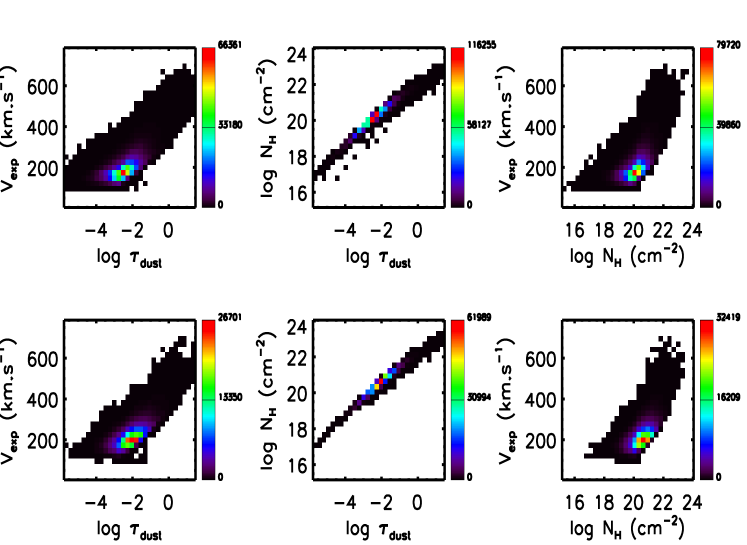
Figure 2: Correlations between the three shell parameters at z $=3.1$ (upper panels) and $4.9$ (lower panels) for the whole sample of galaxies. The expansion velocity $V_{\rm exp}$ is in km.s^-1 and the Hi column density in cm^-2. $\tau_{\rm dust}$ is the dust opacity evaluated at 1216 Å. The colour code scales with the number of objects in each pixel.

Finally, we compute the shell’s dust optical depth at $1216$ Å using Eq. 2. Note that the models for the Hi column density and dust opacity are identical for the Ly$\alpha$ and the UV continuum calculations. This implies that the continuum extinction seen in the spectra from the MCLya library matches the extinction that we apply to our galaxy SEDs. This match allows us to build full spectra for each model galaxy, and to measure the Ly$\alpha$ equivalent width directly as:

$${\rm EW}_{\rm Ly\alpha}=\int\frac{{\rm S}(\lambda)-{\rm C}_{\rm ext}(\lambda)}{{\rm C}_{\rm ext}(\lambda)}d\lambda,$$ (11)

where ${\rm S}$ is defined in Eq. 8 and ${\rm C}_{\rm ext}$ is the extinguished stellar continuum.

3.2.3 Shell parameters distributions

In Figure 2, we show our predicted distributions of the three shell parameters at z $=3.1$ and $4.9$ (they are similar at other redshifts). These quantities show expected correlations. First, there is a tight positive correlation between $N_{\rm H}$ and $\tau_{\rm dust}$, which directly results from our assumption that $\tau_{\rm dust}\propto N_{\rm H}$ in Eq. 2. The small scatter accross this relation is due to metallicity. Second, the shell velocity is a (weak) function of the SFR. Galaxies with more active star formation have a larger reservoir of cold gas, and hence faster shells are also those with higher Hi column densities. The linear relation between $N_{\rm H}$ and $\tau_{\rm dust}$ is responsible for the similar behaviour in the $V_{\rm exp}$-$N_{\rm H}$ and $V_{\rm exp}$-$\tau_{\rm dust}$ planes.

At all z, the Hi column density goes from $\sim 10^{16}$ to a bit less than $10^{24}$ cm^-2. The most probable value of $N_{\rm H}$ is $\sim 10^{20}$ ($5\times 10^{20}$) cm^-2 at z $=3.1$ ($4.9$). The shell velocity distributions span a whole range of values from a few tens to $650$ km.s^-1. Most of the galaxies have $V_{\rm exp}\sim 150-200$ km.s^-1 which is consistent with the z $=3$ sample of LBGs observed by Shapley et al. (2003). The dust opacity of the shells ranges from ${\rm log}(\tau_{\rm dust})=-5$ to $\sim 1.5$. The peak of the distribution shifts from $-2.5$ at z $=3.1$ to $-2$ at z $=4.9$.

3.3 Other models for Ly$\alpha$ Emitters

For discussion, we present here a selection of alternative models taken from the litterature.

3.3.1 Constant $f_{\rm esc}$ model

The so-called constant Ly$\alpha$ escape fraction model, assumes a unique escape fraction of Ly$\alpha$ photons for all galaxies. Using such a model, Le Delliou et al. (2006) fit the Ly$\alpha$ LF data from z $=3.3$ to $6.55$ with a single value $f_{\rm esc}=0.02$. On the other hand, Nagamine et al. (2010) obtain a reasonable fit to the data by varying $f_{\rm esc}$ with redshift, from $0.10$ at $z=3$, to $0.15$ at $z=6$.

Here, we chose a value of $f_{esc}=0.20$, which allows us to reproduce intermediate luminosity counts of the Ly$\alpha$ luminosity function at $z=3.1$. This is also the largest value for our model not to over-predict the bright end of the LF.

For comparison, we also explore the extreme model in which all the Ly$\alpha$ photons are allowed to escape the galaxies, i.e $f_{\rm esc}=1$. In the next sections, we will refer to this model as the no extinction model.

3.3.2 Screen model

In the screen model, the fraction of Ly$\alpha$ photons that escape the galaxy is given by

$$f_{\rm esc}=e^{\rm-\tau_{\rm dust}},$$ (12)

where $\tau_{\rm dust}$ is the dust opacity of the shell. This means that the Ly$\alpha$ line is treated as a normal (non-resonant) radiation, Ly$\alpha$ photons see a screen of gas mixed with dust along their path. A similar model has been investigated by Kobayashi et al. (2007) and Mao et al. (2007) but these authors introduced an additional (free) parameter to reproduce the Ly$\alpha$ LF data.

3.3.3 Slab model

The slab model (Kobayashi et al., 2007), in which the escape fraction is:

$$f_{\rm esc}=\frac{(1-e^{\rm-\tau_{\rm dust}})}{\tau_{\rm dust}},$$ (13)

is similar to the screen model, except that it assumes sources are no longer behind a screen, but uniformly distributed within a slab of gas mixed with dust. Again, and in contrast with us, Kobayashi et al. (2007, 2010) multiplied the above $f_{\rm esc}$ with a constant escape fraction f₀. These authors specify that this constant parameter f₀ takes into account the resonant scattering effect of Ly$\alpha$ photons, the escape of ionizing photons and the IGM transmission.

4 Predicted Ly$\alpha$ escape fractions and Ly$\alpha$ Luminosity Functions

One of the strengths of our fiducial model is that it predicts the Ly$\alpha$ escape fraction of each individual galaxy, as a function of its physical properties. In this section, we first discuss our predicted Ly$\alpha$ escape fraction distribution. Then, we compare our predicted Ly$\alpha$ LFs to observational estimates. We continue with discussions on the equivalent width selection effects and IGM attenuation.

4.1 Distribution of Ly$\alpha$ escape fractions

In Figure 3, we show the distribution of $f_{\rm esc}$ for galaxies in different SFR bins, at z $=3.1$ (thick curves) and z $=4.9$ (thin curves).

A first point illustrated by Figure 3 is that our model predicts a very strong variation of the escape fraction distribution with star formation rate (or, equivalently, with stellar mass). We see that galaxies with high SFRs have a rather uniform $f_{\rm esc}$ distribution (solid black curves), while low-SFR objects let almost all Ly$\alpha$ photons escape (dashed green curves). The main quantity responsible for the flat distribution of the escape fraction for high-SFR galaxies is dust opacity. Galaxies with SFR $>20{\rm M}_{\odot}.{\rm yr}^{-1}$ span a $\tau_{\rm dust}$ range going from $10^{-2}$ to more than $10$, as a consequence of their different star formation and merging histories. Low-SFR objects contain little metal and Hi gas. Consequently, their optical thicknesses are low, and their escape fractions high.

We find that the average (median) escape fraction for galaxies with SFR $>10$M_⊙.yr^-1 is 21% (8%). This compares nicely to the value of 20% we used to fit our constant Ly$\alpha$ escape fraction model at intermediate Ly$\alpha$ luminosity ($10^{42}<L_{\rm Ly\alpha}<10^{43}$erg.s^-1).

A second point we wish to make from Figure 3 is that the distribution of escape fractions, in a given SFR bin, remains almost constant with redshift. The fraction of galaxies per SFR bin does not change significatively between z $=3$ and $5$, because, from Eq. 1, the variations (that is, a decrease with increasing redshift) of cold gas mass and disc radius balance one another. In a given SFR bin, the values of Hi column density and dust opacity (Eq. 10 and 2) remain rather similar over this redshift interval, as a result of the co-evolution of cold gas mass, disc radius and metallicity. This yields the apparent non-redshift-evolution of Figure 3.

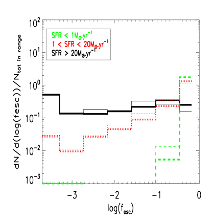
Figure 3: Distribution of Ly$\alpha$ escape fraction at $z\sim 3$ (thick line) and $5$ (thin line). The black solid line refers to galaxies having ${\rm SFR}>20{\rm M}_{\odot}.{\rm yr}^{-1}$, the red dotted line to $1<SFR<20{\rm M}_{\odot}.{\rm yr}^{-1}$ and the green dashed one to low-SFR objects (SFR $<1{\rm M}_{\odot}.{\rm yr}^{-1}$). Low-SFR galaxies have high Ly$\alpha$ escape fractions whereas in intensely star-forming objects, $f_{\rm esc}$ is distributed between $0$ and $1$.

4.2 Ly$\alpha$ luminosity functions

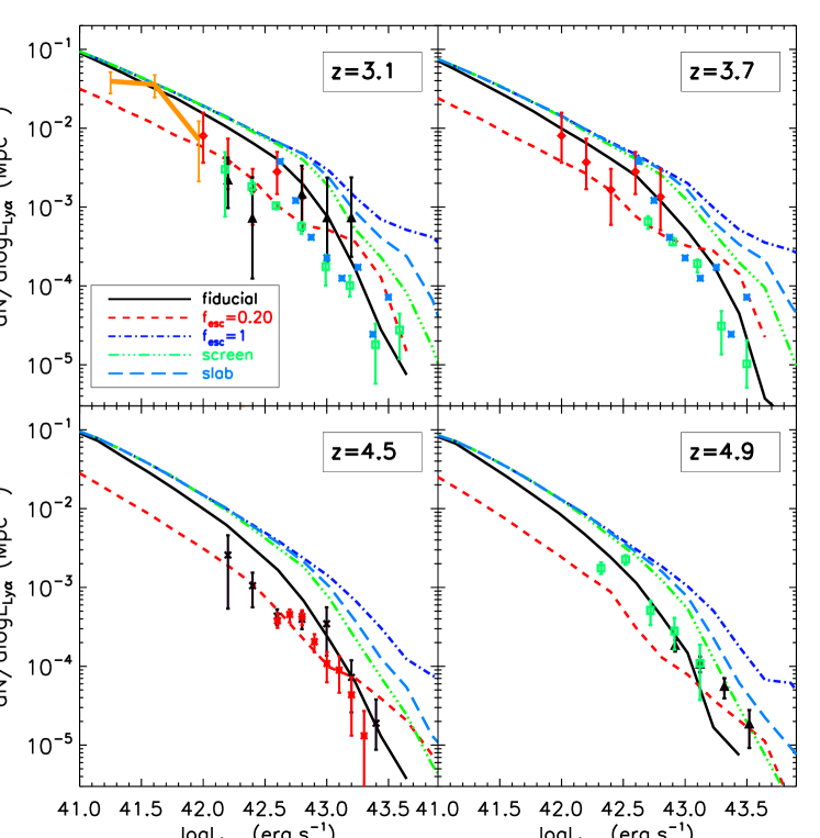
Figure 4: Ly$\alpha$ LFs at z $=3.1,3.7,4.5$ and $4.9$. Black solid line: fiducial model. Red short dashed line: $f_{\rm esc}=0.20$. Blue long dashed line: slab model. Violet dot-dashed line: $f_{\rm esc}=1$. Green dot-dot-dashed line: Screen model. The data points are from van Breukelen et al. (2005) (red diamonds, $2.3<z<4.6$), Kudritzki et al. (2000) (black triangles, z $=3.1$), Ouchi et al. (2008) (green squares, z $=3.1$, $3.7$), Blanc et al. (2010) (blue asterisks, $2.8<z<3.8$), Dawson et al. (2007) (black crosses, z $=4.5$), Wang et al. (2009) (red asterisks, z $=4.5$), Ouchi et al. (2003) (green squares, z $=4.9$) and Shioya et al. (2009) (black triangles, z $=4.9$). The orange line is the observation of Rauch et al. (2008) ($2.67<z<3.75$).

In Figure 4, we show the observed Ly$\alpha$ luminosity functions from $z=3.1$ to $z=4.9$, and compare them to our model (solid black curves). Our model shows a very satisfactory agreement with the observational data over the whole redshift range. Interestingly, it fits as well the bright end ($L_{\rm Ly\alpha}>10^{42}$erg.s^-1) and the faint LAE population observed by Rauch et al. (2008) at z $\sim 3$. This is a direct result of our predicted escape fraction distribution. On the one hand, low-SFR galaxies have $f_{\rm esc}\sim 1$ due to their low dust opacities, which allows us to reproduce the faint counts of Rauch et al. (2008). On the other hand, high-SFR galaxies have a flat distribution of $f_{\rm esc}$, which yields the exponential cutoff at the bright end of the LF, as most of them have a very low escape fraction.

We note that, at z $=3.1$, our model agrees better with spectroscopic observations (Blanc et al., 2010; Rauch et al., 2008; van Breukelen et al., 2005; Kudritzki et al., 2000) than with narrow-band data from Ouchi et al. (2008). We will come back to this issue in Sec. 4.3.

Figure 4 also shows predictions of the other models discussed in Sec. 3.3: the blue dot-dashed (red dashed) curves show predictions from the $f_{\rm esc}=1$ ($f_{\rm esc}=0.20$) model, the blue long-dashed (green 3-dot-dashed) curves show predictions from the slab (screen) models. Interestingly, most models (all except the $f_{\rm esc}=0.20$ one) converge to the same faint-end prediction, consistent with $f_{\rm esc}\sim 1$ for low-mass galaxies. Only our model, though, manages to also reproduce the bright-end, due to its resonant scattering enhancing Ly$\alpha$ absorption in massive, dusty, galaxies.

At the faint end of the Ly$\alpha$ LFs where $f_{\rm esc}\sim 1$, the Ly$\alpha$ luminosity could provide information about the SFR of low mass galaxies, assuming a standard conversion law (Kennicutt, 1998; Furlanetto et al., 2005).

4.3 Selection effects

Let’s note that data from Ouchi et al. (2008) (which represents the largest sample of LAEs) around log($L_{\rm Ly\alpha}$)$\sim 42.1-42.8$ are a bit overestimated by our model. The theoretical Ly$\alpha$ LFs presented in Figure 4 do not contain any kind of selection effect. However, when selected through narrow-band searches, as in Ouchi et al. (2008), observations are subject to a threshold in terms of Ly$\alpha$ equivalent width (EW). Ouchi et al. (2008), especially, have a relatively high threshold at z $=3.1$ (EW${}^{\rm thresh}~{}\sim~{}64$ Å). Since our model is able to predict the emergent Ly$\alpha$ EW of LAEs, we can reproduce such a selection and investigate its impact on LFs estimates.

In Figure 5, we focus on the Ly$\alpha$ LF at $z=3.1$ and show how it varies when selecting galaxies with increasing EWs. The solid curve is the same as in Figure 4 (no selection), the dotted (dashed, dot-dashed) curves correspond to cuts at 35Å (50Å, 64Å). Figure 5 shows that a selection on equivalent width affects the LF at all luminosities, in a rather uniform way. Even at low luminosities ($<10^{41}$erg.s^-1), our model galaxies have a distribution of EWs peaking at around $\sim 65$Å, and are thus affected by drastic EW cuts.

When using the threshold value of 64Å quoted by Ouchi et al. (2008) at face value, we find that our model under-predicts the number density of LAEs observed by these authors (green open squares in Figure 5). Instead, we find good agreement with their LF when applying a cut at $\sim 50$Å. We believe this discrepancy has two causes: (i) our distribution of predicted EWs is perhaps centered at too low values, and (ii) there is a rather large uncertainty in the estimated value of the effective EW cut from these authors’ survey. We discuss our predictions for EWs again in Sec. 5.1.

We learn from this study that narrow-band observations may underestimate the actual number density of LAEs at all luminosities, by a factor ranging from 5 at the bright end to $\sim 2$ at the very faint end ($L\sim 10^{41}$erg.s^-1). Spectroscopic surveys, which are much less sensitive to EW thresholds, are more efficient to detect the whole sample of LAEs. Indeed, it can be seen from Figure 4 that most data points obtained by spectroscopy (Kudritzki et al., 2000; Blanc et al., 2010; van Breukelen et al., 2005) are most of the time above Ouchi et al. (2008) observations, and in better agreement with our model predictions. However, comparing with Gronwall et al. (2007)’s data (who have a much lower EW limit, i.e $20$ Å) does not lead to the same conclusion. Gronwall et al. (2007)’s data (blue dashed line) are very close to those from Ouchi et al. (2008). Applying the $20$ Å to our fiducial model does not reproduce their observed Ly$\alpha$ LF. Understanding why both Ouchi et al. (2008) (sample of 356 objects) and Gronwall et al. (2007) (sample of 162 objects) give a very similar luminosity function at z $=3.1$ in spite of quite different EW limits is not straightforward, given that the number of LAEs detected with EW $<64$ Å is not negligible (Finkelstein et al., 2007; Gronwall et al., 2007). It may be a cosmic variance effect.

In the next paragraph, we discuss what limitations arise from spectroscopic observations we have compared our model with and for which our Ly$\alpha$ LF shows a better match than with narrow-band data.

Observations of Kudritzki et al. (2000) were carried out with slit spectroscopy over $\sim 50$ arcmin² so that their results may be biased by flux losses and cosmic variance. Low redshift interlopers may also have been identified as LAEs. Blanc et al. (2010) apply a $20$ Å equivalent width cut to remove OII emitters from their sample. According to our figure 5, such a low EW threshold should remove a small fraction of LAEs only. Integral field spectroscopy data from van Breukelen et al. (2005) cannot distinguish OII emitters so that their sample of LAEs may be considered as a maximal sample. They argue that $2$ LAEs from their sample could be OII emitters. We did the test of removing those two objects which lie in the two brighter bins of their LF. We found that our model is still in good agreement with these two points even after this correction. Nevertheless, the field of view of van Breukelen et al. (2005) is rather small ($\sim 1.4$ arcmin²) and their data may suffer of cosmic variance effects. A more detailed discussion on pros and cons of narrow-band techniques versus integral field spectroscopy or slit spectroscopy is postponed to a future study (Garel et al., in prep).

Finally, we note that EW limits of narrow-band surveys have a decreasing effect with redshift (see Table 3), so that the number of objects found with narrow-band and spectroscopic techniques should converge at higher redshifts.

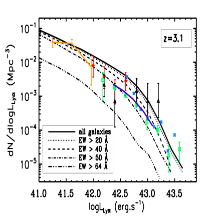
Figure 5: Impact of a Ly$\alpha$ EW threshold on the Ly$\alpha$ LF at z $=3.1$. We plot five LFs with different cuts in Ly$\alpha$ EW. Solid line: no cut. Dotted line: EW${}^{\rm thresh}>20$ Å. Dashed line: EW${}^{\rm thresh}>35$ Å. Dot-Dot-dashed line: EW${}^{\rm thresh}>50$ Å. Dot-dashed line: EW${}^{\rm thresh}>64$ Å. Data points are the same as in Figure 4. Gronwall et al. (2007)’s data are shown as a thick violet line.

4.4 Effect of the IGM

In the results presented so far, we have not included the effect of IGM transmission. However, photons shortwards $1216$Å may be scattered off the line of sight by intergalactic hydrogen atoms. We model this effect as Madau (1995), and define the IGM optical depth as:

$$\tau_{\rm IGM}^{\rm Ly\alpha}=0.0036(\frac{\lambda_{\rm obs}}{\lambda_{\alpha}})^{3.46},$$ (14)

where $\lambda_{\rm obs}=(1+z)\lambda$ is the observer-frame wavelength.

We apply the IGM transmission $T_{\rm IGM}^{\rm Ly\alpha}=e^{\rm-\tau_{\rm IGM}^{\rm Ly\alpha}}$ to the blue part of our spectra, only in the fiducial model (in which we build the emergent Ly$\alpha$ spectra) and in the no extinction model (where we assume the spectrum is unchanged compared to the Gaussian intrinsic spectrum). Other models do not produce spectra and so we discard them here. Note that if one assumes that the f${}_{\rm esc}=0.20$ model does not affect the line shape but only its amplitude, it would undergo exactly the same IGM attenuation as the no extinction model does.

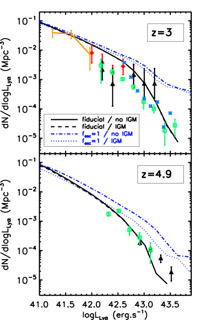
Figure 6: Comparison of the Ly$\alpha$ LFs at z $=3.1$ and $4.9$ with and without IGM transmission. The behaviour is similar at z $=3.7$ and $4.5$. Black solid line: fiducial model without IGM. Black dashed line: fiducial model with IGM. Violet dot-dashed line: No extinction model without IGM. Violet dotted line: No extinction model with IGM. Note that a horizontal shift of log(0.20) of the violet curve gives the f${}_{\rm esc}=0.20$ model in the assumption that the line shape is unchanged by shell transfer effects. Data points are the same as in Figure 4.

In Figure 6, we show how the IGM transmission affects the Ly$\alpha$ LF at $3.1$ and $4.9$ only since the results at z $=3.7$ and $4.5$ lead to the same conclusions we discuss below. We find that the IGM has a negligible impact on our model’s Ly$\alpha$ LFs. This is due to the fact that, in this model, most of the galaxies’ spectra have P-Cygni profiles, with a redward peak in emission and a deep absorption on the blue side. As our model for IGM transmission only applies to the blue side of the spectra, we indeed expect little effect from the IGM. This is probably a good approximation in most cases where the IGM does not produce any damped absorption line which could leak redwards of the Ly$\alpha$ line. The fact that the attenuation of Ly$\alpha$ by the IGM may be relatively small or even negligible in case of outflows has already been noted by several authors, including e.g. Haiman (2002); Santos et al. (2004); Verhamme et al. (2008); Dijkstra & Wyithe (2010) and others. In the no extinction model, we have assumed the spectra emerging from the galaxy are Gaussian. In this case, the transmission through the IGM has a clear effect on the LF: it reduces luminosities by a factor $\sim 2$ at z $=5$. This is not enough, however, to bring this model in agreement with the data at z $\leq 5$, which suggests that IGM attenuation alone cannot explain the observations.

5 Properties of Ly$\alpha$ Emitters

We now study in more detail the properties of LAEs at $3<z<5$ as predicted by our fiducial model, and we compare them to other available data.

5.1 Ly$\alpha$ equivalent width

In this section, we present the rest-frame intrinsic Ly$\alpha$ EWs obtained from Eq. 7, and the rest-frame emergent (after radiation transfer) Ly$\alpha$ EWs predicted by our fiducial model from Eq. 11.

In Figure 7, we compare our predicted Ly$\alpha$ EW distributions with observations at various redshifts (z $=3.1,3.7,4.5$ and $4.9$). To perform a reliable comparison, we apply the same criteria in terms of Ly$\alpha$ luminosity and EW cuts as in each dataset (see Table 3). In each panel, we show three histograms. The dotted green curve represents the raw distribution of intrinsic Ly$\alpha$ EWs. The peak is at $65-70$ Å at all redshifts, with very few objects having high Ly$\alpha$ EWs ($>100$ Å). The first reason of the deficit of high Ly$\alpha$ EWs, and of the absence of very high Ly$\alpha$ EWs ($>200$ Å) may be the absence of star formation bursts in our GALICS galaxies. Indeed, as gas accretion is a continuous and smooth process, the SFRs evolve smoothly and no galaxies show very short timescale bursts able to enhance the Ly$\alpha$ EW. Galaxies displaying a constant SFR have rather low Ly$\alpha$ EWs (Charlot & Fall, 1993). Another reason for our lack of high EWs may be that we use a Kennicutt IMF. Considering a shallower IMF, or a higher high-mass cutoff could enhance the intrinsic Ly$\alpha$ EWs (Charlot & Fall, 1993). A third reason for the shallow distribution of emergent EWs could be due to large errors in the estimate of EWs. To take into account statistical uncertainties, we have convolved this distribution with a Gaussian ($\sigma=50$ Å), which yields the green dashed curve. The choice of $50$ Å is arbitrary and corresponds to the size of the bin in Figure 7 and in the Ly$\alpha$ EWs distributions commonly presented by observers. We assume that the dispersion in measurement uncertainties should not exceed this value (though it is hard to quantify). Even with this ’high’ $\sigma$ value, we do not reach very high intrinsic Ly$\alpha$ EWs ($>200$ Å).

We do not show the raw distribution of emergent Ly$\alpha$ EWs obtained with our model for the sake of clarity. At z $=3.1-3.7$, it is hardly distinguishable from the intrinsic distribution. At z $=4.5-4.9$, the peak would be shifted to the $0-50$ Å bin and the distribution as narrow as the raw distribution. In Figure 7, the solid black line represents the distribution of emergent Ly$\alpha$ EWs convolved with a Gaussian ($\sigma=50$ Å), as we did for the intrinsic distribution. We can see that, at z $=3.1,3.7$ and $4.9$, the locations of the peaks of the distributions in our predictions are in agreement with the observations. We should note that, at z $=4.5$, even if the model peak matches the observed distribution from Finkelstein et al. (2007), it is not the case compared with Dawson et al. (2007)’s data. However, if we were comparing this z = $4.5$ model distribution with z = $4.9$ data from Shioya et al. (2009), we would get a good match (Finkelstein et al., 2007; Shioya et al., 2009; Dawson et al., 2007, have nearly the same luminosity and EW detection limits so the same model can compare with these observations). Then, we argue that it is hard to draw conclusions in that case. On the other hand, it is straightforward to conclude that all our distributions are not spread enough compared with any data. We discuss briefly this issue.

The emergent Ly$\alpha$ EWs obtained with our fiducial model are lower than the intrinsic ones which, as discussed above, do not reach large values and have a narrow distribution. Since the amount of dust seen by the continuum and the Ly$\alpha$ line is the same, and given that the Ly$\alpha$ line is resonant (and, consequently, more extinguished), it is impossible for any galaxy to have an emergent Ly$\alpha$ EW greater than the intrinsic one in our model. Only models with clumpy dust distributions (Neufeld, 1991) would allow $EW_{\rm Ly\alpha}>EW_{\rm Ly\alpha}^{\rm intr}$. Despite the lack of large EW systems, we note that our distribution reproduces a significant fraction of observed systems, which is satisfactory.

The reproduction of a shallow Ly$\alpha$ EW distribution with very large Ly$\alpha$ EWs is a puzzling issue for other models too (Samui et al., 2009; Dayal et al., 2008). Dayal et al. (2008) argue that physical effects such as gas kinematics, metallicity, population III stars and young stellar ages could spread the EW distribution, and lead to higher EW values. Kobayashi et al. (2010) are able to retrieve the very large Ly$\alpha$ EWs thanks to the inclusion of both young and low-metallicity stellar populations and clumpy dust in their time-sequence outflow model. The value of their clumpiness parameter (q${}_{\rm d}=0.15=$ clumpy dust) arises from the calculation of both continuum and Ly$\alpha$ dust opacities which are computed from two different ways.

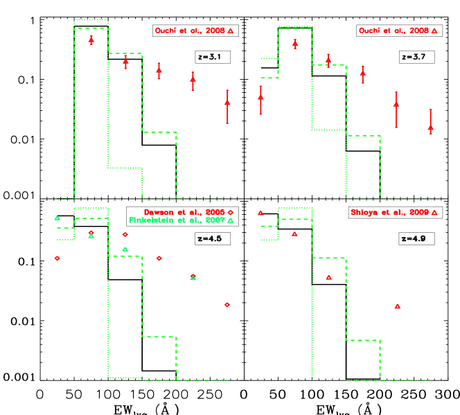
Figure 7: EW distributions at z $=3,3.7,4.5$ and $4.9$. Dotted green line: Raw distribution of intrinsic Ly$\alpha$ EWs. The two other curves have been convolved with a Gaussian ($\sigma=50$ Å) to account for statistical uncertainties. Solid black line: Emergent Ly$\alpha$ EW distribution (fiducial model) with convolution. Dashed green line: Intrinsic Ly$\alpha$ EW distribution with convolution. We apply the same thresholds in terms of Ly$\alpha$ EW and luminosity as each individual set of data as summarized in Table 3.

author	redshift	EWLyα ${}^{\textrm{a}}$ (Å)	$L_{\rm Ly\alpha}$ ${}^{\textrm{b}}$ (erg.s-1)
Ouchi et al. (2008)	z $\sim 3.1$	$64$	$10^{42}$
Gronwall al. (2007)	z $\sim 3.1$	$20$	$1.1\times 10^{42}$
Ouchi et al. (2008)	z $\sim 3.7$	$44$	$4\times 10^{42}$
Dawson et al. (2007)	z $\sim 4.5$	$14$	$4\times 10^{42}$
Finkelstein et al. (2007)	z $\sim 4.5$	$20$	$4\times 10^{42}$
Wang et al. (2009)	z $\sim 4.5$	$14$	$3.5\times 10^{42}$
Ouchi et al. (2003)	z $\sim 4.9$	$14$	$7\times 10^{41}$
Shioya al. (2009)	z $\sim 4.9$	$11$	$3.8\times 10^{42}$

Table 3: Detection limits of narrow-band surveys. a: limiting Ly$\alpha$ rest-frame EW of the survey. b: limiting Ly$\alpha$ luminosity of the survey.

5.2 UV Luminosity Functions of Ly$\alpha$ Emitters

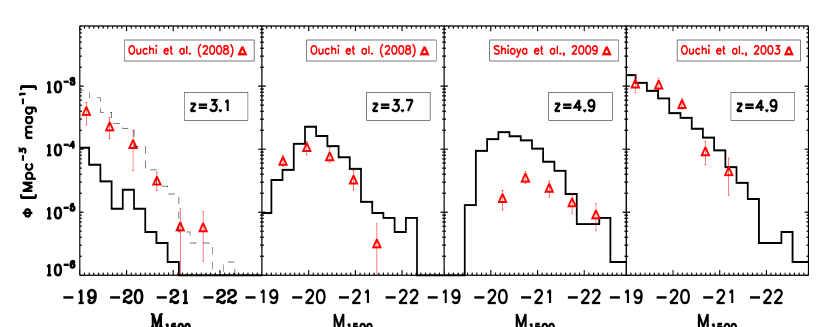
Figure 8: Observed (red symbols) and predicted (black lines) rest-frame UV LFs of LAEs at $1500$ Å. For each LF, we apply the same cuts in Ly$\alpha$ luminosity and EW as in the observations. The dashed line at $z\sim 3.1$ (left panel) shows the model applying a somewhat lower EW threshold of 50 Å.

As noted in Samui et al. (2009), only a fraction of the whole galaxy population is detected as LAEs because of the survey limits (in $L_{\rm Ly\alpha}$ and EW). By applying the same thresholds as in the observations, we compute the UV LFs of LAEs at z $=3.1,3.7$ and $4.9$ with our fiducial model and investigate the relation between UV-selected galaxies (LBGs) and LAEs.

In Figure 8, we show the UV LFs of Ly$\alpha$-selected model galaxies. We find a rather good agreement with observations, especially with Ouchi et al. (2008) at z $=3.7$, and with Ouchi et al. (2003) at z $=4.9$. However, there are two discrepancies we wish to comment on.

As already discussed with Figure 5, the EW limit of Ouchi et al. (2008) at z $=3.1$ ($64$ Å) has a dramatic effect on our model, since we predict very few objects with large EWs. As a consequence, if we reproduce the same EW cut, we again find less LAEs than these authors (solid histogram in left-hand-side panel of Figure 8). To bypass this conflict, we may lower the EW cut we apply to our model until we find the same number density of LAEs. We obtain this match at $\sim$50Å, which is the value we had to apply to our modelled Ly$\alpha$ LF at z $=3.1$ to fit the data from Ouchi et al. (2008). The UV LF of our model galaxies selected in this way is plotted as the dashed curve on Figure 8. The good agreement we find now tells us that, provided we have the same number of objects, we manage to reproduce their UV luminosity distribution.

For other redshifts, the EW thresholds are lower, so that our lack of high EW is no longer a problem. However, our model does not match z $=4.9$ data from Shioya et al. (2009), and we find many more UV-faint objects than they do. The reason of this disagreement is unclear, especially given that our model agrees with data from Ouchi et al. (2003) at the same redshift. This suggests that observations themselves may not agree one set with another and that more data is needed to shed light on this issue.

From this discussion, we conclude that our model is in broad agreement with observed UV properties of LAEs. And we once again demonstrate the special care that needs to be taken to reproduce selection effects.

We may now turn the question the other way around, and ask whether our model reproduces the Ly$\alpha$ properties of UV-selected galaxies. Shapley et al. (2003) studied the Ly$\alpha$ emission of LBGs at z $=3$. They divided their LBG sample into four bins of Ly$\alpha$ EW and found that $\sim$25 % of LBGs have EWs $>20$ Å and $\sim$50 % show Ly$\alpha$ emission (EW $>0$ Å). It is not straightforward to apply the LBG selection to our model galaxies, and even more given the complex selections inherent to spectroscopic followups. Instead, here, we simply apply various rest-frame UV absolute magnitude cuts which should roughly bracket the selection of Shapley et al. (2003). With a selection limit of M${}_{1500}<-21$, we find that 28 % of the selected LBGs have EW $>20$ Å and 69 % display Ly$\alpha$ emission (EW $>0$ Å) at z $=3.1$. Varying our selection limit, we find, for M${}_{1500}<-21.5$ (M${}_{1500}<-20.5$), that 25 % (39 %) of the objects have EW $>20$ Å, and 74 % (71 %) of the selected LBGs are detected in emission. Thus the model predicts 1.75 to 3 times less LBGs with EW $>20$ Å than LBGs simply displaying Ly$\alpha$ emission, whereas Shapley et al. (2003) found a factor of two. The discrepancy with their observations may come from the rest-frame selection instead of apparent magnitude selection, the value of the cut, and maybe the fact that they may have missed the detection of very faint Ly$\alpha$ lines (very low Ly$\alpha$ EW) in their sample.

5.3 Stellar masses of Ly$\alpha$ Emitters

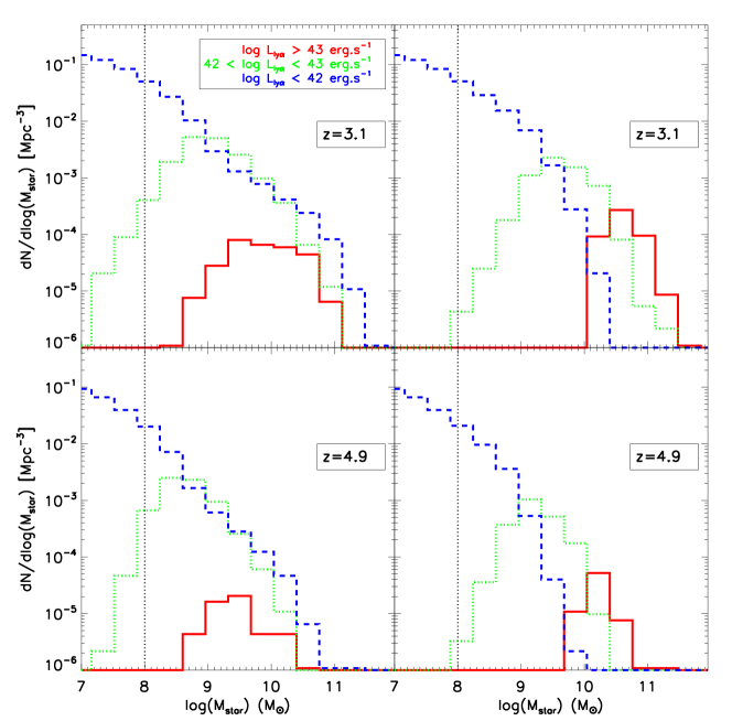
Figure 9: Distribution of the stellar masses divided in three bins of Ly$\alpha$ luminosity at z $=3.1$ (top) and $4.9$ (bottom). In each bin, the number of objects is divided by the bin size and the volume of the box. Solid red line: $L_{\rm Ly\alpha}>10^{43}\mbox{erg.s}^{-1}$. Dotted green line: $10^{42}<L_{\rm Ly\alpha}<10^{43}\mbox{erg.s}^{-1}$. In the left column, we show the fiducial model results. Most massive galaxies are not the brightest LAEs as a consequence of their high dust extinction. The mass ranges spanned by bright LAEs ($L_{\rm Ly\alpha}>10^{42}\mbox{erg.s}^{-1}$, corresponding to currently observed LAEs) broadly agree with observational estimates at various redshifts. In the right column, we present the stellar mass distribution computed from the constant Ly$\alpha$ escape fraction model ($f_{\rm esc}=0.20$), for comparison with our fiducial model. In the constant Ly$\alpha$ escape fraction model, the stellar mass scales with the Ly$\alpha$ luminosity which predicts higher masses than what is observationally derived. The mass resolution effect of the simulation starts playing a role in the stellar mass distributions at $\sim 10^{8}$ M_⊙ (vertical dotted line in each panel).

Figure 9 plots the stellar mass distributions of LAEs divided into three Ly$\alpha$ luminosity bins at z $=3.1$ and $4.9$. Stellar mass distributions slowly shift to lower stellar masses by increasing the redshift. At intermediate redshifts, the results show the same behaviour as those at z $=3.1$ and $4.9$ so we do not show them here.

We compare the results of our fiducial model (left column) and the $f_{\rm esc}=0.20$ model (right column). As expected, in the latter model, brightest LAEs ($L_{\rm Ly\alpha}>10^{43}\mbox{erg.s}^{-1}$) have higher stellar masses, and fainter LAEs are less massive objects. It is expected since Ly$\alpha$ luminosities scale with SFRs which is tightly correlated to stellar mass at these redshifts. In our fiducial model, however, the behaviour is slightly different. If high Ly$\alpha$ luminosity objects have medium and rather large stellar masses (from $10^{8}$ to $10^{11}$ M_⊙), the most massive objects ($>10^{11}$ M_⊙) are faint LAEs ($L_{\rm Ly\alpha}<10^{41}\mbox{erg.s}^{-1}$). This is a consequence of the nearly flat Ly$\alpha$ escape fraction distribution that we find for high SFR (massive) objects (Figure 3). For the largest fraction of LAEs which are currently observed ($L_{\rm Ly\alpha}>10^{42}\mbox{erg.s}^{-1}$), we predict stellar masses ranging from $10^{7}$ to $10^{11}$ M_⊙.

At z $=3.1$, Gawiser et al. (2006) find a mean stellar mass of $5.10^{8}$ M_⊙ which agrees with the mean value predicted by our fiducial model for LAEs in the range $10^{42}<L_{\rm Ly\alpha}<10^{43}\mbox{erg.s}^{-1}$. The constant Ly$\alpha$ escape fraction model predicts, however, a mean value almost ten times higher for this luminosity range.

Massive LAEs ($10^{10-11}$M_⊙) recently observed at z $=3-4$ by Ono et al. (2010) have Ly$\alpha$ luminosties comprised between $\sim 10^{42}$ and $2\times 10^{43}\mbox{erg.s}^{-1}$. Those more massive galaxies fit in the range of prediction of our model (green and red curves of the top left panel of Figure 9).

LAEs reported by Finkelstein et al. (2007) at z $=4.5$ have stellar masses ranging from $2.10^{7}$ to $2.10^{9}$ M_⊙. For $L_{\rm Ly\alpha}>10^{42}\mbox{erg.s}^{-1}$, the fiducial model yields a mass range from $2.10^{7}$ to $2.10^{10}$ M_⊙, whereas the constant Ly$\alpha$ escape fraction model predicts higher masses.

Pirzkal et al. (2007) observed LAEs with $L_{\rm Ly\alpha}>2.10^{42}\mbox{erg.s}^{-1}$ having $10^{7}<M_{\rm star}<2.10^{9}$ M_⊙ at z $\sim 5$, which is rather similar to the results obtained from the fiducial model at z $=4.9$, and below the interval spanned by the constant Ly$\alpha$ escape fraction model.

Therefore, in the redshift range $3<z<5$, our model gives stellar masses for bright LAEs ($L_{\rm Ly\alpha}>10^{42}\mbox{erg.s}^{-1}$) closer to what is observed than the constant Ly$\alpha$ escape fraction model, and naturally recovers the observational fact that LAEs which are currently observed are not very massive objects.

5.4 Ando effect

Many authors reported a deficit of high Ly$\alpha$ EW ($>100$ Å) in UV bright objects (M${}_{1500}<-22$) between z $=3$ and $6$ (Ando et al., 2006; Shimasaku et al., 2006; Ouchi et al., 2008; Stark et al., 2010). We will refer to this effect as the Ando effect. It has also been discussed in theoretical papers (Verhamme et al., 2008; Kobayashi et al., 2010). The reasons invoked to explain this effect are multiple: the time-sequence of a starburst, resonant scattering in the gas, a clumpy dust distribution and/or the age of the stellar population. We investigate this feature with our model and plot our results in Figure 10. We find that we recover this effect at $3<z<5$. Since our model does not reproduce very accurately the observed Ly$\alpha$ EW, we do not compare with observational data, but we only discuss the effect qualitatively.

To see why our model predicts this lack of high Ly$\alpha$ EW in UV bright galaxies, we show the relation between the dust-uncorrected UV magnitude, and the intrinsic Ly$\alpha$ EW in Figure 11. There is almost no correlation between those two quantities, except that the highest intrinsic Ly$\alpha$ EWs come from UV faint galaxies. It is due to the fact that UV bright objects have old stellar populations, whereas fainter galaxies display a whole range of ages. A fraction of the UV-faint objects are young, so that they have a high ratio of ionizing luminosity over UV-continuum luminosity $L_{\lambda<912}/L_{\rm cont}$ which produces large intrinsic Ly$\alpha$ EWs. This ratio is, on average, smaller for older, UV-brighter galaxies, so that large intrinsic Ly$\alpha$ EWs do not exist for those objects. From this study of the galaxy SEDs, we are able to find part of the explanation of the absence of high Ly$\alpha$ EWs among UV-bright objects.

Looking again at Figure 10, we can see that this lack is more significant for the observed Ly$\alpha$ EW (after radiative transfer) than in the M${}_{1500}^{\rm uncorr}$-EW${}_{Ly\alpha}^{\rm intr}$ plane (Figure 11). In our model, Hi column densities (and dust opacities, by construction of the dust opacity in our model) take large values for UV-bright galaxies, as shown by Figure 12. We then argue that, in those galaxies, Ly$\alpha$ photons are more extinguished than in UV-faint galaxies, because of the resonance of the Ly$\alpha$ line in a dense, dusty medium.

As we do not reproduce the observed distribution of Ly$\alpha$ EWs at high values ($>150$ Å), we have to be prudent with our conclusions. We can wonder what would be the impact of the physical effects that we identified as a possible explanation for very large Ly$\alpha$ EWs on the Ando effect. Would clumpiness and resolved starbursts (young stellar populations) lead to high Ly$\alpha$ EW values in UV bright or faint galaxies preferentially? A possible answer can be inferred from Kobayashi et al. (2010). They find that these two effects lead to smaller (larger) Ly$\alpha$ EWs in UV brighter (fainter) galaxies. Then, the no-reproduction of large Ly$\alpha$ EWs in our model should not impact our interpretation of the Ando effect.

Therefore, we find two main reasons to explain the Ando effect in our model: (i) UV-bright galaxies are old, so that they do not show high intrinsic Ly$\alpha$ EWs, and (ii) Hi column densities for UV-bright objects are larger, which leads to an enhanced destruction of Ly$\alpha$ photons as a consequence of radiation transfer effects, as already suggested by Verhamme et al. (2008).

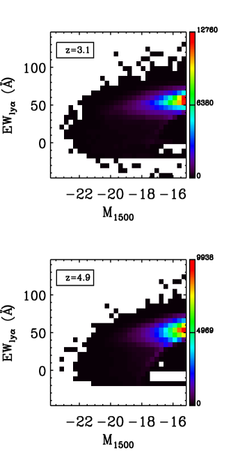
Figure 10: Observed Ly$\alpha$ EW versus the UV magnitude at 1500 Å for the fiducial model at z $=3.1$ and $4.9$. The colour of each pixel represent the number of objects in that pixel.

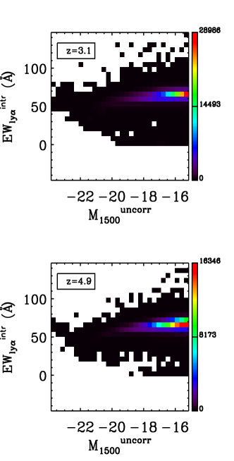
Figure 11: Intrinsic Ly$\alpha$ EW versus the dust-uncorrected UV magnitude at $1500$ Å for the fiducial model at z $=3.1$ and $4.9$. The colour of each pixel represent the number of objects in that pixel.

Figure 12: Hi shell column density versus the UV magnitude at 1500 Å for the fiducial model at z $=$ 3.1 and 4.9. The colour of each pixel represent the number of objects in that pixel. The no-data area (white hole) at M₁₅₀₀ $\sim$ 16 and log$(N_{\rm H})\sim$ 22 is due to the fact that (i) log$(N_{\rm H})$ is correlated to the dust-uncorrected magnitude M${}_{1500}^{\rm uncorr}$ (both proportional to the galaxy mass), and (ii) $\tau_{\rm dust}$ is proportional to N_H (Eq. 2). This implies that intrinsically bright UV galaxies, in our model, have large log$(N_{\rm H})$ values and are strongly extinguished, in terms of UV magnitude, by $\sim-2.5\times log(exp(-\tau_{\rm dust}))\sim\tau_{\rm dust}\propto N_{\rm H}$. This makes the rightward shift of large log$(N_{\rm H})$ points in this figure.

6 Discussion and conclusions

In this paper, we have presented a new semi-analytic model for high redshift LAEs. We have investigated the Ly$\alpha$ emission and transfer processes taking into account resonant scattering effects through gas outflows. To this aim, we have coupled the output of the GALICS semi-analytic model with results of Monte-Carlo radiation transfer runs which compute the Ly$\alpha$ transfer through static and expanding shells. We had to make a few simplifying assumptions (central emission, sphericity and homogeneity of the shell), and to use relations for the expanding shell that scale with the physical properties of the galaxies as they are computed by the semi-analytic model.

We have run this new model on a high-resolution N-body simulation ($1024^{3}$ particles) of a large cosmological volume (V$=(100$h${}^{-1})^{3}$ Mpc³) of dark matter. Then, we have enough statistics for massive, rare objects, and enough resolution for less massive objects ($M_{\rm halo}^{\rm min}=1.70\times 10^{9}$ M_⊙). In this first paper, we aim at getting a coherent view of LAEs. We fit the UV LF at z $=3-5$ on a compilation of available data (Figure 1) by adopting a high normalization of the SFR, that, in any case, scales with gas mass as in Kennicutt’s local relation. Then, we get the following results:

• The Ly$\alpha$ escape fraction for each galaxy is obtained by taking into account the resonant nature of the Ly$\alpha$ line. This is in sharp contrast with the assumptions made in previous semi-analytical models. The distribution of $f_{\rm esc}$ is broad, and we see a trend with stellar masses of galaxies (Figure 3). Low-mass galaxies have $f_{\rm esc}$ of the order of unity, and massive galaxies span a broad range of $f_{\rm esc}$ values.

• Because of this trend, the resulting Ly$\alpha$ LFs are steeper from bright to faint luminosities than observed in simpler toy models (constant Ly$\alpha$ escape fraction, screen and slab).

• Ly$\alpha$ LFs are well reproduced between z $=3$ and $5$ (Figure 4) without any additional free parameter in the Ly$\alpha$ model. More specifically, low-luminosity data from Rauch et al. (2008) at z $\sim 3$ are reproduced, so that we predict more faint LAEs than commonly used constant Ly$\alpha$ escape fraction models.

• We have shown that Ly$\alpha$ LFs are sensitive to Ly$\alpha$ EW cuts (Figure 5). This may explain the scatter in the compilation of data, since surveys (both spectroscopic and narrow-band) are subject to different Ly$\alpha$ EW selection limits.

• The IGM attenuation of Ly$\alpha$ photons is very weak in our model, because the predicted Ly$\alpha$ spectra are redshifted with respect to the Ly$\alpha$ line center, as a consequence of the scatter of Ly$\alpha$ photons in the expanding shell (Figure 6). Therefore, in our model, the Ly$\alpha$ transfer within the shell alone explains the observed luminosities of LAEs.

• The predicted distributions of Ly$\alpha$ EWs are narrower than the data (Figure 7). About 85 % of the observed samples have $0<{\rm EW}<150$ Å, and can roughly be reproduced by the model. However, we predict very few objects with EW $>150$ Å, whereas some are observed. Effects that are not included in the model, like short bursts of star formation, a top-heavy IMF, population III stars and/or dust clumpiness, may be the cause of such high Ly$\alpha$ EWs. On the other hand, even without invoking such processes, our fiducial model is able to recover roughly the bulk of the EW distribution.

• The UV LFs of LAEs are in agreement with most data, with some discrepancies (Figure 8). The scatter in the data may be due to poorly-controlled selection criteria.

• We find that our predictions of the fraction of Ly$\alpha$ emitting LBGs follow the same trend as the one found by Shapley et al. (2003), that is to say, $\sim 2$ times less LBGs having EW $>20$ Å than LBGs having EW $>0$ Å. However, our LBG selection (in rest-frame magnitude) is somehow arbitrary since, in this study, we do not attempt to take into account the apparent colors and magnitudes that are necessary to select LBGs correctly.

• Whereas in a simple constant Ly$\alpha$ escape fraction model, Ly$\alpha$ luminosities scale with stellar masses, we find that most massive objects are faint LAEs (Figure 9). Our predicted stellar masses for rather bright LAEs are in correct agreement with observational estimates which find that LAEs are intermediate-mass objects.

• The deficit of high Ly$\alpha$ EWs (the Ando effect) that is found in UV-bright galaxies is well reproduced by our model (Figure 10). The absence of such large Ly$\alpha$ EWs comes from the fact that Hi column densities are high for UV-bright objects, which preferentially extinguishes Ly$\alpha$ photons, as already suggested by Verhamme et al. (2008). Moreover, UV-bright (and consequently massive) galaxies host older stellar populations which prevent them from having high intrinsic Ly$\alpha$ EWs.

In spite of some discrepancies with specific data sets, the overall picture seems to be quite satisfactory, given the crudeness of the assumptions. Most of the observational constraints on high redshift LAEs are well recovered by our model.

Although the coupling of the semi-analytic model with Ly$\alpha$ radiation transfer is admittedly very crude, our global description seems to catch the intuitive trend according to which fainter galaxies, on an average, are more transparent for Ly$\alpha$ photons.

The hypothesis that gas outflows (with speed from a few tens to hundreds km.s^-1) are common in high redshift galaxies is well supported by observations. With such a model, we have been able to agree with many observational data and we found no need to invoke the influence of gas infalls on the Ly$\alpha$ line. Indeed, it has already been shown that it is hard to recover the redward asymetry of the Ly$\alpha$ line with models of Ly$\alpha$ radiative transfer through infalling neutral gas (Verhamme et al., 2006; Dijkstra et al., 2007).

Obviously more refined models are still necessary, to relax some of the assumptions, especially spherical symmetry and homogeneity of the shell. The cases for more realistic geometries and the effect of galaxy inclination are being investigated (Verhamme et al., 2012).

The simulation we used in this paper has been run with initial conditions in agreement with the WMAP 3 release, in which the $\sigma_{8}$ value is low. Structure growth is delayed with this low normalisation of the power spectrum, and fewer objects form at high redshift. This choice has consequences on our ability to reproduce galaxies beyond z $=6$, and we somehow correct this effect for lower redshifts (3 to 5) by normalizing the SFR parameter in order to fit the UV LFs. New simulations with an up-to-date cosmology (WMAP 5/7), where the derived $\sigma_{8}$ value is larger, can help to investigate higher redshifts with our approach.

Even if the number of detections of LAEs is always increasing, the data are still quite heterogeneous. Forthcoming LAE surveys with the Hobby-Eberly Telescope Dark Energy Experiment (HETDEX, Hill et al., 2008) (z $<3.8$; bright objects only), and the Multi Unit Spectroscopic Explorer (MUSE, Bacon et al., 2006) at the Very Large Telescope ($2.8<z<6.7$) should produce more coherent datasets. In a forthcoming paper (Garel et al., in prep.), we will present predictions for MUSE observations with our model.

7 Acknowledgements

The authors thank Roland Bacon, Steven L. Finkelstein, Léo Michel-Dansac, Johan Richard, Karl Joakim Rosdhal and Christian Tapken for useful comments and discussions. The simulation used in this work was carried out and provided by the Horizon project. The authors also acknowledge support from the the BINGO Project (ANR-08-BLAN-0316-01). DS and MH are supported by the Swiss National Science Foundation.

We thank the anonymous referee for his/her careful reading of the manuscript, and his/her comments and suggestions that have helped the authors improve the paper.

Catalogues containing the model outputs presented in this paper can be available upon request at: thibault.garel@univ-lyon1.fr

References

- Ando et al. (2006) Ando M., Ohta K., Iwata I., Akiyama M., Aoki K., Tamura N., 2006, ApJ, 645, L9
- Arnouts et al. (2005) Arnouts S., Schiminovich D., Ilbert O., Tresse L., Milliard B., Treyer M., Bardelli S., Budavari T., Wyder T. K., Zucca E., Le Fèvre O., Martin D. C., Vettolani G., Adami C., Arnaboldi M., Barlow T., Bianchi L., Bolzonella M., Bottini D., Byun Y., Cappi A., Charlot S., Contini T., Donas J., Forster K., Foucaud S., Franzetti P., Friedman P. G., Garilli B., Gavignaud I., Guzzo L., Heckman T. M., Hoopes C., Iovino A., Jelinsky P., Le Brun V., Lee Y., Maccagni D., Madore B. F., Malina R., Marano B., Marinoni C., McCracken H. J., Mazure A., Meneux B., Merighi R., Morrissey P., Neff S., Paltani S., Pellò R., Picat J. P., Pollo A., Pozzetti L., Radovich M., Rich R. M., Scaramella R., Scodeggio M., Seibert M., Siegmund O., Small T., Szalay A. S., Welsh B., Xu C. K., Zamorani G., Zanichelli A., 2005, ApJ, 619, L43
- Bacon et al. (2006) Bacon R., Bauer S., Böhm P., Boudon D., Brau-Nogue S., Caillier P., Capoani L., Carollo C. M., Champavert N., Contini T., Daguise E., Dalle D., Delabre B., Devriendt J., Dreizler S., Dubois J., Dupieux M., Dupin J., Emsellem E., Ferruit P., Franx M., Gallou G., Gerssen J., Guiderdoni B., Hahn T., Hofmann D., Jarno A., Kelz A., Koehler C., Kollatschny W., Kosmalski J., Laurent F., Lilly S. J., Lizon J., Loupias M., Lynn S., Manescau A., McDermid R. M., Monstein C., Nicklas H., Perès L., Pasquini L., Pécontal E., Pécontal-Rousset A., Pello R., Petit C., Picat J., Popow E., Quirrenbach A., Reiss R., Renault E., Roth M., Schaye J., Soucail G., Steinmetz M., Ströbele S., Stuik R., Weilbacher P., Wozniak H., de Zeeuw P. T., 2006, The Messenger, 124, 5
- Baker et al. (2004) Baker A. J., Tacconi L. J., Genzel R., Lehnert M. D., Lutz D., 2004, ApJ, 604, 125
- Bertone et al. (2005) Bertone S., Stoehr F., White S. D. M., 2005, MNRAS, 359, 1201
- Blaizot et al. (2004) Blaizot J., Guiderdoni B., Devriendt J. E. G., Bouchet F. R., Hatton S. J., Stoehr F., 2004, MNRAS, 352, 571
- Blanc et al. (2010) Blanc G. A., Adams J., Gebhardt K., Hill G. J., Drory N., Hao L., Bender R., Ciardullo R., Finkelstein S. L., Gawiser E., Gronwall C., Hopp U., Jeong D., Kelzenberg R., Komatsu E., MacQueen P., Murphy J. D., Roth M. M., Schneider D. P., Tufts J., 2010, ArXiv e-prints
- Bouwens et al. (2007) Bouwens R. J., Illingworth G. D., Franx M., Ford H., 2007, ApJ, 670, 928
- Cattaneo et al. (2008) Cattaneo A., Dekel A., Faber S. M., Guiderdoni B., 2008, MNRAS, 389, 567
- Charlot & Fall (1993) Charlot S., Fall S. M., 1993, ApJ, 415, 580
- Dawson et al. (2007) Dawson S., Rhoads J. E., Malhotra S., Stern D., Wang J., Dey A., Spinrad H., Jannuzi B. T., 2007, ApJ, 671, 1227
- Dawson et al. (2002) Dawson S., Spinrad H., Stern D., Dey A., van Breugel W., de Vries W., Reuland M., 2002, ApJ, 570, 92
- Dayal et al. (2008) Dayal P., Ferrara A., Gallerani S., 2008, MNRAS, 389, 1683
- Dekel & Birnboim (2006) Dekel A., Birnboim Y., 2006, MNRAS, 368, 2
- Devriendt et al. (1999) Devriendt J. E. G., Guiderdoni B., Sadat R., 1999, A&A, 350, 381
- Dijkstra et al. (2006) Dijkstra M., Haiman Z., Spaans M., 2006, ApJ, 649, 14
- Dijkstra et al. (2007) Dijkstra M., Lidz A., Wyithe J. S. B., 2007, MNRAS, 377, 1175
- Dijkstra & Loeb (2008) Dijkstra M., Loeb A., 2008, MNRAS, 391, 457
- Dijkstra & Wyithe (2010) Dijkstra M., Wyithe J. S. B., 2010, MNRAS, 408, 352
- Finkelstein et al. (2007) Finkelstein S. L., Rhoads J. E., Malhotra S., Pirzkal N., Wang J., 2007, ApJ, 660, 1023
- Furlanetto et al. (2005) Furlanetto S. R., Schaye J., Springel V., Hernquist L., 2005, ApJ, 622, 7
- Gabasch et al. (2004) Gabasch A., Bender R., Seitz S., Hopp U., Saglia R. P., Feulner G., Snigula J., Drory N., Appenzeller I., Heidt J., Mehlert D., Noll S., Böhm A., Jäger K., Ziegler B., Fricke K. J., 2004, A&A, 421, 41
- Gawiser et al. (2006) Gawiser E., van Dokkum P. G., Gronwall C., Ciardullo R., Blanc G. A., Castander F. J., Feldmeier J., Francke H., Franx M., Haberzettl L., Herrera D., Hickey T., Infante L., Lira P., Maza J., Quadri R., Richardson A., Schawinski K., Schirmer M., Taylor E. N., Treister E., Urry C. M., Virani S. N., 2006, ApJ, 642, L13
- Gronwall et al. (2007) Gronwall C., Ciardullo R., Hickey T., Gawiser E., Feldmeier J. J., van Dokkum P. G., Urry C. M., Herrera D., Lehmer B. D., Infante L., Orsi A., Marchesini D., Blanc G. A., Francke H., Lira P., Treister E., 2007, ApJ, 667, 79
- Guiderdoni & Rocca-Volmerange (1987) Guiderdoni B., Rocca-Volmerange B., 1987, A&A, 186, 1
- Haiman (2002) Haiman Z., 2002, ApJ, 576, L1
- Hansen & Oh (2006) Hansen M., Oh S. P., 2006, MNRAS, 367, 979
- Hatton et al. (2003) Hatton S., Devriendt J. E. G., Ninin S., Bouchet F. R., Guiderdoni B., Vibert D., 2003, MNRAS, 343, 75
- Hayes et al. (2010) Hayes M., Östlin G., Schaerer D., Mas-Hesse J. M., Leitherer C., Atek H., Kunth D., Verhamme A., de Barros S., Melinder J., 2010, Nature, 464, 562
- Hill et al. (2008) Hill G. J., Gebhardt K., Komatsu E., Drory N., MacQueen P. J., Adams J., Blanc G. A., Koehler R., Rafal M., Roth M. M., Kelz A., Gronwall C., Ciardullo R., Schneider D. P., 2008, in T. Kodama, T. Yamada, & K. Aoki ed., Astronomical Society of the Pacific Conference Series Vol. 399 of Astronomical Society of the Pacific Conference Series, The Hobby-Eberly Telescope Dark Energy Experiment (HETDEX): Description and Early Pilot Survey Results. pp 115–+
- Hu et al. (2010) Hu E. M., Cowie L. L., Barger A. J., Capak P., Kakazu Y., Trouille L., 2010, ArXiv e-prints
- Hu et al. (1998) Hu E. M., Cowie L. L., McMahon R. G., 1998, ApJ, 502, L99+
- Iwata et al. (2007) Iwata I., Ohta K., Tamura N., Akiyama M., Aoki K., Ando M., Kiuchi G., Sawicki M., 2007, MNRAS, 376, 1557
- Kennicutt (1983) Kennicutt Jr. R. C., 1983, ApJ, 272, 54
- Kennicutt (1998) Kennicutt Jr. R. C., 1998, ApJ, 498, 541
- Kitzbichler & White (2007) Kitzbichler M. G., White S. D. M., 2007, MNRAS, 376, 2
- Kobayashi et al. (2007) Kobayashi M. A. R., Totani T., Nagashima M., 2007, ApJ, 670, 919
- Kobayashi et al. (2010) Kobayashi M. A. R., Totani T., Nagashima M., 2010, ApJ, 708, 1119
- Kudritzki et al. (2000) Kudritzki R., Méndez R. H., Feldmeier J. J., Ciardullo R., Jacoby G. H., Freeman K. C., Arnaboldi M., Capaccioli M., Gerhard O., Ford H. C., 2000, ApJ, 536, 19
- Kunth et al. (1998) Kunth D., Mas-Hesse J. M., Terlevich E., Terlevich R., Lequeux J., Fall S. M., 1998, A&A, 334, 11
- Laursen & Sommer-Larsen (2007) Laursen P., Sommer-Larsen J., 2007, ApJ, 657, L69
- Laursen et al. (2009) Laursen P., Sommer-Larsen J., Andersen A. C., 2009, ApJ, 704, 1640
- Le Delliou et al. (2005) Le Delliou M., Lacey C., Baugh C. M., Guiderdoni B., Bacon R., Courtois H., Sousbie T., Morris S. L., 2005, MNRAS, 357, L11
- Le Delliou et al. (2006) Le Delliou M., Lacey C. G., Baugh C. M., Morris S. L., 2006, MNRAS, 365, 712
- Madau (1995) Madau P., 1995, ApJ, 441, 18
- Mao et al. (2007) Mao J., Lapi A., Granato G. L., de Zotti G., Danese L., 2007, ApJ, 667, 655
- Mas-Hesse et al. (2003) Mas-Hesse J. M., Kunth D., Tenorio-Tagle G., Leitherer C., Terlevich R. J., Terlevich E., 2003, ApJ, 598, 858
- Mathis et al. (1983) Mathis J. S., Mezger P. G., Panagia N., 1983, A&A, 128, 212
- McLinden et al. (2011) McLinden E., Finkelstein S. L., Rhoads J. E., Malhotra S., Hibon P., Richardson M., 2011, in Bulletin of the American Astronomical Society Vol. 43 of Bulletin of the American Astronomical Society, First Spectroscopic Measurements Of [OIII] Emission From Field Lyman-alpha Selected Galaxies At z 3.1. pp 33543–+
- McLure et al. (2009) McLure R. J., Cirasuolo M., Dunlop J. S., Foucaud S., Almaini O., 2009, MNRAS, 395, 2196
- Nagamine et al. (2010) Nagamine K., Ouchi M., Springel V., Hernquist L., 2010, PASJ, 62, 1455
- Neufeld (1991) Neufeld D. A., 1991, ApJ, 370, L85
- Okamoto et al. (2008) Okamoto T., Gao L., Theuns T., 2008, MNRAS, 390, 920
- Ono et al. (2010) Ono Y., Ouchi M., Shimasaku K., Akiyama M., Dunlop J., Farrah D., Lee J. C., McLure R., Okamura S., Yoshida M., 2010, MNRAS, 402, 1580
- Osterbrock (1989) Osterbrock D. E., 1989, Astrophysics of gaseous nebulae and active galactic nuclei
- Ouchi et al. (2008) Ouchi M., Shimasaku K., Akiyama M., Simpson C., Saito T., Ueda Y., Furusawa H., Sekiguchi K., Yamada T., Kodama T., Kashikawa N., Okamura S., Iye M., Takata T., Yoshida M., Yoshida M., 2008, ApJS, 176, 301
- Ouchi et al. (2003) Ouchi M., Shimasaku K., Furusawa H., Miyazaki M., Doi M., Hamabe M., Hayashino T., Kimura M., Kodaira K., Komiyama Y., Matsuda Y., Miyazaki S., Nakata F., Okamura S., Sekiguchi M., Shioya Y., Tamura H., Taniguchi Y., Yagi M., Yasuda N., 2003, ApJ, 582, 60
- Ouchi et al. (2010) Ouchi M., Shimasaku K., Furusawa H., SAITO T., Yoshida M., Akiyama M., Ono Y., Yamada T., Ota K., Kashikawa N., Iye M., Kodama T., Okamura S., Simpson C., Yoshida M., 2010, ArXiv e-prints
- Partridge & Peebles (1967) Partridge R. B., Peebles P. J. E., 1967, ApJ, 147, 868
- Pettini et al. (1998) Pettini M., Kellogg M., Steidel C. C., Dickinson M., Adelberger K. L., Giavalisco M., 1998, ApJ, 508, 539
- Pettini et al. (2001) Pettini M., Shapley A. E., Steidel C. C., Cuby J., Dickinson M., Moorwood A. F. M., Adelberger K. L., Giavalisco M., 2001, ApJ, 554, 981
- Pirzkal et al. (2007) Pirzkal N., Malhotra S., Rhoads J. E., Xu C., 2007, ApJ, 667, 49
- Rauch et al. (2008) Rauch M., Haehnelt M., Bunker A., Becker G., Marleau F., Graham J., Cristiani S., Jarvis M., Lacey C., Morris S., Peroux C., Röttgering H., Theuns T., 2008, ApJ, 681, 856
- Reddy et al. (2006) Reddy N. A., Steidel C. C., Fadda D., Yan L., Pettini M., Shapley A. E., Erb D. K., Adelberger K. L., 2006, ApJ, 644, 792
- Reddy et al. (2008) Reddy N. A., Steidel C. C., Pettini M., Adelberger K. L., Shapley A. E., Erb D. K., Dickinson M., 2008, ApJS, 175, 48
- Samui et al. (2009) Samui S., Srianand R., Subramanian K., 2009, MNRAS, 398, 2061
- Santos et al. (2004) Santos M. R., Ellis R. S., Kneib J., Richard J., Kuijken K., 2004, ApJ, 606, 683
- Sawicki & Thompson (2006) Sawicki M., Thompson D., 2006, ApJ, 648, 299
- Schaerer et al. (2011) Schaerer D., Hayes M., Verhamme A., Teyssier R., 2011, ArXiv e-prints
- Shapley et al. (2003) Shapley A. E., Steidel C. C., Pettini M., Adelberger K. L., 2003, ApJ, 588, 65
- Shimasaku et al. (2006) Shimasaku K., Kashikawa N., Doi M., Ly C., Malkan M. A., Matsuda Y., Ouchi M., Hayashino T., Iye M., Motohara K., Murayama T., Nagao T., Ohta K., Okamura S., Sasaki T., Shioya Y., Taniguchi Y., 2006, PASJ, 58, 313
- Shioya et al. (2009) Shioya Y., Taniguchi Y., Sasaki S. S., Nagao T., Murayama T., Saito T., Ideue Y., Nakajima A., Matsuoka K., Trump J., Scoville N. Z., Sanders D. B., Mobasher B., Aussel H., Capak P., Kartaltepe J., Koekemoer A., Carilli C., Ellis R. S., Garilli B., Giavalisco M., Kitzbichler M. G., Impey C., LeFevre O., Schinnerer E., Smolcic V., 2009, ApJ, 696, 546
- Shu et al. (2005) Shu C., Mo H., Shu-DeMao 2005, Chin. J. Astron. Astrophys., 5, 327
- Somerville et al. (2001) Somerville R. S., Primack J. R., Faber S. M., 2001, MNRAS, 320, 504
- Spergel et al. (2007) Spergel D. N., Bean R., Doré O., Nolta M. R., Bennett C. L., Dunkley J., Hinshaw G., Jarosik N., Komatsu E., Page L., Peiris H. V., Verde L., Halpern M., Hill R. S., Kogut A., Limon M., Meyer S. S., Odegard N., Tucker G. S., Weiland J. L., Wollack E., Wright E. L., 2007, ApJS, 170, 377
- Springel (2005) Springel V., 2005, MNRAS, 364, 1105
- Stark et al. (2010) Stark D. P., Ellis R. S., Chiu K., Ouchi M., Bunker A., 2010, MNRAS, 408, 1628
- Steidel et al. (1999) Steidel C. C., Adelberger K. L., Giavalisco M., Dickinson M., Pettini M., 1999, ApJ, 519, 1
- Tapken et al. (2006) Tapken C., Appenzeller I., Gabasch A., Heidt J., Hopp U., Bender R., Mehlert D., Noll S., Seitz S., Seifert W., 2006, A&A, 455, 145
- Tapken et al. (2004) Tapken C., Appenzeller I., Mehlert D., Noll S., Richling S., 2004, A&A, 416, L1
- Tapken et al. (2007) Tapken C., Appenzeller I., Noll S., Richling S., Heidt J., Meinköhn E., Mehlert D., 2007, A&A, 467, 63
- Tenorio-Tagle et al. (1999) Tenorio-Tagle G., Silich S. A., Kunth D., Terlevich E., Terlevich R., 1999, MNRAS, 309, 332
- Tilvi et al. (2009) Tilvi V., Malhotra S., Rhoads J. E., Scannapieco E., Thacker R. J., Iliev I. T., Mellema G., 2009, ApJ, 704, 724
- Tweed et al. (2009) Tweed D., Devriendt J., Blaizot J., Colombi S., Slyz A., 2009, A&A, 506, 647
- Valls-Gabaud (1993) Valls-Gabaud D., 1993, ApJ, 419, 7
- van Breukelen et al. (2005) van Breukelen C., Jarvis M. J., Venemans B. P., 2005, MNRAS, 359, 895
- Verhamme et al. (2008) Verhamme A., Schaerer D., Atek H., Tapken C., 2008, A&A, 491, 89
- Verhamme et al. (2006) Verhamme A., Schaerer D., Maselli A., 2006, A&A, 460, 397
- Verhamme et al. (2012) Verhamme A., Dubois Y., Blaizot J., Garel T., Bacon R., Devriendt J., Guiderdoni B., Slyz A., 2012, A&A, page submitted
- Wang et al. (2009) Wang J., Malhotra S., Rhoads J. E., Zhang H., Finkelstein S. L., 2009, ApJ, 706, 762
- Zheng et al. (2010) Zheng Z., Cen R., Trac H., Miralda-Escudé J., 2010, ApJ, 716, 574
- Zheng & Miralda-Escudé (2002) Zheng Z., Miralda-Escudé J., 2002, ApJ, 578, 33