Double Negative Dispersion Relations from Coated Plasmonic Rods

Abstract

A metamaterial with frequency dependent double negative effective properties is constructed from a sub-wavelength periodic array of coated rods. Explicit power series are developed for the dispersion relation and associated Bloch wave solutions. The expansion parameter is the ratio of the length scale of the periodic lattice to the wavelength. Direct numerical simulations for finite size period cells show that the leading order term in the power series for the dispersion relation is a good predictor of the dispersive behavior of the metamaterial.

Key words: Metamaterials, dispersion relations, Bloch waves, simulations

1 Introduction

Metamaterials are artificial materials designed to have electromagnetic properties not generally found in nature. One contemporary area of research explores novel sub-wavelength constructions that deliver metamaterials with both negative bulk dielectric constant and bulk magnetic permeability across certain frequency intervals. These double negative materials are promising materials for the creation of negative index super lenses that overcome the small diffraction limit and have great potential in applications such as biomedical imaging, optical lithography and data storage. The early work of Veselago [34] identified novel effects associated with hypothetical materials for which both the dielectric constant and magnetic permeability are simultaneously negative. Such double negative media support electromagnetic wave propagation in which the phase velocity is antiparallel to the direction of energy flow, and other unusual electromagnetic effects such as the reversal of the Doppler effect and Cerenkov radiation. At the end of the last century Pendry [22] demonstrated that unconventional properties can be derived from subwavelength configurations of different conventional materials and showed that a cubic lattice of metal wires exhibits behavior associated with negative bulk dielectric constant. Subsequently it was shown that a periodic array of non-magnetic metallic split-ring resonators deliver negative effective magnetic permeability at microwave frequencies [21]. In more recent work Smith et al. [32] experimentally demonstrated that metamaterials made from arrays of metallic posts and split ring resonators generate an effective negative refractive index at microwave frequencies. Building on this Shelby et al. [28] experimentally confirmed that a microwave beam would undergo negative refraction at the interface between such a metamaterial and air. Subsequent work has delivered several new designs using different configurations of metallic resonators for double negative behavior [11, 15, 27, 39, 40, 41].

For higher frequencies in the infrared and optical range, new strategies for generating materials with double negative bulk properties rely on Mie resonances. One scheme employs coated rods made from a high dielectric core coated with a frequency dependent dielectric plasmonic or Drude type behavior at optical frequencies [36, 37, 38]. A second scheme employs small rods or particles made from dielectric materials with large permittivity, [16, 23, 35]. Alternate strategies for generating negative bulk dielectric permeability at infrared and optical frequencies use special configurations of plasmonic nanoparticles [1], [30]. The list of metamaterial systems is rapidly growing and comprehensive reviews of the subject can be found in [25] and [26].

In this article we construct metamaterials made from subwavelength periodic arrangements of nonmagnetic infinitely long coated cylinders immersed in a nonmagnetic host. The coated cylinders are parallel to the $x_{3}$ axis and made from a frequency independent high dielectric core and a frequency dependent dielectric plasmonic coating (Figure 1).

\psfrag{P}{$P$}\psfrag{R}{$R$}\psfrag{H}{$H$}\includegraphics[width=173.44534pt]{coatedcylindergeo.eps}

Figure 1: Coated cylinder microgeometry: $R$ represents the high dielectric core, $P$ the plasmonic coating and $H$ denotes the connected host material.

We apply the mathematical analysis developed by the authors in [8] to express the effective dielectric constant and magnetic permeability in terms of spectral representation formulas. These formulas are determined by the Dirichlet spectra of the core and the generalized electrostatic resonances associated with the region exterior to the core. The formulas are used to calculate the frequency intervals where either double negative or double positive bulk properties appear. These intervals are governed by the poles and zeros of the effective magnetic permeability and effective dielectric permittivity tensors. Explicit power series are developed for the dispersion relation and associated Bloch wave solutions. The frequency intervals over which the effective properties are either double negative or double positive imply the existence of convergent power series representations for Bloch wave modes in the dynamic regime away from the homogenization limit. We apply the power series representation to calculate the average Poynting vector and show that in the homogenization limit the energy flow and phase velocity are in opposite directions over frequency intervals associated with double negative behavior. This gives the requisite explicit and mathematically rigorous analysis beyond the homogenization limit and provides evidence for wave propagation in the double negative regime for this class of metamaterial.

We apply the methods to a metamaterial made from a periodic array of circular coated cylinders making use of the method of Rayleigh [33] to numerically calculate the generalized electrostatic resonances. These resonances together with the Dirichlet spectra of the core are used to identify explicit frequency intervals over which effective properties are double negative or double positive. Several branches of the leading order dispersion relation are calculated using the spectral representation formulas for the effective magnetic permeablity and dielelectric constant. We compare these with direct numerical simulations to find that the leading order dispersion relation is a good predictor of the dispersive behavior of the metamaterial. It is found that the leading order behavior trends with the direct numerical simulation even when the length scale of the microstructure is only $20\%$ smaller than the wavelength of the propagating wave. These results provide new methods necessary to identify frequency intervals characterized by negative index behavior and its influence on wave propagation beyond the homogenization limit.

Related work delivers formulas for frequency-dependent effective magnetic permeability together with conditions for generation of negative effective permeability [5, 6, 7, 10, 12, 17]. For periodic arrays made from metal fibers a homogenization theory delivering negative effective dielectric constant [4] has been established. A novel method for creating metamaterials with prescribed effective dielectric permittivity and effective magnetic permeability at a fixed frequency is developed in [19]. New methodologies for computing homogenized properties for metamaterials are presented in [2], [31].

We conclude noting that the power series approach to sub-wavelength analysis has been utilized and developed in [13] for characterizing the dynamic dispersion relations for Bloch waves inside plasmonic crystals. It has also been applied to assess the influence of effective negative permeability on the propagation of Bloch waves inside high contrast dielectrics [14], the generation of negative permeability inside metallic - dielectric resonators [29], and for concentric coated cylinder assemblages generating a double negative media [9].

2 Power series representations

We start with a metamaterial crystal characterized by a period cell containing a centered coated cylinder with plasmonic coating and high dielectric core. The core radius and the coating radius are denoted by $a$ and $b$ respectively (Figure 2).

\psfrag{x}{$x_{1}$}\psfrag{y}{$x_{2}$}\psfrag{0.5}{$\frac{d}{2}$}\psfrag{H}{$H$}\psfrag{P}{$P$}\psfrag{R}{$R$}\psfrag{G}{$G$}\psfrag{theta}{$\theta$}\psfrag{a}{$a$}\psfrag{b}{$b$}\psfrag{r}{$r$}\includegraphics[width=173.44534pt]{unitcell.eps}

Figure 2: The period cell

The cylinder is parallel to the $x_{3}$ axis and is periodically arranged within a square lattice over the transverse $\mathbf{x}=(x_{1},x_{2})$ plane. The period of the lattice is denoted by $d$. For H-polarized Bloch-waves, the magnetic field is aligned with the cylinders and the electric field lies in the transverse plane. The direction of propagation is described by the unit vector $\hat{\kappa}=(\kappa_{1},\kappa_{2})$ and $k=2\pi/\lambda$ is the wave number for a wave of length $\lambda$ and the fields are of the form

$$H_{3}=H_{3}(\mathbf{x})e^{i(k\hat{\kappa}\cdot\mathbf{x}-t\omega/c)},\,\,E_{1}=E_{1}(\mathbf{x})e^{i(k\hat{\kappa}\cdot\mathbf{x}-t\omega/c)},\,\,E_{2}=E_{2}(\mathbf{x})e^{i(k\hat{\kappa}\cdot\mathbf{x}-t\omega/c)}$$ (2.1)

where $H_{3}(\mathbf{x})$, $E_{1}(\mathbf{x})$, and $E_{2}(\mathbf{x})$ are $d$-periodic for $\mathbf{x}$ in $\mathbb{R}^{2}$. Here $c$ denotes the speed of light in free space. We denote the unit vector pointing along the $x_{3}$ direction by ${\bf e}_{3}$, and the periodic dielectric permittivity and magnetic permeability are denoted by $a_{d}$ and $\mu$ respectively. The electric field component $\mathbf{E}=(E_{1},E_{2})$ of the wave is determined by

$${\bf E}=-\frac{ic}{\omega a_{d}}{\bf e}_{3}\times\nabla H_{3}.$$ (2.2)

The materials are assumed non-magnetic hence the magnetic permeability $\mu$ is set to unity inside the coated cylinder and host. The oscillating dielectric permittivity for the crystal is a $d$ periodic function in the transverse plane and is described by $a_{d}=a_{d}(\mathbf{x}/d)$ where $a_{d}(\mathbf{y})$ is the unit periodic dielectric function taking the values

$$a_{d}(\textbf{y})=\begin{cases}\epsilon_{H}&\text{ in the host material},\\ \epsilon_{P}(\omega)&\text{ in the frequency dependent ``plasmonic'' coating},\\ \epsilon_{R}=\epsilon_{r}/d^{2}&\text{ in the high dielectric core}.\end{cases}$$ (2.3)

Here $\epsilon_{r}$ has dimensions of area and the frequency dependent permittivity $\epsilon_{P}$ of the plasmonic coating is given by [36], [37]

$$\epsilon_{P}(\omega^{2})=1-\frac{\omega_{p}^{2}}{\omega^{2}},$$ (2.4)

where $\omega$ is the frequency and $\omega_{p}$ is the plasma frequency [3]. Setting $h^{d}(\mathbf{x})=H_{3}(\mathbf{x})e^{i(k\hat{\kappa}\cdot\mathbf{x})}$ the Maxwell equations take the form of the Helmholtz equation given by

$$-\nabla_{\mathbf{x}}\cdot\left(a_{d}^{-1}(\frac{\mathbf{x}}{d})\nabla_{\mathbf{x}}h^{d}(\mathbf{x})\right)=\frac{\omega^{2}}{c^{2}}h^{d}~{}~{}~{}\text{ in }\mathbb{R}^{2}.$$ (2.5)

We set $\textbf{x}=d\textbf{y}$ for y inside the unit period $Y=[-0.5,0.5]^{2}$, put $\beta=dk\hat{\kappa}$ and write $u(\textbf{y})=H_{3}(d\textbf{y})$. The dependent variable is written $u^{d}(\textbf{y})=h^{d}(d\textbf{y})=u(\textbf{y})\exp^{i\beta\cdot\textbf{y}}$, and we recover the equivalent problem over the unit period cell given by

$$-\nabla_{\textbf{y}}\cdot\left(a_{d}^{-1}(\textbf{y})\nabla_{\textbf{y}}u^{d}\right)=\frac{d^{2}\omega^{2}}{c^{2}}u^{d}~{}~{}~{}\text{ in }Y.$$ (2.6)

We start by introducing the power series in terms of dimensionless groups given by the ratio $\rho=d/\sqrt{\epsilon_{r}}$, wave number $\tau=\sqrt{\epsilon_{r}}k$ and square frequency $\xi=\epsilon_{r}\frac{\omega^{2}}{c^{2}}$. The dimensionless parameter measuring the departure away from quasistatic or homogenization limits is given by the ratio of period size to wavelength $\eta=dk=\rho\tau\geq 0$. For the problem considered here the $d=0$ limit is distinct from the quasi-static limit $k=0$. This is due to the explicit dependence of the dielectric constant on $d$ inside the core region of the rod.

For these parameters the dielectric permittivity takes the values $\epsilon_{P}=1-\frac{\epsilon_{r}\omega_{p}^{2}/c^{2}}{\xi}$, $\epsilon_{R}=\frac{1}{\rho^{2}}$, $\epsilon_{H}=1$, and is denoted by $a_{\rho}(\textbf{y})$ for y in $Y$ and (2.6) is given by

$$-\nabla_{\textbf{y}}\cdot\left(a_{\rho}^{-1}(\textbf{y})\nabla_{\textbf{y}}u^{d}(\textbf{y})\right)=\rho^{2}\xi u^{d}(\textbf{y})~{}~{}~{}\text{ in }Y.$$ (2.7)

We introduce the space $H^{1}_{per}(Y)$ of trial and test functions that are square integrable with periodic boundary conditions on $Y$ and square integrable derivatives. The equivalent variational form of (2.7) is given by

$$\int_{Y}a_{\rho}^{-1}\nabla u^{d}\cdot\nabla\bar{\tilde{v}}=\int_{Y}\frac{\rho^{2}\xi}{c^{2}}u^{d}\bar{\tilde{v}}$$ (2.8)

for any $\tilde{v}=v(\textbf{y})e^{i\hat{\kappa}\cdot\tau\rho\textbf{y}}$ , where $v\in H^{1}_{per}(Y)$ .

The unit period cell for the generic metamaterial system is represented in Figure 2. In what follows $R$ represents the rod core cross section containing high dielectric material, $P$ the coating containing the plasmonic material and $H$ denotes the connected host material. Following [8] we introduce the expansions for the Bloch wave $u^{d}$ eigenvalue $\xi$ pair

$$u^{d}=\sum_{m=0}^{\infty}\eta^{m}u_{m}e^{i\hat{\kappa}\cdot\tau\rho{\mathbf{y}}}$$ (2.9)

$$\xi=\sum_{m=0}^{\infty}\eta^{m}\xi_{m}$$ (2.10)

where $u_{m}$ belong to $H^{1}_{per}(Y)$. In view of the algebra it is convenient to write $u_{m}=i^{m}\underline{u}_{0}\psi_{m}$ where $\underline{u}_{0}$ is an arbitrary constant factor. Substitution of (2.9) and (2.10) into (2.8) and equating like powers of $\eta$ delivers an infinite coupled system of equations that can be solved iteratively. We now describe this system of equations expressed in variational form. Set

$$z=\epsilon_{P}^{-1}(\xi_{0})=\left(1-\frac{\epsilon_{r}\omega_{p}^{2}/c^{2}}{\xi_{0}}\right)^{-1}$$

and for $u$, $v$ belonging to $H^{1}_{per}(Y)$ we introduce the sesquilinear form

$$B_{z}(u,v)=\int_{H}\nabla u\cdot\nabla\overline{v}\,d\textbf{y}+\int_{P}\,z\,\nabla u\cdot\nabla\overline{v}\,d\textbf{y}.$$ (2.11)

Here $Y\setminus R=H\cup P$. Substitution of the series into (2.8) and equating like powers of $\eta$, produces the infinite set of coupled equations for $m=0,1,2\ldots$ given by

$$\tau^{2}B_{z}(\psi_{m},v)$$

$$+\xi_{0}^{-1}\epsilon_{p}^{-1}(\xi_{0})\tau^{2}\int_{Y\setminus R}\big{[}\sum^{m-1}_{l=1}(-i)^{l}\xi_{l}\nabla\psi_{m-l}\cdot\nabla\overline{v}+\hat{\kappa}\cdot\sum_{l=0}^{m-1}(-i)^{l}\xi_{l}(\psi_{m-1-l}\nabla\overline{v}-\nabla\psi_{m-1-l}\overline{v})$$

$$-\sum_{l=0}^{m-2}(-i)^{l}\xi_{l}\psi_{m-2-l}\overline{v}\big{]}-\xi_{0}^{-1}\epsilon_{p}^{-1}(\xi_{0})\tau^{2}\epsilon_{r}\frac{\omega_{p}^{2}}{c^{2}}\int_{H}\big{[}\hat{\kappa}\cdot(\psi_{m-1}\nabla\overline{v}-\nabla\psi_{m-1}\overline{v})-\psi_{m-2}\overline{v}\big{]}$$

$$-\xi_{0}^{-1}\epsilon_{p}^{-1}(\xi_{0})\int_{R}\big{[}\sum^{m-2}_{l=0}(-i)^{l}\xi_{l}\nabla\psi_{m-2-l}\cdot\nabla\overline{v}+\hat{\kappa}\sum_{l=0}^{m-3}(-i)^{l}\xi_{l}(\psi_{m-3-l}\nabla\overline{v}-\nabla\psi_{m-3-l}\overline{v})$$

$$-\sum_{l=0}^{m-4}(-i)^{l}\xi_{l}\psi_{m-4-l}\overline{v}\big{]}+\xi_{0}^{-1}\epsilon_{p}^{-1}(\xi_{0})\int_{R}\epsilon_{r}\frac{\omega_{p}^{2}}{c^{2}}\big{[}\nabla\psi_{m-2}\cdot\nabla\overline{v}+\hat{\kappa}(\psi_{m-3}\nabla\overline{v}-\nabla\psi_{m-3}\overline{v})+\psi_{m-4}\overline{v}\big{]}$$

$$-\xi_{0}^{-1}\epsilon_{p}^{-1}(\xi_{0})\int_{Y}\big{[}\sum_{l=0}^{m-2}\sum_{n=0}^{l}\xi_{m-2-l}\xi_{n}\psi_{l-n}i^{l-n-m}\overline{v}+\epsilon_{r}\frac{\omega_{p}^{2}}{c^{2}}\sum_{l=0}^{m-2}(-i)^{l}\xi_{l}\psi_{m-2-l}\overline{v}\big{]}$$

$$=0,\hbox{ for all $v$ in $H^{1}_{per}(Y)$}.$$ (2.12)

Here the convention is $\psi_{m}=0$ for $m<0$.

Applying the theory developed in [8] the solvability of the infinite system for determining the unknown functions $\{\psi_{m}\}_{m=1}^{\infty}$ depends on the Dirichlet spectra of $R$ and the generalized electrostatic spectra associated with $Y\setminus R=P\cup H$. Here the Dirichlet spectra is given by the eigenvalues $\mu_{n}>0$, $\mu_{n+1}\geq\mu_{n}$, $\mu_{n}\rightarrow\infty$, for $n\rightarrow\infty$ associated with the Dirichlet eigenfunctions of the Laplacian on $R$. The generalized electrostatic spectra is characterized by all eigenvalues $\lambda$ and eigenfunctions $u$ of

$$\begin{cases}\Delta u=0~{}~{}~{}\text{ in }H,\\ \Delta u=0~{}~{}~{}\text{ in }P,\\ \end{cases}$$ (2.13)

with the boundary conditions

$$\begin{cases}u|^{-}=u|^{+}~{}~{}~{}\text{ on }\partial P,\\ \partial_{r}u|_{r=a}=0~{}~{}~{}\text{ on }\partial R,\\ \lambda[\partial_{r}u]^{-}_{+}=-\frac{1}{2}(\partial_{r}u^{-}+\partial_{r}u^{+})\text{ on }\partial P,\\ u\text{ is $Y$-periodic }.\\ \end{cases}$$ (2.14)

The generalized electrostatic spectra is denumerable lies in the open interval $(-1/2,1/2)$ with zero being the only accumulation point, see [8]. The eigenfunctions $\{\psi_{\lambda_{n}}\}_{n=0}^{\infty}$ associated with the electrostatic resonances $\{\lambda_{n}\}_{n=1}^{\infty}$ form a complete orthonormal set of functions in the space of mean zero periodic functions belonging to $H^{1}_{per}(Y\setminus R)$ that are harmonic in $P$ and $H$, [8]. Here orthonormality is with respect to the inner product $(u,v)=\int_{Y\setminus R}\nabla u\cdot\nabla\overline{v}\,dx$. The complete orthonormal systems of eigenfunctions associated with electrostatic resonances and Dirichlet eigenvalues are used to solve for $\psi_{0}$ and $\psi_{1}$ in $H\cup P$ and provide an explicit formula for $\xi_{0}$. We follow [8] to find that $\psi_{0}=1$ in $Y\setminus R$ and

$$-\Delta\psi_{0}=\xi_{0}\psi_{0},\hbox{ in $R$ }$$ (2.15)

with $\psi_{0}=1$ on the boundary of $R$. From (2.12) we find that $\psi_{1}$ is the solution of

$$-\Delta\psi_{1} = 0,\hbox{in $P$ and in $H$}$$ (2.16)

and the corresponding transmission conditions for $\psi_{1}$ are given by

$$n\cdot\left(\nabla\psi_{1}+i\hat{\kappa}\right)_{{}_{|_{H}}} = n\cdot\epsilon_{P}^{-1}(\xi_{0})\left(\nabla\psi_{1}+i\hat{\kappa}\right)_{{}_{|_{P}}},\hbox{ H-P interface},$$ (2.17)

$$n\cdot\epsilon_{P}^{-1}(\xi_{0})\left(\nabla\psi_{1}+i\hat{\kappa}\right)_{{}_{|_{P}}} = 0,\hbox{ R-P interface}.$$ (2.18)

Here “H-P” interface denotes the interface separating host from the plasmonic coating and “R-P” interface denotoes the interface separating the rod core material and the plasmonic coating and $n$ denotes the normal vectors pointing from the core into the coating on the “R-P” interface and the coating into the host on the “H-P” interface. Expanding $\psi_{1}$ in terms of the complete set of orthonormal eigenfunctions $\{\psi_{\lambda_{n}}\}$ we obtain the the representation

$$\psi_{1}=-\sum_{-1/2<\lambda_{n}<1/2}\left(\frac{(\alpha^{1}_{\lambda_{n}}+\epsilon_{P}^{-1}(\xi_{0})\alpha^{2}_{\lambda_{n}})}{1+(\epsilon_{P}^{-1}(\xi_{0})-1)(1-\lambda_{n})}\right)\psi_{\lambda_{n}},\hbox{ in $Y\setminus R$}$$ (2.19)

with

$$\alpha^{1}_{\lambda_{n}}=\hat{\kappa}\cdot\int_{H}\nabla\psi_{\lambda_{n}}\,d\textbf{y}, \hbox{ and }\alpha^{2}_{\lambda_{n}}=\hat{\kappa}\cdot\int_{P}\nabla\psi_{\lambda_{n}}\,d\textbf{y}.$$ (2.20)

A straight forward calculation gives $\psi_{0}$ in $R$ in terms of the complete set of Dirichlet eigenfunctions and eigenvalues $\{\mu_{n}\}$ and $\{\phi_{n}\}$:

$$\psi_{0}=\sum_{n=1}^{\infty}\frac{\mu_{n}<\phi_{n}>_{R}}{\mu_{n}-\xi_{0}}\phi_{n},\hbox{ in $R$, with}$$ (2.21)

$$<\phi_{n}>_{R}=\int_{R}\phi_{n}\ d\textbf{y}.$$ (2.22)

Setting $v=1$ and $m=2$ in (2.12) we recover the solvability condition given by

$$\tau^{2}\int_{H\cup P}\big{[}-\hat{\kappa}\cdot\xi_{0}\nabla\psi_{1}+\xi_{0}\big{]}-\tau^{2}\epsilon_{r}\frac{\omega_{p}^{2}}{c^{2}}\int_{H}(-\hat{\kappa}\nabla\psi_{1}+1)$$ (2.23)

$$=\int_{Y}(\xi_{0}^{2}\psi_{0}-\epsilon_{r}\frac{\omega_{p}^{2}}{c^{2}}\xi_{0}\psi_{0})$$

Substitution of the spectral representations for $\psi_{1}$ and $\psi_{0}$ given by (2.21) and (2.19) into (2.23) delivers the homogenized dispersion relation

$$\xi_{0}=\tau^{2}n_{eff}^{-2}(\xi_{0}),$$ (2.24)

where the effective index of diffraction $n_{eff}^{2}$ depends upon the direction of propagation $\hat{\kappa}$ and is written

$$n_{eff}^{2}(\xi_{0})=\mu_{eff}(\xi_{0})/\epsilon_{eff}^{-1}(\xi_{0})\hat{\kappa}\cdot\hat{\kappa}.$$ (2.25)

The frequency dependent effective magnetic permeability $\mu_{eff}$ and effective dielectric permittivity $\epsilon_{eff}$ are given by

$$\mu_{eff}(\xi_{0})=\int_{Y}\psi_{0}=\theta_{H}+\theta_{P}+\sum_{n=1}^{\infty}\frac{\mu_{n}<\phi_{n}>^{2}_{R}}{\mu_{n}-\xi_{0}}$$ (2.26)

and

$$\epsilon^{-1}_{eff}(\xi_{0})\hat{\kappa}\cdot\hat{\kappa} = \int_{Y\setminus R}a_{d}^{-1}(y)(\nabla\psi_{1}+\hat{\kappa})\cdot\hat{\kappa}\,dy=\int_{Y\setminus R}a_{d}^{-1}(y)(\nabla\psi_{1}+\hat{\kappa})\cdot\overline{(\nabla\psi_{1}+\hat{\kappa})}\,dy$$

$$= \theta_{H}+\frac{\xi_{0}}{\xi_{0}-\frac{\epsilon_{r}\omega_{p}^{2}}{c^{2}}}\theta_{P}$$

$$-\sum_{-1/2<\lambda_{h}<1/2}\left(\frac{\left(\xi_{0}-\frac{\epsilon_{r}\omega_{p}^{2}}{c^{2}}\right)|\alpha_{\lambda_{h}}^{(1)}|^{2}+2\frac{\epsilon_{r}\omega_{p}^{2}}{c^{2}}\alpha_{\lambda_{h}}^{(1)}\alpha_{\lambda_{h}}^{(2)}+\frac{\left(\frac{\epsilon_{r}\omega_{p}^{2}}{c^{2}}\right)^{2}}{\xi_{0}-\frac{\epsilon_{r}\omega_{p}^{2}}{c^{2}}}|\alpha_{\lambda_{h}}^{(2)}|^{2}}{\xi_{0}-(\lambda_{h}+\frac{1}{2})\frac{\epsilon_{r}\omega_{p}^{2}}{c^{2}}}\right),$$

where $\theta_{H}$ and $\theta_{P}$ are the areas occupied by regions $H$ and $P$ respectively.

Writing out the dispersion relation (2.24) explicitly in terms of $\mu_{eff}$ and $\epsilon_{eff}$ gives

$$\mu_{eff}(\xi_{0})\xi_{0}=\tau^{2}\epsilon_{eff}^{-1}(\xi_{0})\hat{\kappa}\cdot\hat{\kappa}.$$ (2.28)

From (2.28) it is evident that there is a solution $\xi_{0}$ over intervals for which $\mu_{eff}(\xi_{0})$ and $\epsilon_{eff}^{-1}(\xi_{0})\hat{\kappa}\cdot\hat{\kappa}$ have the same sign. It is also clear that there are an infinite number of intervals of the dispersion relation for which this is true and the branches of solutions to (2.28) are labeled $\{\xi_{0}^{n}\}_{n=1}^{\infty}$. We explicitly note the dependence of these branches on the wave number $k$ and propagation direction $\hat{\kappa}$ and write $\xi_{0}^{n}(k,\hat{\kappa})$. The power series for each branch of the dispersion relation and associated transverse magnetic Bloch wave solution of (2.5) is given by

$$\xi^{n}=\xi_{0}^{n}(\tau,\hat{\kappa})+\sum_{l=1}^{\infty}(\tau\rho)^{l}\xi_{l}^{n},$$ (2.29)

for

$$\{-2\pi\leq\tau\rho\hat{\kappa}_{1}\leq 2\pi,-2\pi\leq\tau\rho\hat{\kappa}_{2}\leq 2\pi\}$$ (2.30)

and

$$H_{3}^{n}=\underline{u}_{0}\left(\psi_{0}^{n}(\textbf{x}/d)+\sum_{l=1}^{\infty}(\tau\rho)^{l}i^{l}\psi_{l}^{n}(\textbf{x}/d)\right)\exp\left\{i\left(k\hat{\kappa}\cdot\textbf{x}-t\frac{\omega}{c}\right)\right\},$$ (2.31)

where

$$\frac{\omega}{c}=\sqrt{\frac{\xi^{n}}{\epsilon_{r}}}.$$ (2.32)

For each branch of the dispersion relation, the series converge for $\tau\rho$ sufficiently small, this follows from the theory developed in [8].

3 Homogenization and energy flow for double negative effective properties

The power series representation is used to show that branches of solutions (2.28) corresponding to $\mu_{eff}(\xi_{0})<0$, $\epsilon_{eff}^{-1}(\xi_{0})\hat{\kappa}\cdot\hat{\kappa}<0$ correspond to frequency intervals where the phase velocity in the effective medium is opposite to the direction of energy flow. For H-polarized Bloch waves, the magnetic field $\textbf{H}(\textbf{x}/d)=(0,0,H_{3}(\textbf{x}/d))$ where $H_{3}(\textbf{x}/d)$ is given by (2.31) and the electric field $\textbf{E}(\textbf{x}/d)=(E_{1}(\textbf{x}/d),E_{2}(\textbf{x}/d),0)$. Both fields are related through (2.2). Therefore

$$\textbf{E}(\textbf{x}/d)=\frac{ic}{\omega a_{d}}\partial_{x_{2}}H_{3}(\textbf{x}/d){\bf e_{1}}-\frac{ic}{\omega a_{d}}\partial_{x_{1}}H_{3}(\textbf{x}/d){\bf e_{2}},$$ (3.1)

where $\bf{e_{i}}$ is the unit vector along the $x_{i}$ direction for $i=1,2,3$. The time average of the Poynting vector is given by

$$\textbf{P}^{d} = \frac{1}{2}Re[\textbf{E}(\textbf{x}/d)\times\overline{\textbf{H}(\textbf{x}/d)}]$$ (3.2)

$$= \frac{1}{2}Re[E_{2}(\textbf{x}/d)\overline{H_{3}(\textbf{x}/d)}{\bf e_{1}}-E_{1}(\textbf{x}/d)H_{3}(\textbf{x}/d){\bf e_{2}}].$$

Consider any fixed averaging domain $D$ transverse to the cylinders and the spatial average of the electromagnetic energy flow along the direction $\hat{\kappa}$ over this domain is written $\langle\textbf{P}\cdot\hat{\kappa}\rangle_{D}$. Substituting (2.31) and (3.1) into (3.2) and taking the limit of (3.2) as $d\rightarrow 0$ shows that the average electromagnetic energy flow along the direction $\hat{\kappa}$ is given by

$$\langle\textbf{P}\cdot\hat{\kappa}\rangle_{D}=\frac{1}{2}|\underline{u_{0}}|^{2}n_{eff}\epsilon^{-1}_{eff}\hat{\kappa}\cdot\hat{\kappa}.$$ (3.3)

In the $d\rightarrow 0$ limit, the phase velocity is along the direction $\hat{\kappa}$ and determined by

$$\textbf{v}_{p}=\frac{c}{n_{eff}}\hat{\kappa}.$$ (3.4)

Recall that we have pass bands over frequency intervals where $\epsilon^{-1}_{eff}\hat{\kappa}\cdot\hat{\kappa}$ and $\mu_{eff}$ are of the same sign. With this in mind equations (3.3) and (3.4) show that in the homogenization limit the energy flow and phase velocity are in opposite directions over frequency intervals where the double negative property happens, i.e., $\epsilon^{-1}_{eff}\hat{\kappa}\cdot\hat{\kappa}<0$ and $\mu_{eff}<0$. These results are indicative of negative index behavior in the homogenization limit.

4 Generalized electrostatic resonances for circular coated cylinders and the Rayleigh identity

In this section we develop a Rayleigh’s identity for the eigenfunctions associated with generalized electrostatic resonances for coated circular cylinders. The Rayleigh method [33] has been generalized and applied to the analysis of wave propagation and the effective transport properties of composites and the approach taken here is motivated by the recent work [18], [20] and [24]. The electrostatic resonances $\lambda_{h}$ in (2) are found by solving the following problem for the potential $u$ inside a unit cell, i.e., $d=1$:

$$\begin{cases}\Delta u=0~{}~{}~{}\text{ in }H,\\ \Delta u=0~{}~{}~{}\text{ in }P,\\ \end{cases}$$ (4.1)

with the boundary conditions

$$\begin{cases}u|^{-}=u|^{+}~{}~{}~{}\text{ on }\partial P,\\ \partial_{r}u|_{r=a}=0~{}~{}~{}\text{ on }\partial R,\\ \lambda[\partial_{r}u]^{-}_{+}=-\frac{1}{2}(\partial_{r}u^{-}+\partial_{r}u^{+})\text{ on }\partial P,\\ u\text{ is $Y$-periodic }.\\ \end{cases}$$ (4.2)

Consequently, in polar coordinates $(r,\theta)$ , the expansions of the potential $u(r,\theta)$ are

$$u_{p}(r,\theta)=\sum_{l=1}^{\infty}(A_{l}r^{l}+B_{l}r^{-l})\cos l\theta~{}~{}~{}~{}\text{ in }P,$$ (4.3)

$$u_{h}(r,\theta)=\sum_{l=1}^{\infty}(C_{l}r^{l}+D_{l}r^{-l})\cos l\theta~{}~{}~{}~{}\text{ in }H.$$ (4.4)

From the boundary conditions (4.2), we can express $A_{l},C_{l}$ and $D_{l}$ in terms of $B_{l}$. Therefore we get

$$\begin{cases}A_{l}=a^{-2l}B_{l},\\ C_{l}=\big{(}\frac{a^{2l}b^{-2l}-2\lambda}{1-2\lambda}\big{)}a^{-2l}B_{l},\\ D_{l}=\big{(}\frac{a^{-2l}b^{2l}-2\lambda}{1-2\lambda}\big{)}B_{l}.\\ \end{cases}$$ (4.5)

The surface charge density $Q_{s}(\theta)$ is defined by

$$Q_{s}(\theta) = (\partial_{r}u_{p}-\partial_{r}u_{h})|_{r=b}$$ (4.6)

$$= 2\sum_{l=1}^{\infty}\big{(}\frac{b^{l-1}a^{-2l}-b^{-(l+1)}}{1-2\lambda}\big{)}lB_{l}\cos l\theta.$$

The potential at an arbitary point $G(r,\theta)$ is given by

$$u(r,\theta)=-\frac{1}{2\pi}\sum_{j}\int_{\partial s_{j}}Q_{s_{j}}^{j}(\bf{t_{(s_{j})}})\ln(|\bf{r}-\bf{t_{(s_{j})}}|)ds_{j}.$$ (4.7)

In the summation $j$ refers to the $j$th cylinder and the vector $\bf{t_{(s_{j})}}$ extended from the origin to the area element $ds_{j}$ on its shell. $Q_{s_{j}}^{j}(\bf{t_{(s_{j})}})$ is the surface charge density at this area element. We sum over all cylinders in the lattice and integrate over the entire surface of each cylinder. We introduce the vectors $\boldsymbol{\rho_{j}}$ pointing from the center of the $j$th cylinder to the point $G$ and $\bf{s}$ pointing from the center of the $j$th cylinder to $\partial{s_{j}}$ .

\psfrag{x}{$x$}\psfrag{y}{$y$}\psfrag{Rj}{$\bf{R_{j}}$}\psfrag{o}{$O$}\psfrag{G}{$G$}\psfrag{S}{$S$}\psfrag{phi}{$\phi_{j}$}\psfrag{thetaj}{$\theta_{j}$}\psfrag{rho}{$\boldsymbol{\rho_{j}}$}\psfrag{s}{$\bf{s}$}\psfrag{t}{$\bf{t_{(s_{j})}}$}\psfrag{r}{$\bf{r}$}\includegraphics[width=260.17464pt]{geometry.eps}

Figure 3: $G$ is a typical field point while $S$ present a point on the shell boundary of the $j$th cylinder.

From Figure 3 , it is easy to see that

$$\bf{r}-\bf{t_{(s_{j})}}=\boldsymbol{\rho_{j}}-\bf{s}.$$ (4.8)

First suppose that the field point $G$ is in the shell of the central cylinder ,i.e., $a<r<b$. Since $|\bf{s}|=b,\bf{\rho_{0}}=\bf{r}$ and $|\boldsymbol{\rho_{j}}|>b~{}~{}\forall j\neq 0,~{}a<|\bf{r}|<b~{}~{}\text{for }j=0$. Then we can expand the logarithms in (4.7)

$$\ln|\bf{r}-\bf{t_{(s_{j})}}| = \ln|\boldsymbol{\rho_{j}}-\bf{s}|$$ (4.9)

$$= \begin{cases}\ln\rho_{j}-\sum_{n=1}^{\infty}\frac{1}{n}(\frac{b}{\rho_{i}})^{n}\cos n(\theta^{\prime}-\theta_{j})~{}~{}~{}j\neq 0,\\ \ln b-\sum_{n=1}^{\infty}\frac{1}{n}(\frac{r}{b})^{n}\cos n(\theta^{\prime}-\theta)~{}~{}~{}~{}~{}~{}j=0,\\ \end{cases}$$

where $\theta^{\prime}$ is the polar angle defining the orientation of $\bf{s}$ and $\theta_{j}$ specifies the direction of $\boldsymbol{\rho_{j}}$ . For the $j$th cylinder the surface charge density takes the form (4.6) depending on $\theta^{\prime}$. From (4.7), (4.9) and the orthonormality properties of Sines and Cosines we find ($ds_{j}=bd\theta^{\prime}$)

$$u(r,\theta)=\sum_{l=1}^{\infty}\frac{1}{1-2\lambda}(a^{-2l}-b^{-2l})B_{l}r^{l}\cos l\theta+\sum_{j\neq 0}\sum_{l=1}^{\infty}\frac{1}{1-2\lambda}\big{(}\frac{a^{-2l}b^{2l}-1}{\rho_{j}^{l}}\big{)}B_{l}\cos l\theta_{j}$$ (4.10)

for $a<r<b$.

In (4.10) the first sum is from the central cylinder and the second sum is over all the other cylinders. In the shell , we must have

$$u(r,\theta)=u_{p}(r,\theta)=\sum_{l=1}^{\infty}(A_{l}r^{l}+B_{l}r^{-l})\cos l\theta.$$ (4.11)

Plugging (4.5) and (4.10) into (4.11) , we obtain the Rayleigh’s identity for a square array of coated cylinders:

$$\sum_{l=1}^{\infty}\left[\left(\frac{b^{-2l}-2\lambda a^{-2l}}{1-2\lambda}\right)r^{l}+r^{-l}\right]B_{l}\cos l\theta=\sum_{j\neq 0}\sum_{l=1}^{\infty}\left(\frac{a^{-2l}b^{2l}-1}{1-2\lambda}\right)\frac{B_{l}}{\rho_{j}^{l}}\cos l\theta_{j}$$ (4.12)

for $a<r<b$.

Next we suppose that the field point $G$ is outside the shell of the the central cylinder, i.e., $r>b$. The proof is similar to the case in the shell $P$. Since $r>b$ , (4.9) changes to be

$$\ln|\bf{r}-\bf{t_{(s_{j})}}| = \ln|\boldsymbol{\rho_{j}}-\bf{s}|$$ (4.13)

$$= \begin{cases}\ln\rho_{j}-\sum_{n=1}^{\infty}\frac{1}{n}(\frac{b}{\rho_{i}})^{n}\cos n(\theta^{\prime}-\theta_{j})~{}~{}~{}j\neq 0,\\ \ln r-\sum_{n=1}^{\infty}\frac{1}{n}(\frac{b}{r})^{n}\cos n(\theta^{\prime}-\theta)~{}~{}~{}~{}~{}~{}j=0.\\ \end{cases}$$

Then like (4.10) , we have

$$u(r,\theta)=\sum_{l=1}^{\infty}\frac{1}{1-2\lambda}(a^{-2l}b^{2l}-1)B_{l}r^{-l}\cos l\theta+\sum_{j\neq 0}\sum_{l=1}^{\infty}\frac{1}{1-2\lambda}\big{(}\frac{a^{-2l}b^{2l}-1}{\rho_{j}^{l}}\big{)}B_{l}\cos l\theta_{j}$$ (4.14)

for $r>b$. In the host $H$, we must have

$$u(r,\theta)=u_{h}(r,\theta)=\sum_{l=1}^{\infty}(C_{l}r^{l}+D_{l}r^{-l})\cos l\theta.$$ (4.15)

A calculation similar to the previous in the shell shows that (4.12) holds for $r>b$. Therefore (4.12) is true for all $r>a$.

5 Numerical calculation of generalized electrostatic spectra for coated cylinders

Now we set $r=b$ in (4.12) and apply Rayleigh’s method [33] to recover a linear system of equations to determine $\lambda$ and $\{B_{l}\}_{l=1}^{\infty}$. Let $R_{j}$ be the distance from the origin to the center of the $j$th cylinder and the $\phi_{j}$ be the polar angle defining the orientation of $\bf{R_{j}}$ (See Figure 3 ). Then for $r=b$ we have

$$\rho_{j}\cos\theta_{j}+i\rho_{j}\sin\theta_{j}=(b\cos\theta+ib\sin\theta)-(R_{j}\cos\phi_{j}+iR_{j}\sin\phi_{j})$$ (5.1)

The Rayleigh’s identity (4.12) with $r=b$ becomes

$$Re\sum_{l=1}^{\infty}\left[\left(\frac{b^{-2l}-2\lambda a^{-2l}}{1-2\lambda}\right)B_{l}(b\cos\theta+ib\sin\theta)^{l}+B_{l}(b\cos\theta+ib\sin\theta)^{-l}\right]$$

$$=Re\sum_{j\neq 0}[\left(\frac{a^{-2}b^{2}-1}{1-2\lambda}\right)B_{1}\left((b\cos\theta+ib\sin\theta)-(R_{j}\cos\phi_{j}+iR_{j}\sin\phi_{j})\right)^{-1}$$

$$~{}+\left(\frac{a^{-4}b^{4}-1}{1-2\lambda}\right)B_{2}\left((b\cos\theta+ib\sin\theta)-(R_{j}\cos\phi_{j}+iR_{j}\sin\phi_{j})\right)^{-2}$$

$$~{}+\left(\frac{a^{-8}b^{8}-1}{1-2\lambda}\right)B_{3}\left((b\cos\theta+ib\sin\theta)-(R_{j}\cos\phi_{j}+iR_{j}\sin\phi_{j})\right)^{-3}$$

$$~{}+\cdots]$$ (5.2)

Using the generalized binomial theorem on the right-hand side of (5.2), we have

$$Re\sum_{l=1}^{\infty}\left[\left(\frac{b^{-2l}-2\lambda a^{-2l}}{1-2\lambda}\right)B_{l}(b\cos\theta+ib\sin\theta)^{l}+B_{l}(b\cos\theta+ib\sin\theta)^{-l}\right]$$

$$=Re\sum_{j\neq 0}[\left(\frac{a^{-2}b^{2}-1}{1-2\lambda}\right)B_{1}(-1)^{1}(R_{j}\cos\phi_{j}+iR_{j}\sin\phi_{j})^{-1}\sum_{k=0}^{\infty}\left(\frac{b\cos\theta+ib\sin\theta}{R_{j}\cos\phi_{j}+iR_{j}\sin\phi_{j}}\right)^{k}$$

$$~{}+\left(\frac{a^{-4}b^{4}-1}{1-2\lambda}\right)B_{2}(-1)^{2}(R_{j}\cos\phi_{j}+iR_{j}\sin\phi_{j})^{-2}\sum_{k=0}^{\infty}\binom{2+k-1}{k}\left(\frac{b\cos\theta+ib\sin\theta}{R_{j}\cos\phi_{j}+iR_{j}\sin\phi_{j}}\right)^{k}$$

$$~{}+\left(\frac{a^{-8}b^{8}-1}{1-2\lambda}\right)B_{3}(-1)^{3}(R_{j}\cos\phi_{j}+iR_{j}\sin\phi_{j})^{-3}\sum_{k=0}^{\infty}\binom{3+k-1}{k}\left(\frac{b\cos\theta+ib\sin\theta}{R_{j}\cos\phi_{j}+iR_{j}\sin\phi_{j}}\right)^{k}$$

$$~{}+\cdots].$$ (5.3)

Equating the coefficients of $\cos l\theta$ in (5.3) between left- and right-hand sides, we obtain

$$\left(\frac{b^{-2l}-2\lambda a^{-2l}}{1-2\lambda}\right)B_{l}b^{l}+B_{l}b^{-l}$$

$$=Re\{\sum_{j\neq 0}[\left(\frac{a^{-2}b^{2}-1}{1-2\lambda}\right)B_{1}(-1)^{1}(R_{j}\cos\phi_{j}+iR_{j}\sin\phi_{j})^{-l-1}b^{l}$$

$$~{}+\left(\frac{a^{-4}b^{4}-1}{1-2\lambda}\right)B_{2}(-1)^{2}(R_{j}\cos\phi_{j}+iR_{j}\sin\phi_{j})^{-l-2}\binom{2+l-1}{l}b^{l}$$

$$~{}+\left(\frac{a^{-8}b^{8}-1}{1-2\lambda}\right)B_{3}(-1)^{3}(R_{j}\cos\phi_{j}+iR_{j}\sin\phi_{j})^{-l-3}\binom{3+l-1}{l}b^{l}$$

$$~{}+\cdots]\}$$

$$=\sum_{j\neq 0}\sum_{m=1}^{\infty}\left[\left(\frac{a^{-2m}b^{2m}-1}{1-2\lambda}\right)\binom{m+l-1}{l}B_{m}(-1)^{m}\frac{\cos(l+m)\phi_{j}}{R_{j}^{l+m}}b^{l}\right]$$

$$=\sum_{m=1}^{\infty}\left[\left(\frac{a^{-2m}b^{2m}-1}{1-2\lambda}\right)\binom{m+l-1}{l}B_{m}(-1)^{m}S_{l+m}b^{l}\right],$$ (5.4)

where the quantities $S_{n}$ are the lattice sums

$$S_{n}=\sum_{j\neq 0}\frac{\cos n\phi_{j}}{R_{j}^{n}}.$$ (5.5)

A list of numerical values for $S_{n}$ is tabulated in the paper of Perrins Perrins et. al. [24]. Rewriting (5.4) as

$$\lambda B_{l}=\left(\frac{b^{-2l}}{a^{-2l}+b^{-2l}}\right)B_{l}-\frac{1}{2(a^{-2l}+b^{-2l})}\sum_{m=1}^{\infty}(a^{-2m}b^{2m}-1)\binom{m+l-1}{l}(-1)^{m}S_{l+m}B_{m}.$$ (5.6)

The system (5.6) may be written in the matrix form

$$AB=\lambda B,$$ (5.7)

where $B=(B_{1},B_{2},B_{3},\cdots)^{T}$ and the infinite dimentional matrix $A$ has the elements

$$A_{lm}=\begin{cases}\frac{b^{-2l}}{a^{-2l}+b^{-2l}}-\frac{1}{2(a^{-2l}+b^{-2l})}(a^{-2m}b^{2m}-1)\binom{m+l-1}{l}(-1)^{m}S_{l+m}~{}~{}~{}~{}~{}~{}l=m,\\ -\frac{1}{2(a^{-2l}+b^{-2l})}(a^{-2m}b^{2m}-1)\binom{m+l-1}{l}(-1)^{m}S_{l+m}~{}~{}~{}~{}~{}~{}~{}~{}~{}~{}~{}~{}~{}~{}~{}~{}~{}~{}~{}l\neq m.\\ \end{cases}$$ (5.8)

We solve (5.7) numerically, truncating the sum after $N$ terms to find the approximation of the potential $u$ and the generalized electrostatic resonances. Table 1 gives the eigenvalues corresponding to different $N$ for $a=0.2$ and $b=0.4$.

	$N=10$	$N=15$	$N=20$
	$3.5080\times 10^{-1}$	$3.5080\times 10^{-1}$	$3.5080\times 10^{-1}$
	$1.5379\times 10^{-2}$	$1.5379\times 10^{-2}$	$1.5379\times 10^{-2}$
	$9.7557\times 10^{-4}$	$9.7557\times 10^{-4}$	$9.7557\times 10^{-4}$
	$6.1031\times 10^{-5}$	$6.1031\times 10^{-5}$	$6.1031\times 10^{-5}$
	$3.8147\times 10^{-6}$	$3.8147\times 10^{-6}$	$3.8147\times 10^{-6}$
	$-2.0285\times 10^{-3}$	$2.3842\times 10^{-7}$	$2.3842\times 10^{-7}$
	$-5.5339\times 10^{-3}$	$1.4901\times 10^{-8}$	$1.4901\times 10^{-8}$
	$-1.5014\times 10^{-2}$	$9.3132\times 10^{-10}$	$9.3132\times 10^{-10}$
	$-4.4538\times 10^{-2}$	$-2.8905\times 10^{-10}$	$5.8208\times 10^{-10}$
	$-4.7947\times 10^{-2}$	$-7.6128\times 10^{-10}$	$3.6380\times 10^{-10}$
$\lambda$		$-2.0285\times 10^{-3}$	$-1.6665\times 10^{-5}$
		$-5.5339\times 10^{-3}$	$-4.2856\times 10^{-5}$
		$-1.5014\times 10^{-2}$	$-1.1088\times 10^{-4}$
		$-4.4538\times 10^{-2}$	$-2.8905\times 10^{-4}$
		$-4.7947\times 10^{-2}$	$-7.6128\times 10^{-4}$
			$-2.0285\times 10^{-3}$
			$-5.5339\times 10^{-3}$
			$-1.5014\times 10^{-2}$
			$-4.4538\times 10^{-2}$
			$-4.7947\times 10^{-2}$

Table 1: The eigenvalues corresponding to $N=10,15,20$ with $a=0.2$ , $b=0.4$.

These numerical results confirm that the eigenvalues have an accumulation point at $0$. For illustration, if $\lambda$ is the first eigenvalue $3.5080\times 10^{-1}$ with $a=0.2$ and $b=0.4$ , then we notice that $B_{1}\approx 1$ and the remaining coefficients $B_{l}$’s are close to $0$. Hence (4.10) and (4.14) show that the potential $u(r,\theta)$ is well approximated by

$$u(r,\theta)\approx\begin{cases}\frac{1}{1-2\lambda}(a^{-2}-b^{-2})r\cos\theta+\sum_{j\neq 0}\frac{1}{1-2\lambda}\big{(}\frac{a^{-2}b^{2}-1}{\rho_{j}}\big{)}\cos\theta_{j}~{}~{}~{}~{}~{}~{}\text{in }P,\\ \frac{1}{1-2\lambda}(a^{-2}b^{2}-1)r^{-1}\cos\theta+\sum_{j\neq 0}\frac{1}{1-2\lambda}\big{(}\frac{a^{-2}b^{2}-1}{\rho_{j}}\big{)}\cos\theta_{j}~{}~{}~{}\text{in }H.\\ \end{cases}$$ (5.9)

Equivalently (4.3) and (4.4) show

$$u(r,\theta)\approx\begin{cases}a^{-2}r\cos\theta+r^{-1}\cos\theta~{}~{}~{}~{}~{}~{}~{}~{}~{}~{}~{}~{}~{}~{}~{}~{}~{}~{}~{}~{}~{}~{}~{}~{}~{}~{}~{}~{}~{}~{}~{}~{}\text{in }P,\\ \big{(}\frac{a^{2}b^{-2}-2\lambda}{1-2\lambda}\big{)}a^{-2}r\cos\theta+\big{(}\frac{a^{-2}b^{2}-2\lambda}{1-2\lambda}\big{)}r^{-1}\cos\theta~{}~{}~{}\text{in }H.\\ \end{cases}$$ (5.10)

The the solution $u$ corresponding to the first two eigenvalues with $a=0.2$ and $b=0.4$ are illustrated in Figure 4.

     

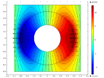
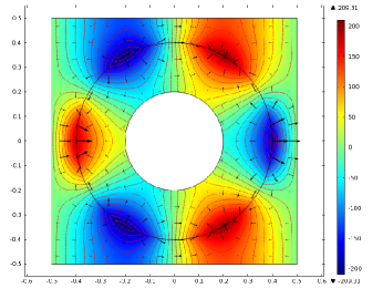
Figure 4: (a) the solution corresponding to the eigenvalue $\lambda=3.5080\times 10^{-1}$; (b) the solution corresponding to the eigenvalue $\lambda=1.5379\times 10^{-2}$.

6 Numerical calculation of the dispersion relation and comparison with power series

In this section we verify that the leading order dispersion relation expressed in terms of effective properties is a good predictor of the dispersive behavior of the metamaterial for periods with finite size $d>0$. The usefulness of the effective properties for predicting metamaterial behavior away from the homogenization limit can be explicitly seen from power series formula for the dispersion relation. To proceed we fix $d=c/\omega_{p}$ and the dimensionless ratio $\rho=d/\sqrt{\epsilon_{r}}$. With this choice of variables the frequency dependent effective magnetic permeability $\mu_{eff}$ and effective dielectric permittivity $\epsilon_{eff}$ are written as

$$\mu_{eff}(\omega_{0}/\omega_{p})=\int_{Y}\psi_{0}=\theta_{H}+\theta_{P}+\sum_{n=1}^{\infty}\frac{\mu_{n}<\phi_{n}>^{2}_{R}}{\rho^{-2}\left(\mu_{n}\rho^{2}-(\frac{\omega_{0}}{\omega_{p}})^{2}\right)}$$ (6.1)

and

$$\epsilon^{-1}_{eff}(\omega_{0}/\omega_{p})\hat{\kappa}\cdot\hat{\kappa} = \theta_{H}+\frac{(\frac{\omega_{0}}{\omega_{p}})^{2}}{(\frac{\omega_{0}}{\omega_{p}})^{2}-1}\theta_{P}$$

$$-\sum_{-\frac{1}{2}<\lambda_{h}<\frac{1}{2}}\left(\frac{\left((\frac{\omega_{0}}{\omega_{p}})^{2}-1\right)^{2}|\alpha_{\lambda_{h}}^{(1)}|^{2}+2\left((\frac{\omega_{0}}{\omega_{p}})^{2}-1\right)\alpha_{\lambda_{h}}^{(1)}\alpha_{\lambda_{h}}^{(2)}+|\alpha_{\lambda_{h}}^{(2)}|^{2}}{\left((\frac{\omega_{0}}{\omega_{p}})^{2}-(\lambda_{h}+\frac{1}{2})\right)\left((\frac{\omega_{0}}{\omega_{p}})^{2}-1\right)}\right).$$

In these variables the leading order dispersion relation is given by

$$(dk)^{2}=(\frac{\omega_{0}}{\omega_{p}})^{2}n_{eff}^{2},$$ (6.3)

where the effective index of diffraction $n_{eff}^{2}$ depends upon the direction of propagation $\hat{\kappa}$ and normalized frequency $\frac{\omega_{0}}{\omega_{p}}$ and is written

$$n_{eff}^{2}=\mu_{eff}(\frac{\omega_{0}}{\omega_{p}})/(\epsilon_{eff}^{-1}(\frac{\omega_{0}}{\omega_{p}})\hat{\kappa}\cdot\hat{\kappa}).$$ (6.4)

The dispersion relation for the metamaterial crystal in the new variables is given by

$$\left(\frac{\omega}{\omega_{p}}\right)^{2}=\left(\frac{\omega_{0}}{\omega_{p}}\right)^{2}+\sum_{l=1}^{\infty}(dk)^{l}\left(\frac{\omega_{l}}{\omega_{p}}\right)^{2},$$ (6.5)

for

$$\{-2\pi\leq dk\hat{\kappa}_{1}\leq 2\pi,-2\pi\leq dk\hat{\kappa}_{2}\leq 2\pi\}.$$ (6.6)

It is clear from (6.5) that the roots $\frac{\omega_{0}}{\omega_{p}}$ of the effective dispersion relation (6.3) determines the leading order dispersive behavior for periods of finite size. We point out that the notion of effective properties for metamaterials has proved to be an elegant concept for explaining experimental results. Here it is seen that the power series (6.5) exhibits the precise way in which effective properties influence leading order behavior for period cells of size $d>0$.

To verify that the leading order dispersion relation is a good predictor of the dispersive behavior of the metamaterial, we numerically compute the solutions $(\omega/\omega_{p})^{2}$ and $u^{d}$ of the nonlinear eigenvalue problem given by equation (2.6). These computations are carried out for different wave numbers $k$ with propagation along the direction $(1,0)$. The simulations are carried out using COMSOL software. Here we are interested in the range $\omega/\omega_{p}<1$ for which the plasmonic material has a negative permittivity, $\epsilon_{P}<0$. Two examples are considered: the first example is the case of $a=0.2d,b=0.4d$ and $\epsilon_{R}=\epsilon_{r}/d^{2}=285$ and the second example is for $a=0.15d,b=0.4d$ and $\epsilon_{R}=285$. Figure 5 (a)(b) (Figure6 (a)(b)) are the graphs of the effective properties $\epsilon^{-1}_{eff}(\frac{\omega_{0}}{\omega_{p}})\hat{\kappa}\cdot\hat{\kappa}$ and $\mu_{eff}(\frac{\omega_{0}}{\omega_{p}})$ respectively. Figure 5 (c) (Figure 6 (c)) compares the prediction given by the leading order dispersion relations $dk=\sqrt{n_{eff}^{2}}\frac{\omega_{0}}{\omega_{p}}$ (solid lines) with the numerical approximation of the dispersion relation given by black dots. Although the length scale of the microstructure is not infinitesimally small compared to the radiation wavelength, the numerically calculated points (black dots) fall near the solid lines predicted by the leading order dispersion relation. Notice that the magenta area is the prediction of the band of double negative leading order effective properties while the green area is for the double positive band. Both graphs show that the leading order dispersion relation given by the power series can well predict the Bloch wave modes in the actual crystal up to about $20\%$ smaller than the wavelength.

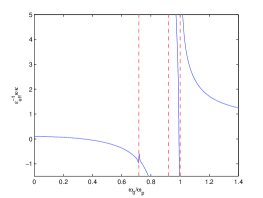
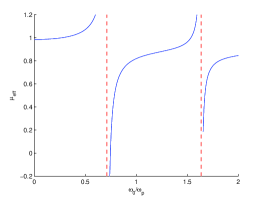
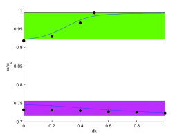
Figure 5: the case of $a=0.2d,b=0.4d$ and $\epsilon_{R}=285$. Notice that the vertical dash lines are the asymptotes.

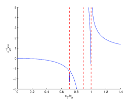
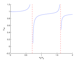
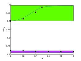
Figure 6: the case of $a=0.15d,b=0.4d$ and $\epsilon_{R}=285$. Notice that the vertical dash lines are the asymptotes.

The simulations show that the frequency range spanned by the double negative propagation bands increases as the thickness of the plasmonic coating decreases.

7 Acknowledgments

This research is supported by NSF grant DMS-0807265 and AFOSR grant FA9550-05-0008.

References

• [1] Alu, A. & Engheta, N. 2008 Dynamical theory of artifical optical magnetism produced by rings of plasmonic nanoparticles. Phys. Rev. B 78, 085112.
• [2] Alu, A. 2011 First principles homogenization theory for periodic metamaterial arrays. Phys Rev. B 84, 075153.
• [3] Bohren, C.F. & Huffman, D.H. 2004 Absorption and Scattering of Light by Small Particles, Wiley.
• [4] BouchittΓ© G. & Bourel, C. 2010 Homogenization of finite metallic fibers and 3D-effective permittivity tensor. Commun. Comput. Phys. To appear.
• [5] BouchittΓ©, G. & Schweizer, B. 2010 Homogenization of Maxwell’s equations in a split ring geometry. SIAM Multi. Model. Simu. 8, 717–750.
• [6] BouchittΓ©, G. & Felbacq, D. 2005 Negative refraction in periodic and random photonic crystals. New J. Phys. 7, 159.
• [7] BouchittΓ©, G. & Felbacq, D. 2004 Homogenization near resonances and artificial magnetism from dielectrics. C. R. Acad. Sci. Paris I 339, 377–382
• [8] Chen, Y. & Lipton, R. 2012 Resonance and double negative behavior in metamaterials. arXiv:1111.3586v2 [math.AP].
• [9] Chen, Y. & Lipton, R. 2010 Tunable double negative band structure from non-magnetic coated rods. New J. Phys. 12, 083010.
• [10] Chern, R. L. & Felbacq, D. 2009 Artificial magnetism and anticrossing interaction in photonic crystals and split-ring structures . Phys. Rev. B 79, 075118.
• [11] Dolling, G., Enrich, C., Wegener, M., Soukoulis, C. M. & Linden, S. 2006 Low-loss negative-index metamaterial at telecommunication wavelengths. Opt. Lett. 31, 1800–1802.
• [12] Felbacq, D. & Bouchitte, G. 2005 Homogenization of wire mesh photonic crystals embdedded in a medium with a negative permeability. Phys. Rev. Lett. 94), 183902.
• [13] Fortes, S. P., Lipton, R. P. & Shipman, S. P. 2009 Sub-wavelength plasmonic crystals: dispersion relations and effective properties. Proc. R. Soc. A 466 , 1993–2020. (doi: 10.1098/rspa.2009.0542)
• [14] Fortes, S. P., Lipton, R. P. & Shipman, S. P. 2011 Convergent power series for fields in positive or negative high-contrast periodic media. Comm. Partial Differential Equations 36, 1016–1043.
• [15] Huangfu, J., Ran, L., Chen, H., Zhang, X., Chen, K., Grzegorczyk, T. M. & Kong, J. A. 2004 Experimental confirmation of negative refractive index of a metamaterial composed of $\Omega$-like metallic patterns. Appl. Phys. Lett. 84, 1537.
• [16] Huang, K., C., Povinelli, M., L. & Joannopoulos, J. D. 2004 Negative effective permeability in polaritonic photonic crystals. Appl. Phys.Lett. 85, 543.
• [17] Kohn, R. & Shipman, S. 2008 Magnetism and homogenization of micro- resonators. SIAM Multi. Model. Simu. 7, 62–92.
• [18] McPhedran, R.C., Nicorovici, N.A., Botten, L.C. & Movchan, A.B. 2001 Advances in the Rayleigh multipole method for problems in photonics and phononics. IUTAM Symposium on Mechanical and Electromagnetic Waves in Structured Media (ed. R.C. McPhedran et al), pp. 15–28, Kluwer Academic Publishers.
• [19] Milton, G. W. 2010 Realizability of metamaterials with prescribed electric permittivity and magnetic permeability tensors. New J. Phys. 12, 033035.
• [20] Nicorovici, N.A., McPhedran, R.C. & Milton, G.W. 1993 Transport properties of a 3 phase composite material: the square array of coated cylinders. Proc. R. Soc. A 422, 599–620.
• [21] Pendry, J., Holden, A., Robbins, D. & Stewart, W. 1999 Magnetisim from conductors and enhanced nonlinear phenomena. IEEE Trans. Microwave Theory Tech. 47, 2075–2084.
• [22] Pendry, J., Holden, A., Robbins, D. & Stewart, W. 1998 Low frequency plasmons in thin-wire structures. J. Phys.: Condens. Matter 10, 4785–4809.
• [23] Peng, L., Ran, L., Chen, H. , Zhang, H., Kong, L. A. & Grzegorczyk, T. M. 2007 Experimental observation of left-handed behavior in an array of standard dielectric resonators. Phys. Rev. Lett. 98, 157403.
• [24] Perrins. W.T., McKenzie, D.R. & McPhedran, R.C. 1979 Transport properties of regular arrays of cylinders. Pro. R. Soc. A 369 207–225.
• [25] Service, R. F. 2010 Next Wave of metamaterials hopes to fuel the revolution. Sci. 327, 138–139.
• [26] Shalaev, V. 2007 Optical negative-index metamaterials. Nature Photonics 1, 41-48.
• [27] Shalaev, V. M., Cai, W., Chettiar,U. K., Yuan, H. K., Sarychev, A. K., Drachev, V. P. & Kildishev, A. V. 2005 Negative index of refraction in optical metamaterials. Opt. Lett. 30, 3356–3358.
• [28] Shelby, R.A., Smith D.R. & Schultz, S. 2001 Experimental verification of a negative index of refraction. Sci. 292, 77–79.
• [29] Shipman, S. 2010 Power series for waves in micro-resonator arrays. In Proceedings of the 13th International Conference on Mathematical Methods in Electrodynamic Theory, Kyiv, Ukraine: IEEE.
• [30] Shvets, G. & Urzhumov, Y.: Engineering the electromagnetic prop- erties of periodic nanostructures using electrostatic resonances. Phys. Rev. Lett. 93, 243902-1-4.
• [31] Smith D.R. & Pendry J.B. 2006 Homogenization of metamaterials by field averaging. J. Opt. Soc. Am. B. 23, 391–403.
• [32] Smith, D., Padilla, W., Vier, D., Nemat-Nasser, S. & Schultz, S. 2000 Composite medium with simultaneously negative permeability and permittivity. Phys. Rev. Lett. 84, 4184–4187.
• [33] Strutt, J.W. 1892 On the influence of obstacles arranged in rectangular order upon the properties of a medium. Phil. Mag. 34, 481–502.
• [34] Veselago, V., G. 1968 The electrodynamics of substances with simultaneously negative values of $\epsilon$ and $\mu$. Sov. Phys. Usp. 10, 509.
• [35] Vynck, K., Felbacq, D., Centeno, E., Cabuz, A. I., Cassagne, D. & Guizal, B. 2009 All-dielectric rod-type metamaterials at optical frequencies. Phys. Rev. Lett. 102, 133901.
• [36] Wheeler, M. S., Aitchison, J. S. & Mojahedi, M. 2006 Coated non-magnetic spheres with a negative index of refraction at infrared frequencies . Phys. Rev. B 73, 045105.
• [37] Yannopapas, V. 2007 Negative refractive index in the near-UV from Au-coated CuCl nanoparticle superlattices. Phys. Stat. Sol. (RRL) 1, 208–210.
• [38] Yannopapas, V. 2007 Artificial magnetism and negative refractive index in three-dimensional metamaterials of spherical particles at near-infrared and visible frequencies. Appl. Phys. A 87, 259–264.
• [39] Zhang, F., Potet, S., Carbonell, J., Lheurette, E., Vanbesien, O., Zhao, X. & Lippens, D. 2008 Negative-zero-positive refractive index in a prism-like omega-type metamaterial . IEEE Trans. Microw. Theory Tech. 56, 2566.
• [40] Zhang, S., Fan, W., Minhas, B. K., Frauenglass, A., Malloy, K. J. & Brueck, S. R. J. 2005 Midinfrared resonant magnetic nanostructures exhibiting a negative permeability. Phys. Rev. Lett. 94, 037402.
• [41] Zhou, X. & Zhao, X. P. 2007 Resonant condition of unitary dendritic structure with overlapping negative permittivity and permeability. Appl. Phys. Lett. 91, 181908.