Rebound-through transition of bright-bright solitons collision in two species condensates with repulsive interspecies interactions

Abstract

Abstract: We study the dynamical properties of bright-bright solitons in two species Bose-Einstein condensates with the repulsive interspecies interactions under the external harmonic potentials by using a variational approach combined with numerical simulation. It is found that the interactions between bright-bright solitons vary from repulsive to attractive interactions with the increasing of their separating distances. And the bright-bright solitons can be localized at equilibrium positions, different from the periodic oscillation of bright soliton in the single species condensates. Especially, a through-collision is newly observed from the bright-bright solitons collisions with the increasing of the initial velocity. The collisional type of bright-bright solitons, either rebound - or through -collision, depends on the modulation of the initial conditions. These results will be helpful for the experimental manipulating such solitons. PACS (2008): 05.45.Yv, 03.75.Lm, 03.75.Mn Keywords: Bright-bright solitons ${\bullet}$ two species BECs ${\bullet}$ collisions

1. Introduction

Recently, matter wave soliton pairs of dark-dark solitons and dark-bright solitons have been experimentally observed in two species Bose-Einstein condensates (BECs) [1-7]. In the experiment, an external magnetic gradient is applied to make the two species BECs undergo phase separation [1, 2]. In the phase separation regime, the bright soliton in one species can be stably trapped inside a density dip of the dark soliton in the other species [3], while it can not occur in the single species BECs. This means that the lifetime of bright soliton in two-species BECs [3] is longer than that of one in the single species BECs [8, 9]. This long-lived bright solitons may open possibilities for future applications in coherent atomic optics, atom interferometry, and atom transport.

The possibility of creating soliton pairs in two species BECs has stimulated considerable theoretical interest in their existence conditions, stability, interactions, collisions, and so on [10-34]. Based on the mean-field theory, the solitons properties in the two species BECs are usually described by the coupled Gross-Pitaevskii (GP) equation, which is similar to the coupled nonlinear Schr$\ddot{\textrm{o}}$dinger equation (NLSE) used in nonlinear optics. Some literatures showed that in the absence of the external potentials, the interactions between the bright-bright solitons (BBSs) are mainly determined by the interspecies interactions of two species BECs [10-12]. In this case, for the attractive (repulsive) interspecies interaction, there is an attractive (repulsive) potential between the BBSs, and thus they exhibited always attraction [10, 11] (repelsion [12]) each other. Taking into account the external harmonic potential, we here explore the dynamical properties of BBSs in two species BECs. It is found that the interactions between BBSs vary from repulsive to attractive interactions with the increasing of their separating distances, even for repulsive interspecies interactions. And the BBSs can be localized at the equilibrium position, different from the periodic oscillation of bright soliton in the single species condensates.

In addition, the interspecies interactions of two species BECs have important effect on the collisional properties of BBSs [13-17]. For the attractive interactions, a through-collision (TC) occurs between the BBSs [13, 14]. Such solitons pass through each other at the collision point, and the TC is independent of the initial conditions, such as the separating distances and velocities [14]. For the repulsive interspecies interactions, there exists a regime of elastic particle collisions [15], where there occurs a rebound-collision (RC) with a momentum exchange between the BBSs. It is worthwhile pointing out that, in nonlinear optics, the collisional type of BBSs can be controlled by their initial velocities [17].

To our knowledge, there is little report on the effect of the initial velocity and separating distance on the collisional properties of BBSs in two species BECs with the repulsive interspecies interactions. Therefore, considering the repulsive interspecies interactions and external harmonic potentials, we explore the collisions between BBSs with different initial velocities and separating distance. It is found that a TC is newly observed from the BBSs collisions with the increasing of the initial velocity. And the collisional type of BBSs, either TC or RC, depends on the modulation of the initial conditions.

2. Model

We consider that the two species BECs are trapped in the harmonic potentials [30-34]$\emph{V}^{(\emph{i})}_{\emph{ext}}(\emph{X},\emph{Y},\emph{Z})=\emph{M}_{\emph{i}}[\omega^{2}_{\bot(\emph{i})}(\emph{Y}^{2}+\emph{Z}^{2})+\omega^{2}_{\emph{i}}\emph{X}^{2}]/2$. Here, $\omega_{\bot(\emph{i})}$ and $\omega_{\emph{i}}$ are the radial and transverse trapping frequencies with $\emph{i}=1,2$, and $\emph{M}_{\emph{i}}$ is the atomic mass of the $\emph{i}^{th}$ species. If $\omega_{\bot(\emph{i})}\gg\omega_{\emph{i}}$ , it is reasonable to reduce the GP equation to a coupled one-dimensional NLSE

$$i\hbar\frac{\partial\Psi_{1}(X,T)}{\partial T}=[-\frac{\hbar^{2}}{2M_{1}}\frac{\partial^{2}}{\partial X^{2}}+2\hbar\omega_{\bot(1)}a_{1}N_{1}|\Psi_{1}|^{2}$$

$$+\frac{\hbar\omega_{\bot(1)}a_{12}M_{1}N_{1}}{M}|\Psi_{2}|^{2}+\frac{M_{1}\omega^{2}_{1}X^{2}}{2}]\Psi_{1},$$ (1)

$$i\hbar\frac{\partial\Psi_{2}(X,T)}{\partial T}=[-\frac{\hbar^{2}}{2M_{2}}\frac{\partial^{2}}{\partial X^{2}}+\frac{2\hbar\omega_{\bot(1)}M_{1}a_{2}N_{2}}{M_{2}}|\Psi_{2}|^{2}$$

$$+\frac{\hbar\omega_{\bot(1)}M_{1}a_{12}N_{2}}{M}|\Psi_{1}|^{2}+\frac{M_{2}\omega^{2}_{2}X^{2}}{2}]\Psi_{2},$$ (2)

where $N_{i}(\emph{i}=1,2)$ is the atoms number of the $i^{th}$ species; $a_{i}$ and $a_{12}$ are the intraspecies and interspecies scattering length (SL), respectively; and $1/M=1/M_{1}+1/M_{2}$. Subsequently, we introduce some dimensionless variables $X=a_{\bot}x$, $T=2t/\omega_{\bot(1)}$, and $\psi_{i}=a_{\bot}\Psi_{i}$, with $a_{\bot}=\sqrt{\hbar/M_{1}\omega_{\bot(1)}}$, so that Eqs. (1) and (2) are reduced into

$$[i\frac{\partial}{\partial t}+\frac{\partial^{2}}{\partial x^{2}}+g_{11}|\psi_{1}|^{2}-g_{12}|\psi_{2}|^{2}-\frac{\omega^{2}_{1}x^{2}}{\omega^{2}_{\bot(1)}}]\psi_{1}=0,$$ (3)

$$[i\frac{\partial}{\partial t}+\frac{\partial^{2}}{\partial x^{2}}+\varepsilon g_{22}|\psi_{2}|^{2}-\varepsilon g_{21}|\psi_{1}|^{2}-\frac{\omega^{2}_{2}x^{2}}{\varepsilon\omega^{2}_{\bot(1)}}]\psi_{2}=0,$$ (4)

where $\varepsilon=M_{1}/M_{2}$, $g_{ii}=-4a_{i}N_{i}/a_{\bot}$, $g_{12}=2a_{12}M_{1}N_{1}/(Ma_{\bot})$, and $g_{21}=2a_{12}M_{2}N_{2}/(Ma_{\bot})$. We here consider the two species BECs composed of ⁷Li and ³⁹K atoms which is accessible for experiments, and the species one (two) is ⁷Li (³⁹K) condensate. Based on the currently experimental conditions, the radial trapping frequencies are chosen as $\omega_{\bot(1)}=\omega_{\bot(2)}=2\pi\times 100$ Hz, so that the time and space units correspond to 6.4 ms and 5.4 $\mu m$ in reality, respectively. We also choose the atom numbers $N_{1}=N_{2}=2000$, the intraspecies SLs $a_{1}=-25$ $a_{B}$ and $a_{2}=-139$ $a_{B}$, respectively, and interspecies SL $a_{12}=-42.4$ $a_{B}$. Here, $a_{B}$ is Bohr radius.

3. Variational approach

When the interspecies interactions were repulsive, the BBSs exhibited repelsive each other [12]. It means that there is a repulsive potential between the BBSs. In order to obtain this effective potential, we solve Eqs. (3) and (4) by using a variational approach [10]. We here propose that $\omega_{1}=\omega_{2}=0$, in this case, the ansatz solitons solutions of Eqs. (3) and (4) are chosen as

$$\psi_{j}(x,t)=\frac{a(t)\exp[i\eta_{j}(t)(x-x_{j}(t))+i\mu_{j}(t)]}{\cosh[\kappa a(t)(x-x_{j}(t))]},$$ (5)

where $\kappa$ is constant; $a$, $x_{j}$, $\eta_{j}$, and $\mu_{j}$ are the functions of time $t$ with $j=1,2$. So, the Lagrangian density $\Gamma$ can be given by

$$\Gamma=\sum^{2}_{j=1}[\frac{i}{2}(\bar{\psi_{j}}\frac{\partial\psi_{j}}{\partial t}-\psi_{j}\frac{\partial\bar{\psi_{j}}}{\partial t})-|\frac{\partial\psi_{j}}{\partial x}|^{2}$$

$$+\frac{g_{jj}|\psi|^{4}}{2}]-g_{12}|\psi_{1}|^{2}|\psi_{2}|^{2}.$$ (6)

Here, the overbar denotes the complex conjugate. Substituting Eq. (5) into Eq. (6) and then integrating the result over $x$ from $-\infty$ to $\infty$, we obtain the Lagrangian

$$L=\sum^{2}_{j=1}[2\frac{a}{\kappa}(\eta_{j}\frac{\partial x_{j}}{\partial t}-\eta^{2}_{j}-\frac{\partial\mu_{j}}{\partial t})+\frac{2a^{3}(g_{jj}-\kappa^{2})}{3\kappa}]$$

$$-\frac{4g_{12}a^{3}A(x_{2}-x_{1})}{\kappa},$$ (7)

where

$$A=\frac{{\kappa a(x_{2}-x_{1})\cosh[\kappa a(x_{2}-x_{1})]-\sinh[\kappa a(x_{2}-x_{1})]}}{\sinh^{3}[\kappa a(x_{2}-x_{1})]}.$$ (8)

The action is defined as $I=\int^{t2}_{t1}Ldt$ . We can get a set of equations for the ansatz parameters from the least-action principle $\delta I=0$ . They are given by

$$\delta I/\delta\mu_{j}=0\rightarrow a=\textrm{constant},$$ (9)

$$\delta I/\delta\eta_{j}=0\rightarrow\partial x_{j}/\partial t=2\eta_{j},$$ (10)

$$\delta I/\delta x_{j}=0\rightarrow\partial\eta_{j}/\partial t=-2g_{12}a^{2}\partial A/\partial x_{j},$$ (11)

$$\delta I/\delta a=0\rightarrow\partial\mu_{j}/\partial t=\eta_{j}\partial x_{j}/\partial t-\eta^{2}_{j}$$

$$+2a^{2}(g_{jj}-\kappa^{2})-4g_{12}a^{2}A/3,$$ (12)

where $j=1,2$. From the Eqs. (10) and (11), we get

$$\partial_{t}(a^{2}\frac{\partial x_{1}}{\partial t}+a^{2}\frac{\partial x_{2}}{\partial t})=-4g_{12}a^{4}(\partial_{x_{1}}+\partial_{x_{2}})A=0,$$ (13)

and Newton’s motion equation

$$a^{2}\frac{\partial^{2}x_{j}}{\partial t^{2}}=-4g_{12}a^{4}\frac{\partial A}{\partial x_{j}},$$ (14)

where $j=1,2$. Accordingly, we obtain

$$a^{2}\frac{\partial x_{1}}{\partial t}+a^{2}\frac{\partial x_{2}}{\partial t}=P,$$ (15)

$$\frac{1}{2}a^{2}\frac{\partial x^{2}_{1}}{\partial t}+\frac{1}{2}a^{2}\frac{\partial x^{2}_{2}}{\partial t}+4g_{12}a^{4}A=E,$$ (16)

where $P$ and $E$ are integral constants. If we take $a^{2}$ as the mass of the soliton, equations (15) and (16) represent the conservation of momentum and energy of the solitons, respectively. In Eq. (16), we can define the effective potential $V_{eff}(q)$ [10]

$$V_{eff}(q)=4g_{12}a^{4}[\frac{{\kappa aq\cosh(\kappa aq)-\sinh(\kappa aq)}}{\sinh^{3}(\kappa aq)}].$$ (17)

Here $q=x_{2}-x_{1}$ represents the separating distances of two solitons. For a better understanding this effective potential between the BBSs, we plot the effective potential varying with the separating distance in Fig. 1. One can see that with the increasing value of separating distance q, the effective potential $V_{eff}(q)$ decreases. And when $q$ increases a defined value, the effective potential vanishes. This manifests that the force between the BBSs is a short-range force.

Figure 1: Variations of the effective potential with the separating distance. The parameters used are $a=1.0$, $g_{12}=2.0$, and $\kappa=0.882$.

4. The interaction forces between two solitons

To obtain interaction forces between the BBSs, we here numerically simulate the Eq. (2) by the Crank-Nicolson method [34]. The initial conditions are chosen as [15]

$$\psi_{j}(x,0)=\frac{b_{j}\exp(2ic_{j}x)}{\cosh[b_{j}(x-x_{j})]},$$ (18)

where $b_{j}$, $x_{j}$, and $c_{j}$ are constant with $j=1,2$. To get the range of the interspecies interaction force, we first consider that the transverse trapping frequencies $\omega_{1}=\omega_{2}=0$. The corresponding bright solitons positions varying with the time $t$ are shown in Fig. 2. One can see from Fig. 2(a) that at the initial time, the bright soliton of species one is at $x_{1}=3.00$, and the bright soliton of (the other) species two is at $x_{2}=-3.00$. The initial velocities of solitons are set as $c_{1}=c_{2}=0$. With the time going on, the bright soliton of species one moves along the positive direction of x-axis, and the other one moves along the negative direction of x-axis. This indicates that there exists a repulsive force between the bright solitons. While the initial positions are displaced at $x_{1}=-x_{2}=4.20$ and the initial velocities are still set as $c_{1}=c_{2}=0$ [see Fig. 2(b)], the position of each soliton keeps unchanged with the time going on. It means that the repulsive force between two solitons vanishes. In this case, we can obtain that the range of this repulsive force is the separating distance $q\leq 8.40$. In addition, from the inset of Fig. 1, it makes sure that when the separating distance $q=8.40$, the $V_{eff}(q)\approx 10^{-4}\approx 0$. So the numerical result is in good agreement with the result of the variational approach.

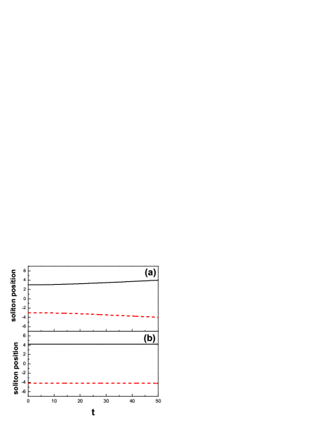
Figure 2: (Color online) Evolvement of the solitons positions in two species BECs with the repulsive interspecies interactions. The initial positions of two solitons are (a) $x_{1}=2.00$, $x_{2}=-2.00$, and (b) $x_{1}=4.20$, $x_{2}=-4.20$, respectively. The other parameters used are $b_{1}=1.0$, $b_{2}=1.0$, $c_{1}=0$, $c_{2}=0$, $g_{11}=2.0$, $g_{22}=2.0$, $g_{12}=2.0$, $\omega_{1}=0$, and $\omega_{2}=0$. Solid and dash lines correspond to the species one and two, respectively.

We then choose the transverse trapping frequencies $\omega_{1}=1.4\pi$ Hz and $\omega_{2}=0.6\pi$ Hz to explore the interaction forces between the BBSs. Figure 3 shows the corresponding solitons positions varying with the time. In this case, the initial velocities of two solitons are still set as $c_{1}=c_{2}=0$. One can see from Fig. 3(a) that at the initial time, the bright soliton of species one is at $x_{1}=2.00$, and the bright soliton of species two is at $x_{2}=-2.00$. With the time going on, the bright soliton of species one moves along the positive direction of x-axis, and the other one moves along the negative direction of x-axis. This indicates that the interaction between two soliton is repulsive. While the initial positions of two solitons are displaced at $x_{1}=-x_{2}=4.00$ [see Fig. 3(b)], it is interesting to see that the bright soliton of species one moves along the negative direction of x-axis, and the other one moves along the positive direction of x-axis. This indicates that the interaction between two solitons is attractive. We here can conclude that the interactions between the BBSs vary from repulsive to attractive with the increasing of the separating distance. In fact, when two solitons are trapped in the harmonic potentials, each soliton undergoes two forces which are from the external potentials and interspecies interactions. For convenience, we here defined $F_{1(i)}$ and $F_{2(i)}$ $(i=1,2)$ represent the forces coming from the external potentials and interspecies interactions, respectively. That is $F_{1(i)}=-dV_{trap}(x_{i})/dx_{i}=-2\omega^{2}_{x(1)}x_{i}/\omega^{2}_{\bot(1)}$ and $F_{2(i)}=-\partial V_{eff}(q)/\partial x_{i}$ with $i=1,2$. When the two bright solitons are at $x_{1}=2.00$ and $x_{2}=-2.00$, respectively, [such as in Fig. 3(a)], we have $F_{1(1)}=-F_{1(2)}\approx-0.00800$ and $F_{2(1)}=-F_{2(2)}\approx 0.13428$. Duo to that $|F_{2}|>|F_{1}|$, two solitons undergo repulsive interactions each other. While the two bright solitons are at $x_{1}=4.00$ and $x_{2}=-4.00$, respectively, [such as in Fig. 3(b)], there are $F_{1(1)}=-F_{1(2)}\approx-0.01600$ and $F_{2(1)}=-F_{2(2)}\approx 0.00030$, so that $|F_{2}|<|F_{1}|$ and thus two solitons attract each other. That is to say, the interactions between two solitons, either attractive or repulsive, depend on the difference between the absolute value of $F_{1}$ and $F_{2}$.

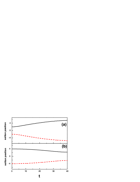
Figure 3: (Color online) Evolvement of the solitons positions in two species BECs with the repulsive interspecies interactions and external harmonic potentials. The initial positions of two solitons are (a) $x_{1}=2.00$, $x_{2}=-2.00$, and (b) $x_{1}=4.00$, $x_{2}=-4.00$, respectively. The parameters used are $\omega_{1}=1.4\pi$ Hz and $\omega_{2}=0.6\pi$ Hz. The other parameters used are the same as the figure 2. Solid and dash lines correspond to the species one and two, respectively.

In addition, if the two bright solitons newly displace at $x_{1}=2.84$ and $x_{2}=-2.84$, respectively, there are $F_{1(1)}=-F_{1(2)}\approx-0.01136$ and $F_{2(1)}=-F_{2(2)}\approx 0.01135$, so that $|F_{2}|\approx|F_{1}|$. In this case, the propagating characteristics of two bright solitons are shown in Fig. 4. One sees that the width, amplitude, and position of each soliton keep unchanged with time. Obviously, they are localized solitons, different from the periodic oscillation of bright soliton in the single species BECs [35,36]. Thanks to the two balance forces, the lifetime of the bright solitons in two-species BECs at the equilibrium positions should be longer than that of one in the single BECs. These stable bright solitons may open possibilities for future applications in coherent atomic optics.

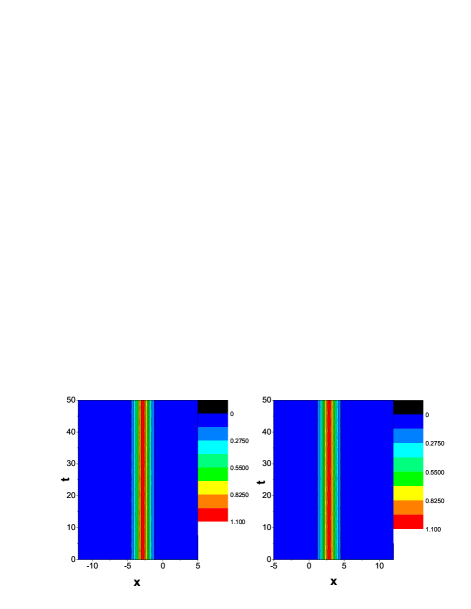
Figure 4: (Color online) The propagating characteristics of BBSs in two species BECs with the repulsive interspecies interactions and external harmonic potentials. The parameters used are $x_{1}=2.84$, $x_{2}=-2.84$, $\omega_{1}=1.4\pi$ Hz and $\omega_{2}=0.6\pi$ Hz. The other parameters are the same as the figure 2. The right and left plots represent the density of the species one and two, respectively.

From discussed above, we conclude that the interaction forces between BBSs of two species BECs trapped in the harmonic potentials exhibit either attraction or repulsion, which is controlled by their initial separating distance. And the BBSs can be localized at equilibrium positions of two equal forces.

5. The collision properties of BBSs

In order to explore the effect of initial velocity on the collision properties of BBSs, we here consider the two bright solitons are at the equilibrium positions (which are at $x_{1}=2.84$ and $x_{2}=-2.84$, respectively). Figure 5 shows the soliton positions as a function of the time with the different initial velocity. When the initial velocities of two solitons are $c_{1}=0.1$ and $c_{2}=-0.1$ [as shown in Fig. 5(a)], respectively, the two solitons move towards each other and take place a collision at $t\approx 5$. They do not pass through each other at the collision point, so, this collision belongs to RC. This phenomenon is similar with the report in Ref. [15]. While the initial velocities of two solitons are increased to $c_{1}=0.7$ and $c_{2}=-0.7$ [see Fig. 5(b)], respectively. Interestingly, it is observed that the two bright solitons pass through each other at the time $t\approx 1.2$. This collision is TC. The followed TC behavior can be observed at $t\approx 10$ and $t\approx 18.5$. This shows that the collision type of BBSs exhibits a transition from RC to TC.

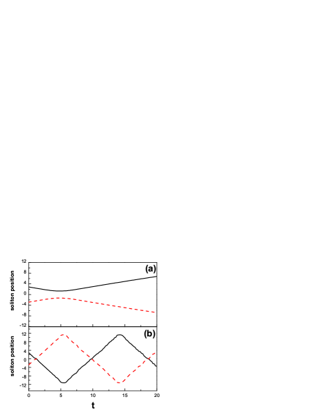
Figure 5: (Color online) Evolvement of the solitons positions with the different initial velocities. The initial velocities of two solitons are (a) $c_{1}=0.1$, $c_{2}=-0.1$, (b) $c_{1}=0.7$, $c_{2}=-0.7$, respectively. The parameters used are $x_{1}=2.84$, $x_{2}=2.84$, $\omega_{1}=1.4\pi$ Hz and $\omega_{2}=0.6\pi$ Hz. The other parameters are the same as the figure 2. Solid and dash lines correspond to the species one and two, respectively.

Subsequently, in order to get the effect of initial separating distance on the collision properties of BBSs, we propose that the initial velocities of two solitons are $c_{1}=0.8$ and $c_{2}=-0.8$, respectively. The corresponding collisional behaviors of BBSs with different initial separating distance are plotted in Fig. 6. When two solitons are at $x_{1}=2.00$ and $x_{2}=-2.00$, respectively [see Fig. 6(a)], one can see that the collisions between two solitons are all TC. While the initial positions of two solitons are newly displaced at $x_{1}=5.20$ and $x_{2}=-5.20$ [as shown in Fig. 6(b)], respectively, it is interesting to observe that the collisions between two solitons are all RC.

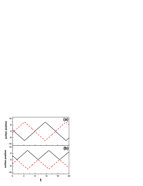
Figure 6: (Color online) Evolvement of the solitons positions in two species BECs with the different initial separating distance. The initial positions of two solitons are (a) $x_{1}=2.00$, $x_{2}=-2.00$, (b) $x_{1}=5.20$, $x_{2}=-5.20$, respectively. The parameters used are $b_{1}=2.0$, $b_{2}=2.0$, $c_{1}=0.8$, $c_{2}=-0.8$, $\omega_{1}=1.4\pi$ Hz and $\omega_{2}=0.6\pi$ Hz. The other parameters are the same as the figure 2. Solid and dash lines correspond to the species one and two, respectively.

We here can conclude that the collisional type of BBSs, either TC or RC, depends on their initial velocities and separating distance. These results will be helpful for the experimental manipulating such BBSs.

6. Conclusion

In summary, we investigate the dynamical properties of BBSs in two species BECs with the repulsive interspecies interaction under the external harmonic potentials. Using the variational approach, we obtain the effective repulsive potential inducing by the interspecies interactions. By analyzing this effective potential, we find that the repulsive force between the BBSs is a short-range force. Then, we numerical simulate the dynamical properties of BBSs in the coupled one-dimensional NLSE by the Crank-Nicolson method. It is shown that the interactions between BBSs vary from repulsive to attractive interaction with the increasing of their separating distance. And the BBSs can be localized at equilibrium positions. These stable solitons may open possibilities for future applications in coherent atomic optics. Moreover, it is found that the TC is newly observed from the BBSs collisions with the increasing of their initial velocities. And the collisional type of BBSs, either TC or RC, depends on the modulation of the initial conditions.

References

References

- (1) C. Hamner, J.J. Chang, P. Engels, M.A. Hoefer, Phys. Rev. Lett. 106, 065302 (2011)
- (2) M.A. Hoefer, J.J. Chang, C. Hamner, P. Engels, Phys. Rev. A 84, 041605 (2011)
- (3) C. Becker, S. Stellmer, P. Soltan-Panahi, S. Drscher, M. Baumert, Eva-Maria Richter, Jochen Kronjger, K. Bongs, K. Sengstock, Nat. Phys. 4, 496 (2008)
- (4) G. Thalhammer, G. Barontini, L. DeSarlo, J. Catani, F. Minardi, M. Inguscio, Phys. Rev. Lett. 100, 210402 (2008)
- (5) Th. Best, S. Will, U. Schneider, L. Hackerm ller, D. van Oosten, I. Bloch, D.-S. L hmann, Phys. Rev. Lett. 102, 030408 (2009)
- (6) S.B. Papp, J.M. Pino, C.E. Wieman, Phys. Rev. Lett. 101, 040402 (2008)
- (7) G. Roati, M. Zaccanti, C. D’Errico, J. Catani, M. Modugno, A. Simoni, M. Inguscio, G. Modugno, Phys. Rev. Lett. 99, 010403 (2007)
- (8) K.E. Strecker, G.B. Partridge, A.G. Truscott, R.G. Hulet, Nature 417, 150 (2002)
- (9) L. Khaykovich, F. Schreck, G. Ferrari, T. Bourdel, J. Cubizolles, L.D. Carr, Y. castin, C. Salomon, Science 296, 1290 (2002)
- (10) H.Y. Yu, L.X. Pan, J.R. Yan, J.Q. Tang, J. Phys. B: At. Mol. Opt. Phys. 42, 0253019 (2009)
- (11) S.K. Adhikari, Phys. Lett. A 346, 179 (2005)
- (12) G. Csire, D. Schumayer, B. Apagyi, Phys. Rev. A 82, 063608 (2010)
- (13) X.F. Zhang, X.H. Hu, X.X. Liu, W.M. Liu, Phys. Rev. A 79, 033630 (2009)
- (14) L. Salasnich, B.A. Malomed, Phys. Rev. A 74, 053610 (2006)
- (15) D. Novoa, B.A. Malomed, H. Michinel, V.M. Prez-Garca, Phys. Rev. Lett. 101, 144101 (2008)
- (16) V. M. Prez-Garca, J. B. Beitia, Phys. Rev. A 72, 033620 (2005)
- (17) J.K. Yang, Y. Tan, Phys. Rev. Lett. 85, 3624 (2000)
- (18) X.X. Liu, H.Pu, B. Xiong, W.M. Liu, J.B. Gong, Phys. Rev. A 79, 013423 (2009)
- (19) D.S. Wang, X.H. Hu, W.M. Liu, Phys. Rev. A 82, 023612 (2010)
- (20) U. Shrestha, J. Javanainen, J. Ruostekoski, Phys. Rev. Lett. 103, 190401 (2009)
- (21) K.J.H. Law, P.G. Kevrekidis, L.S. Tuckerman, Phys. Rev. Lett. 105, 160405 (2010)
- (22) Th. Busch, J. R. Anglin, Phys. Rev. Lett. 87, 010401 (2001)
- (23) P. hberg, L. Santos, Phys. Rev. Lett. 86, 2918 (2001)
- (24) P. hberg, L. Santos, J. Phys. B: At. Mol. Opt. Phys. 34, 4271 (2001)
- (25) M. Vijayajayanthi, T. Kanna, M. Lakshmanan, Phys. Rev. A 77, 013820 (2008)
- (26) L. Li, B.A. Malomed, D. Mihalache, W.M. Liu, Phys. Rev. E 73, 066610 (2006)
- (27) L. Li, Z.D. Li, B.A. Malomed, D. Mihalache, W.M. Liu, Phys. Rev. A 72, 033611 (2005)
- (28) V.A. Brazhnyi, V.V. Konotop, Phys. Rev. E 72, 026616 (2005)
- (29) H.E. Nistazakis, D.J. Frantzeskakis, P.G. Kevrekidis, B.A. Malomed, R. Carretero-Gonz lez, Phys. Rev. A 77, 033612 (2008)
- (30) A.I. Yakimenko, Y.A. Zaliznyak, V.M. Lashkin, Phys. Rev. A 79, 043629 (2009)
- (31) S.K. Adhikari, Phys. Lett. A 346, 179 (2005)
- (32) V.M. Lashkin, E.A. Ostrovskaya, A.S. Desyatnikov, Y.S. Kivshar, Phys. Rev. A 80, 013615 (2009)
- (33) L.C. Zhao, S.L. He, Phys. Lett. A 375, 3017 (2011)
- (34) K. Kasamatsu, M. Tsubota, Phys. Rev. A 74, 013617 (2006)
- (35) U. Al Khawaja, H.T.C. Stoof, R.G. Hulet, K.E. Strecker, G.B. Partridge, Phys. Rev. Lett. 89, 200404 (2002)
- (36) P.K. Shukla, D.D. Tskhakaya, Phys. Scripta 107, 259 (2004)