Comparing Background Subtraction Algorithms and
Method of Car Counting

Abstract

In this paper, we compare various image background subtraction algorithms with the ground truth of cars counted. We have given a sample of thousand images, which are the snap shots of current traffic as records at various intersections and highways. We have also counted an approximate number of cars that are visible in these images. In order to ascertain the accuracy of algorithms to be used for the processing of million images, we compare them on many metrics that includes (i) Scalability (ii) Accuracy (iii) Processing time.

1 Introduction

There are thousands, if not millions, of outdoor cameras currently connected to the Internet, which are placed by governments, companies, conservation societies, national parks, universities, and private citizens. We view the connected global network of webcams as a highly versatile platform, enabling an untapped potential to monitor global trends, or changes in the flow of the city, and providing large-scale data to realistically model vehicular, or even human mobility. We developed a crawler that collects vehicular mobility traces from these online webcams. A majority of these webcams are deployed by city’s Department of Transportations (DoT). These web cameras are installed on traffic signal poles facing towards the roads of some prominent intersections throughout city and highways. At regular interval of time, they capture still pictures of on-going road traffic and send them in the form of feeds to the DoTs media server. For the purpose of this study, we made agreements with DoTs of 10 cities with large coverage to collect these vehicular imagery data for several months. We cover cities in North America, Europe, Asia, and Australia.

City	# of Cameras	Duration	Records
Bangalore	160	30/Nov/10 - 01/Mar/11	2.8 million
Beaufort	70	30/Nov/10 - 01/Mar/11	24.2 million
Connecticut	120	21/Nov/10- 20/Jan/11	7.2 million
Georgia	777	30/Nov/10 - 02/Feb/11	32 million
London	182	11/Oct/10 - 22/Nov/10	1 million
London(BBC)	723	30/Nov/10 - 01/Mar/11	20 million
New york	160	20/Oct/10 - 13/Jan/11	26 million
Seattle	121	30/Nov/10 - 01/Mar/11	8.2 million
Sydney	67	11/Oct/10 - 05/Dec/10	2.0 million
Toronto	89	21/Nov/10 - 20/Jan/11	1.8 million
Washington	240	30/Nov/10 - 01/Mar/11	5 million
Total	2709	-	125.2 million

Table 1: Global Webcam Datasets

 

(a) London

(b) Sydney

Figure 1: The red dots show the location of cameras in London and Sydney.

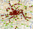
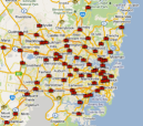
Since, these cameras provide better imagery during the daytime, we limit our study to download and analyze them only during such hours. On average, we download 15 Gigabytes of imagery data per day from over 2700 traffic web cameras, with a overall dataset of 7.5 Terabytes containing around 125 million images. Table-1 gives a high level statistics of the dataset. Each city has a different number of deployed cameras and a different interval time to capture images. In Fig.-1, we show a geological snapshot of the cameras deployed in the city of London and Sydney. The area covered by the cameras in London is $950km^{2}$ and that in Sydney is $1500km^{2}$. Hence, we believe our study will be comprehensive and will reflect major trends in traffic movement. Next, we discuss the algorithm to extract traffic information from images.

2 Background Subtraction

Background subtraction is a standard method for the object localization in the video sequences especially for the surveilling applications where cameras are fixed. In the environment and applications greatly where simple object detection is not possible (because object could not be modeled due to variations) or is too expansive, background-subtraction methods are used to remove regions that might not be object. In most of the surveilling videos where cameras are static that is the ”background” does not change much (in comparison to foreground objects) across the time and thus could be modeled. Any object or part of image that does not follow that model is characterized as ”foreground”. These ”foreground” regions are then further processed to analyze if they represent desired object or not.

The straight forward technique of background subtraction is to just subtract previous frame with the current frame and threshold the result on each pixel. But such a straightforward method fails when the object moves very slowly. Evolving from this is to represent a single handpicked image that does not have any ”foreground” object, as model of background. However such an image might be difficult to obtain and will not model small variations in the background itself. This lead to learning background as Gaussian model for each pixel with subsequent work on how to update such model. See [Benezeth et al., 2008] and [Sheikh and Shah, 2005] for detailed a review of background subtraction methods. We choose to use [Stauffer and Grimson, 1999] because of it’s simplicity in implementataion and ……(reliability needs reference) In [Stauffer and Grimson, 1999] each pixels is modeled by multiple Gaussian distributions. Let $x_{t}$ represent a pixel value in the $t^{th}$ frame, then probability of observing this value is given $K$ Gaussian distributions is

$$P(x_{t})=\sum_{i=1}^{K}w_{i}^{t}*\mathcal{N}(x_{t},\mu_{i,t},\Sigma_{i,t})$$ (1)

$$\mathcal{N}(x_{t},\mu_{i,t},\Sigma_{i,t})=\frac{1}{(2\pi)^{\frac{n}{2}}\|\Sigma_{i,t}\|^{\frac{1}{2}}}e^{-\frac{1}{2}(x_{t}-\mu_{i,t})^{T}\Sigma{-1}(x_{t}-\mu_{i,t})}$$ (2)

where $\mu_{i,t}$ and $\Sigma_{i,t}$ are the mean and co-variance matrix of the $i^{t}h$ distribution. $w_{i}^{t}$ controls how much each distribution is important. As [Stauffer and Grimson, 1999] we assume the $RGB$ channels are uncorrelated thus the covariance matrix is diagonal. This model is updated for each image, see [Stauffer and Grimson, 1999] for details.

The resultant binary map obtained after the background subtraction is sent for morphological operations to remove the noise and refine the map by removing the blobs which have area smaller than some threshold. The $true$ values in the resultant binary map represents the foreground.

Due to the perspective properties of images, a vehicle will appear smaller (that is it will use less amount of pixels ) when it’s far away from camera, whereas same vehicle will appear much bigger when it’s in front of camera. To counter this we weigh each pixel with increasing weights from bottom of the image to the top. This is based on assuming that cameras are always upright and facing the road, therefore the car that is far from the camera will appear on the top of image and one that is near will appear below the center of image.

(a) Camera 5

(b) Camera 11

(c) Camera 15

Figure 2: A comparison of empirical traffic densities with number of cars recorded.

2.1 Challenges

• Cameras are at very low angle, thus most of the times cars are occluded by other cars. Thus object detection if used will only detects object that just in front.

• many times an object does not even appear to be vehicle, e.g. a when only side part of truck is visible there are no features except a big rectangular box, it should be noted a buildings are also rectangular

• Cameras are at different angles and locations, therefore information transfer between them is not trivial.

• Low frame rate makes it impossible to use any motion based techniques like optical flow or more powerful techniques like tracking of object or features. Many times a car or bus is visible to only 2 or three frames, therefore it is required to be counted even when it is very far from camera.

• sheer size of data makes it hard to process in timely fashion.

2.2 Problems and insights

• Slight camera motion due to environmental factors like air or unintentional movement by human

• Modeling the different parts of the day and weather

• Modeling and detection of road itself

• Modeling buildings and different natural structures for detection, using texture based features.

• More region based background subtraction rather than just pixel based approach because as indicated in [Sheikh and Shah, 2005] and

• Although the optical flow is not proper to represent the foreground but it could still be used to model the motion in the background.

• Because the images are time stamped we can make a probabilistic model to represent background at different times of day.

3 Results

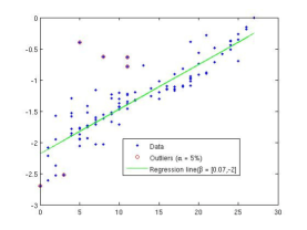
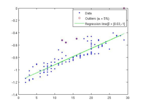
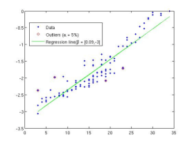
In this section, we discuss how our algorithm performs with respect to ground truths recorded. In our case, ground truths are the number of cars that are visible and handpicked for the correlation purposes. The results are shown in the Fig.2.

References

- [Benezeth et al., 2008] Benezeth, Y., Jodoin, P., Emile, B., Laurent, H., and Rosenberger, C. (2008). Review and evaluation of commonly-implemented background subtraction algorithms. In Pattern Recognition, 2008. ICPR 2008. 19th International Conference on, pages 1 –4.
- [Sheikh and Shah, 2005] Sheikh, Y. and Shah, M. (2005). Bayesian modeling of dynamic scenes for object detection. Pattern Analysis and Machine Intelligence, IEEE Transactions on, 27(11):1778–1792.
- [Stauffer and Grimson, 1999] Stauffer, C. and Grimson, W. (1999). Adaptive background mixture models for real-time tracking. In Computer Vision and Pattern Recognition, 1999. IEEE Computer Society Conference on., volume 2, pages 2 vol. (xxiii+637+663).