Comparing network covers using mutual information

Abstract

In network science, researchers often use mutual information to understand the difference between network partitions produced by community detection methods. Here we extend the use of mutual information to covers, that is, the cases where a node can belong to more than one module. In our proposed solution, the underlying stochastic process used to compare partitions is extended to deal with covers, and the random variables of the new process are simply fed into the usual definition of mutual information. With partitions, our extended process behaves exactly as the conventional approach for partitions, and thus, the mutual information values obtained are the same. We also describe how to perform sampling and do error estimation for our extended process, as both are necessary steps for a practical application of this measure. The stochastic process that we define here is not only applicable to networks, but can also be used to compare more general set-to-set binary relations.

1 Introduction

Many complex phenomena can be characterized by interconnected networks of basic parts: the network nodes. In order to gain in understanding of these complex phenomena, researchers often start by grouping nodes in non-overlapping modules, forming a so-called network partition. As there are many automatic ways of creating partitions from a raw network, partitions of the same network generated by different methods are frequently compared using one popular measure of similarity: the mutual information (MI)lancichinetti2009benchmarks ; barron1998minimum ; fortunato ; leung2009towards ; barber2009detecting ; ronhovde2009multiresolution ; berry2011tolerating . But partitions are not always the most appropiate way of defining functional components, as many phenomena can be better understood if, instead of partitions, the more general structure of cover is allowed, where modules of the network can overlap or form nested hierarchies. Researchers have developed methods that can automatically detect those structures stabeler2011using ; lancichinetti2011finding ; schaub2011coding ; kim2011map , but carrying along the mutual information as a similarity measure has proven more difficult, as we explain next.

When comparing two partitions, the mutual information is calculated by taking all the pairs of modules $(x,y)$, one from each partition, and counting the number of common nodes that these modules have. The count, divided by the total number of nodes in the network and denoted as $p(x,y)$, is used together with the fraction of nodes $p(x)$ and $p(y)$ that each of the modules $x$ and $y$ holds in its respective partition. These fractions are disguised as probabilities in the mutual information formulacover2006elements :

$$I(X;Y)=\sum_{y\in Y}\sum_{x\in X}p(x,y)\log_{2}\left(\frac{p(x,y)}{p(x)p(y)}\right).$$ (1)

We identify this way of calculating the MI as the counting approach.

We call two partitions or covers equivalent if they are different only in the choice of module’s names (Fig. 1). In the counting approach, if the two compared partitions are equivalent, the mutual information reaches a maximum value equal to the Shannon’s entropy of the fractions $p(x)$ and $p(y)$: $I(X;Y)=H(X)=H(Y)$. This happens because, for any two pair of modules $x$ and $y,$ either they contain exactly the same nodes, and thus $p(x,y)=p(x)=p(y)\neq 0$, or they have no common nodes at all and $p(x,y)=0$.

With covers, the problem is that it is not evident what to count: the fractions used by the counting approach don’t play well as probabilities any longer. For example, if one insists on using the fractions, the equality between MI and entropy won’t be valid for two equivalent covers (Fig 1).

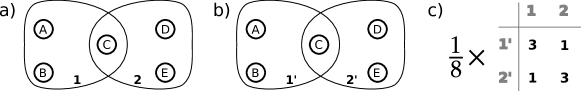
Figure 1: Why the counting approach can not be readily extended to covers. The cover in (a) is compared with itself (b); the only difference between the two subfigures is in module names ($\mathbf{1}$ and $\mathbf{2}$ vs $\mathbf{1^{\prime}}$ and $\mathbf{2^{\prime}}$). The number of common nodes for each pair of modules is shown in (c). Despite these two covers being equivalent with regard to node memberships, the mutual information (Eq. 1) calculated with the fractions from the counting approach is not equal to Shannon’s entropy.

Nonetheless, there are ways of comparing covers inspired by the mutual information. For example, the authors of lancichinetti2009benchmarks see a node belonging to a module as a yes-or-no fact, independent of everything else in the network and reflected on a binary vector. Starting from the concept of mutual information, they use this vector to ultimately produce a clustering-similarity measure. Being an approximation, expressions equivalent to Eq. 1 are used indirectly. Consequently, when their procedure is applied to singly-assigned nodes in partitions, the values obtained are not the same as in the conventional counting approach.

Here we take another course. For us, if a node is in many modules, we consider only one of those modules at a time, depending on an assumed context, such that different contexts can yield different node-module memberships. If we were talking about a person, for example, we would implicitly consider her part of a particular social group, depending on together with whom we mention her: a friend, a colleague, or a relative. We use this context principle to derive a stochastic process that disambiguates multiple memberships and yields module pairs, one single module from each cover and context. The probabilities of these pairs can be used straightforwardly in the mutual information formula (Eq. 1). Thus, we don’t require any changes to the mutual information definition, and our results are compatible with the counting approach. We call the obtained stochastic process extended.

The rest of this work is organized as follows. In section 2, we re-introduce the counting approach as a simple stochastic process, which justifies our intention of keeping it as a limit case when comparing covers which happen to be partitions. In section 3, we extend this stochastic process to covers. We complement section 3 with an Appendix that introduces the extended process using basic set theory, independet of the network concepts that we use in the main part of the paper. Section 4 shows that our extended process is sensitive to several kinds of differences between covers. Finally, in section 5 we explain how to control the error in the simulation procedure used to calculate our new measure.

2 Partitions and normalized MI

Here we show how comparing partitions is reduced to comparing random variables, and justify the counting approach conventionally used. In this and the following section, we will be assisted by a metaphor. In the metaphor, a caddie is choosing nodes with uniform probability from the network. Meanwhile, two players are in possession of each of the partitions. The players observe each node handled by the caddie, and announce the module that the node belongs to, according to their respective partition. The modules that each player reports are taken as the random variables $X$ and $Y$, whose probabilities we will use in the mutual information formula (Eq. 1). Because the caddie is drawing nodes with uniform probability, the probabilities of the random variables $X$ and $Y$ and the joint probability of any given pair can be calculated exactly as the proportion of nodes in each module and the fraction of nodes common to the pair of modules, respectively. Therefore, the counting approach can be framed as the MI of a stochastic process. We will call this stochastic process conventional, and we will keep it as a limit case occurring when we compare partitions using our extended process. We will define the extended process in the next section, but first, we will discuss the issue of normalization.

Normalization is required for getting a convenience indicator: one where 0 means no similarity and the value 1 is special because it means that the random variables are interchangeable, or, in our case, that the partitions or covers are equivalent. There are two ways in which normalization is normally donemcdaid2011normalized . In the first one, the mutual information is divided by the average of the Shannon’s entropies, while in the second one, it is divided by the maximum of the entropies. We advocate for using the maximum as the divisor because of the following. Suppose that four random variables $X$,$Y$,$Z$ and $W$ have Shannon’s entropies $H(X)=10$, $H(Y)=15$, $H(Z)=10$ and $H(W)=2$ . Furthermore, suppose the MI between $X$ and any other of the two variables is $2$. If the average is chosen as the divisor, the average-normalized MI between $X$ and the rest of the variables would be $\bar{I}_{a}(X;Y)=4/25$,$I_{a}(X;Z)=1/5$, $I_{a}(X;W)=1/3$. The variable $W$ gets a higher score than all of the others just because its entropy is lower, while $Z$ gets a higher score than $Y$ just because its entropy is similar to $X$’s. In other words, $Y$ is correctly penalized for overdescribing, but $W$ is wrongly rewarded for oversimplifying. Using the maximum entropy as a divisor, on the other hand, we would get instead $I_{n}(X;Y)=2/15$, $I_{n}(X;Z)=1/5$, and $I_{n}(X;W)=1/5$, which is more reasonable. Therefore we take the maximum as the divisor:

$$I_{n}(X;Y)=\frac{I(X;Y)}{\max\left\{H(X),H(Y)\right\}}$$ (2)

3 The stochastic process for covers

Here we look at how to extend the stochastic process defined in the previous section to cases where a node can belong to multiple modules. Appendix A complements this section with a shorter and conventional exposition of the same subject, suitable for readers familiar with very basic set theory.

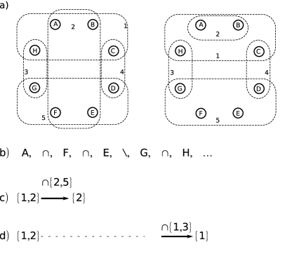
Figure 2: Illustration of how the new stochastic process works by looking at two example covers. Subfigure (a) shows the two covers, made by a common set of nodes A,B,C,D,E,F,G,H. Subfigure (b) shows an arbitrary interleaving of those nodes, alternating nodes and set operations. Subfigures (c) and (d) show the set operations outcome; the dotted portion of the line in subfigure (d) represents steps that do not remove modules, while the operations that contribute to the result are shown with a solid line.

In covers, a node can be associated with more than one module. When that happens, we use the context set by the memberships of other nodes to highlight just one module of the first node at a time. This is similar to a person associated with the groups family and work singling out the group work in the presence of colleagues.

In the players’ metaphor that we introduced before, this disambiguation mechanism allows the players to arrive at single modules, and, if the covers are equivalent, at matching answers. Because each player should be blind to what the other one does, he needs to base his actions on common information that he receives from the caddie.

We call our particular way of structuring this common information interleavings. Interleavings are the simplest representation of context that works with the membership relation between nodes and modules in a cover. Each interleaving consists of an ordered sequence of nodes, where between two consecutive nodes an operation bit is inserted. This bit represents the choice between one of two set operations: set intersection or set difference. Each node appears exactly once in the interleaving, so, when looking to the nodes alone, we see a permutation of nodes. As for the operation bits, they are randomly chosen with equal probability: taken alone they look like a random binary vector drawn from a uniform distribution. Figure 2(b) shows the first few elements of an example of interleaving, where the nodes have been represented with uppercase letters and the operation bits have been represented with the operation’s usual mathematical symbols.

Let’s see how a stochastic process can use the context provided by an interleaving to arrive at a unique module of the cover. Now, instead of handing nodes, the caddie produces an entire interleaving each time. When each player sees the first node of the interleaving, he will build a set with all the modules of that node, according to his cover. In the example of Fig. 2, both players get the set $\{1,2\}$. These sets will need to be disambiguated using the rest of the interleaving, and thus the players will keep them. If a player’s set contains only one module, he will output that module and finish. Otherwise, the player will use the next set operation and node from the interleaving. He uses the operation over his sets of modules and the incoming node’s set of modules. If the player gets a non-empty result, he will replace his set with this result set. In Fig. 2(c) we see that the first player can end almost inmediatly, using the modules that node $F$ has according to the first cover . However, as Fig. 2(d) shows, the other player has to keep going until he executes the intersection with the modules of node $H$. As long as no two modules in the same cover share exactly the same nodes, the process always ends in such a way that both players select a unique module. A proof of this is shown in Appendix B.

From this definition of the extended process, it is straightforward to use Eq. 2 to arrive at a value of the mutual information. The most efficient way of obtaining the probabilities for Eq. 2 is generating random interleavings with the computer and doing the disambiguation process described above. This is an approximate procedure, therefore, in section 5 we give additional details about how to perform the sampling and bound the error.

In summary, the differences between the conventional process and the extended one that we have introduced here, is that the first samples one node at a time, while the second exploits the context created by the rest of the node-module assignments in the network. As we hinted before, interleavings are just one of many possible structures. If a particular community detection method outputs more information associated with nodes or modules, that information could probably be put to good use. For example, it could influence the sampling of nodes or operations.

4 Behavior of the MI for cover differences

In the following sub-sections, we consider only a very basic aspect of the normalized mutual information (NMI): namely, that it is sensitive to differences in covers due to partition structure, hierarchies and/or overlaps.

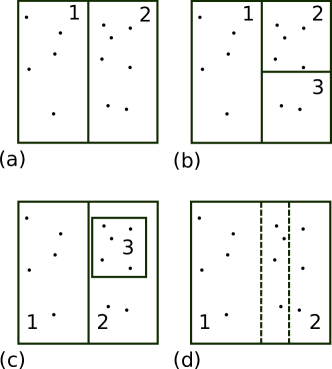
Figure 3: Several example covers. The reference cover in (a), is a partition made by two modules, denoted by 1 and 2, (b) shows a cover which is different just by splitting the previous one’s module 2 in two new modules: 2 and 3. In (c) a very simple hierarchy is shown, with module 3 containing some of the nodes of module 2. Finally, in (d) the nodes between the discontinuous line fringe belong (overlap) to both module 1 and 2. The comparison of the first partition with any of the other cases yields values of the NMI lower than 1.

The first thing to note is that, for any given partition $A$, its normalized mutual information with itself, according to both the conventional and the extended process will be 1. This property will remain valid for covers in general using the extended process.

Next we examine how this maximal value degrades when $A$ is compared with a cover which is obtained from $A$ according to some process: simple module division, introduction of a hierarchy, or introduction of overlapping modules.

4.1 Sensitivity to module splitting

If two partitions are compared, the values of the mutual information determined by both the conventional and the extended process are the same. That’s because the extended process will be able to decide an output module using just the first node from each interleaving. Therefore, the observations below will apply to both processes.

Given a partition $A$ , if $A^{\prime}$ is obtained from $A$ by splitting one of its clusters (see Fig. 3 (a) and (b) ), the mutual information between $A$ and $A^{\prime}$ will be the Shannon’s entropy of $A$, because $A^{\prime}$ determines $A$ completely; thus $H(A|A^{\prime})=0$ and $I(A;A^{\prime})=H(A)-H(A|A^{\prime})=H(A)$. However, normalization according to Eq. 2 will give the value

$$\frac{H(A)}{\max\{H(A),H(A^{\prime})\}}$$

and because $H(A^{\prime})>H(A)$, the NMI will be less than 1.

4.2 Sensitivity to introduction of hierarchies

We consider the case where the cover $A^{\prime}$ is obtained from $A$ by creating a new module with a subset of nodes, all of which are also already part of another module. In Fig. 3, an example would be subfigures (a) and (c). Because this case considers multiple modules per node, in this and the following sections we will be only speaking of the extended process.

We show that the comparison of $A$ and $A^{\prime}$ will result in decreased NMI. One of the conditions for an NMI of less than 1 is the one we exploited in the previous section: that the random variables have different entropy.

Let’s consider the outcome of the stochastic process for nodes of module 3 (and thus $1$) in Fig. 3 (c). These nodes belong to two modules, so the disambiguation process will consume more of the interleaving, and will yield either module $3$ or module $1$. In all those cases, the cover in Fig. 3(a) will still yield module $1$. So, the cover with hierarchies will produce a random variable with greater entropy than the partition in Fig. 3(a). However, because by looking to Fig.3 (c) one can always predict the outcome of the process for (a), these two covers again have the same mutual information, and the normalization in Eq. 2 will yield a value minor than 1. Therefore, the structure of the random variables for the extended process penalizes differences in hierarchies.

4.3 Sensitivity to introduction of overlaps

For overlaps, the mutual information itself is reduced: if we use the extended process over the covers in Fig. 3(a) and Fig. 3(d), upon seeing a node that belongs to module 2 in Fig. 3(d), it is not possible to determine unequivocally what will be the resulting module for the cover in Fig. 3(a). Thus, the MI between the two covers is less than the entropy of the partition in Fig. 3(a), and the obtained NMI value is less than 1.

5 Simulation and error control

The number of interleavings for the extended process grows very fast with the number of nodes and modules, so it is no longer practical to evaluate exactly the proportions of possible outcomes. But we can actually do the simulation with a computer program in an efficient way. That is, we can generate random interleavings and apply the disambiguation procedure described in section 3 and Appendix A, getting as many pair of modules as needed to reach a good estimate of the NMI. When we do the simulation process, the most likely outcomes will be, by definition, the ones with bigger contributions to the mutual information matrix $\left\{p(x,y)\right\}_{x\in X,y\in Y}$, and this will help us to bound the error.

We will call each individual act of choosing a random interleaving, applying the disambiguation procedure to it and getting a pair of modules an event. As explained before, we will count together events that yield the same pair of modules.

The NMI, as calculated by Eq. 2, is a function of the joint probabilities of events, denoted by $p(x,y)$. Also, the marginals $p(x)$ and $p(y)$, and the entropies $H(X)$ and $H(Y)$, are calculable from the joint probabilities. Because the joint probabilities are the basic input to all the calculations, it is convenient to rename them introducing variables $\theta_{1},\ldots\theta_{m}$ . Each $\theta_{i}$ denotes the true probability of an event yielding a particular pair of modules. This way, it is possible to write $I_{n}$ as a function application result $I_{n}=f\left(\theta_{1},\ldots\theta_{m}\right)$, where $f$ is given by equations 1 and 2.

We don’t have any of the true probability values $\theta_{i}$. Instead, we count the number $\zeta_{i}$ of events corresponding to $\theta_{i}$ , and the total number of events $N$ during the simulation: $N=\sum_{i=1}^{m}\zeta_{i}$. This count allows us to evaluate $f$ using frequencies, and obtain an estimate $\tilde{I}_{n}=f\left(\frac{\zeta_{1}}{N},\ldots\frac{\zeta_{m}}{N}\right)$ of the NMI. Because the value $\tilde{I}_{n}$ is a random variable, we can at best give a probabilistic estimate of the error $\left|\tilde{I}_{n}-I_{n}\right|$ . That is, given a risk $\epsilon$ and an error tolerance $e$, we simulate as many events $N$ as needed for

$$\textrm{Pr}\left(\left|\tilde{I}_{n}-I_{n}\right|<e\right)\geq 1-\epsilon$$ (3)

We need to relate the error $\left|\tilde{I}_{n}-I_{n}\right|$ with $\zeta_{1},\ldots,\zeta_{m}$ and $N$. If we consider $f$ as approximately linear inside of a small hypercube $\eta$ centered at $(\theta_{1},\ldots,\theta_{m})$ and spanning $\left|\theta_{i}-\frac{\zeta_{i}}{N}\right|$ in each dimension, we can get an approximation for $\left|\tilde{I}_{n}-I_{n}\right|$. Using first-order Tylor expansion and, in order to arrive at a worst case, taking absolute values, we get:

$$\left|\tilde{I}_{n}-I_{n}\right|\leq\sum_{i=1}^{m}\left|\frac{\partial I_{n}}{\partial\theta_{i}}\cdot\left(\frac{\zeta_{i}}{N}-\theta_{i}\right)\right|$$ (4)

In practice we replace$\left|\frac{\partial I_{n}}{\partial\theta_{i}}\cdot\left(\theta_{i}-\frac{\zeta_{i}}{N}\right)\right|$ by a finite difference equivalent:

$$\frac{\partial I_{n}}{\partial\theta_{i}}\cdot\left(\frac{\zeta_{i}}{N}-\theta_{i}\right)\leq\frac{\partial I_{n}}{\partial\theta_{i}}\cdot\left(\frac{\zeta_{i}}{N}-\theta_{i}^{\textrm{far}}\right)\approx\\ f(\frac{\zeta_{1}}{N},\ldots,\frac{\zeta_{i}}{N},\ldots\frac{\zeta_{m}}{N})-f(\frac{\zeta_{1}}{N},\ldots,\theta_{i}^{\textrm{far}},\ldots\frac{\zeta_{m}}{N})$$ (5)

where instead of $\theta_{i}$ we use a worst-case probability $\theta_{i}^{\textrm{far}}$. We say that this is a worst-case probability because it is the probability value farthest from $\frac{\zeta_{i}}{N}$ that would make the count $\zeta_{i}$ probable enough to satisfy the risk condition (Eq. 3).

To obtain $\theta_{i}^{\textrm{far}}$, we exploit the fact that each count $\zeta_{i}$ is approximately distributed following a binomial around the true probability: $\zeta_{i}\sim B\left(N,\theta_{i}\right)$. We assume a so-called component risk $\xi$, which we will shortly link to $\epsilon$, and solve the inverse problem of finding a $\theta_{i}^{\textrm{far}}$ such that:

$$\textrm{Prob}\left(X\leq\zeta_{i}\right)=\xi/2\\ \textrm{ given that }X\sim B(N,\theta_{i}^{\textrm{far}}).$$ (6)

This way, getting an event count in the interval between $\zeta_{i}$ and $N-\zeta_{i}$ will have probability $1-\xi$, according to $B(N,\theta_{i}^{\textrm{far}})$. When we account for all the variables $\zeta_{1},\ldots\zeta_{m}$, the probability of being inside the hypercube $\eta$ will be $(1-\xi)^{m}$. Equating this with the complement of our risk

$$1-\epsilon=(1-\xi)^{m}$$

and then doing first-order Taylor approximation assuming that $\epsilon$ is small enough, we obtain $\xi\approx\epsilon/m$. We can use this value of $\xi$ to solve for $\theta_{i}^{\textrm{far}}$ in Eq. 6. Then, substituting upwards in Eq. 5 and then in Eq. 4 we get the error’s upper bound. In this way, all that we need is to simulate enough events as for this error’s upper bound to fall below $e$.

6 Conclusions

We have defined a stochastic process that extends the use of mutual information to compare covers of networks and that in the limit case of network partitions yields the same results of the conventional process for partitions.

A notable characteristic of our extended process is that it only uses the membership relationships between nodes and modules. As appendix A shows, the extended process can be stripped from the network terminology and introduced instead using mathematical set-algebra. In other words, our extended process is not restricted to networks, but can be used to compare two binary set relations with a common finite domain.

There are many ways of defining similarity, and a single-number measure like ours can not possibly encompass all of them. Depending on what features researchers want to highlight when making comparisons, different measures must come into play. Nevertheless, the methodology of constructing random variables aware of the features that need to be compared, and then comparing the random variables using mutual information, can be adapted to more specific requirements.

We have made the source code of our implementation available at http://www.tp.umu.se/~alcides/.

Appendix A Formal definition of the extended process

This appendix extends the exposition in section 3 with formal notations and definitions.

The term “cover” that we used in the main text is just an alias for binary relation. That is, a cover $M$ is a binary relation between a finite set of “nodes” $E$ and a set of “modules” $L$. Using set notation: $M\subset E\times L$, where “$\times$” denotes Cartesian product. Given a node $e\in E$, we will use the term $\ell_{M}(e)$ to refer to the set of modules associated with $e$. That is, a module $l\in\ell_{M}(e)$ if and only if $(e,l)\in M$.

We define an interleaving $i_{E}$ of $E$ as the ordered sequence

$$i_{E}=[e_{0},b_{1},e_{1},\ldots,b_{\left\|E\right\|-1},e_{\left\|E\right\|-1}],$$

where $[e_{0},e_{1},\ldots e_{\left\|E\right\|-1}]$ forms a permutation of $E$ (that is, all the elements of $E$ in a particular order) and $b_{i}$ is either $0$ or $1$. We reserve the capital $I_{E}^{+}$ to denote the set of all posible interleavings with elements of $E$. Note that the cardinality of this set is $\left(\left\|E\right\|\right)!\times 2^{\left\|E\right\|-1}$.

For any given $M\subset E\times L$, we define a function $J_{M}$ that takes an interleaving and returns a subset of modules: $J_{M}:I_{E}^{+}\rightarrow\mathcal{P}(L)$. Here $\mathcal{P}(\cdot)$ denotes the power set of “$\cdot$”. We define $J_{M}\left([e_{0},b_{1},e_{1},\ldots,b_{\left\|E\right\|-1},e_{\left\|E\right\|-1}]\right)$ as the result $S_{\left\|E\right\|}$ of applying the following procedure: start with $S_{0}=\ell_{M}(e_{0})$. If $S_{k}$ has been calculated, calculate $S_{k+1}$ in the following way, for $k=0,1,2\ldots,\left\|E\right\|-1$

$$S_{k+1}=\begin{cases}s*&\textrm{if }s*\nsubseteq\emptyset\textrm{ and }b_{k}=1\\ s^{-}&\textrm{if }s^{-}\nsubseteq\emptyset\textrm{ and }b_{k}=0\\ S_{k}&\textrm{otherwise}\end{cases}$$ (7)

where

$$s*=S_{k}\bigcap\ell_{M}(e_{k})$$

and

$$s^{-}=S_{k}\setminus\ell_{M}(e_{k})$$

Note that $J_{M}\left([e_{0},b_{1},e_{1},\ldots,b_{\left\|E\right\|-1},e_{\left\|E\right\|-1}]\right)\subseteq\ell_{M}(e_{0})$. For our definition, we don’t need the entire set $I_{E}^{+}$, but rather the subset $I_{E,M}$ such that $i\in I_{E,M}$ if and only if $\left\|J_{M}(i)\right\|=1$. If an element $i$ belongs to $I_{E,M}$, we say that $J_{M}$ is well defined for $i$. In the next section we discuss under which conditions $I_{E}^{+}$ is equal to $I_{E,M}$.

Now it is straightforward to define the extended stochastic process: given two covers $M_{1}\subset E\times L_{1}$ and $M_{2}\subset E\times L_{2}$ over the same set of elements $E$, we assume the existence of a random variable with values over $I_{E}=I_{E,M_{1}}\bigcap I_{E,M_{2}}$ , such that all values of $I_{E}$ have the same probability. We can apply the functions $J_{M_{1}}$ and $J_{M_{2}}$ over $I_{E}$. The result are the modules $J_{M_{1}}(I_{E})$ and $J_{M_{2}}(I_{E})$, which in turn can be considered random variables over the set of modules $L_{1}$ and $L_{2}$. We define the MI of the two covers $M_{1}$ and $M_{2}$ as the mutual information between $J_{M_{1}}(I_{E})$ and $J_{M_{2}}(I_{E})$.

Appendix B Conditions under which the extended process yields only one module as response

The function $J_{M}$ defined in Appendix A may yield either a set with one element, or a set with more elements. In this Appendix, we prove that if every pair of modules of the cover is different regarding the nodes they contain, then the function $J_{M}$ will yield a set with just one element.

First we observe that the sequence of intermediate results defined by Eq. 7 and corresponding to a particular interleaving $[e_{0},b_{1}\ldots,b_{\left\|E\right\|-1},e_{\left\|E\right\|-1}]$ is non-increasing: $S_{k+1}$ will either have as many elements as $S_{k}$ or fewer, and evidently, $S_{k+1}\subseteq S_{k}$. Now we examine a final set $F=S_{\left\|E\right\|}$, whose cardinality is greater than 1. Because the family of sets $S_{k}$ is non-increasing, we have that $F\subset S_{k}$ for $k=0,1,\ldots,\left\|E\right\|-1$. If the set $F$ was conserved in all the $\left\|E\right\|-1$ operations prescribed by Eq. 7, it means that:

for set intersection operations:

$F$ was always present in the set $\ell_{M}(e_{k})$ for $k=1,\ldots e_{\left\|E\right\|-1}$ and thus not eliminated, or it was not present at all (in any of its members), and the operation was discarded because it resulted in the empty set.

for set difference operations:

$F$ was never present in the set $\ell_{M}(e_{k})$ for $k=1,\ldots e_{\left\|E\right\|-1}$ and thus not eliminated, or it was present but the operation was discarded because it resulted in an empty set. That means that all the elements of $F$ were in $\ell_{M}(e_{k})$.

These two branches converge in the fact that the set $F$ was always present or absent as a whole in each of the sets $\ell_{M}(e_{k})$ , and because each interleaving contains all the nodes, every module present in the set $F$ had exactly the same nodes.

References

- (1) A. Lancichinetti, S. Fortunato, Physical Review E 80(1), 16118 (2009)
- (2) A. Barron, J. Rissanen, B. Yu, Information Theory, IEEE Transactions on 44(6), 2743 (1998), ISSN 0018-9448
- (3) S. Fortunato, Phys. Rep. 486, 75 (2010)
- (4) I. Leung, P. Hui, P. Lio, J. Crowcroft, Physical Review E 79(6), 066107 (2009)
- (5) M. Barber, J. Clark, Physical Review E 80(2), 026129 (2009)
- (6) P. Ronhovde, Z. Nussinov, Physical Review E 80(1), 16109 (2009)
- (7) J. Berry, B. Hendrickson, R. LaViolette, C. Phillips, Physical Review E 83(5), 056119 (2011)
- (8) M. Stabeler, C. Lee, G. Williamson, P. Cunningham (2011)
- (9) A. Lancichinetti, F. Radicchi, J. Ramasco, PloS one 6(4), e18961 (2011)
- (10) M. Schaub, R. Lambiotte, M. Barahona, Arxiv preprint arXiv:1109.6642 (2011)
- (11) Y. Kim, H. Jeong, Physical Review E 84(2), 026110 (2011)
- (12) T. Cover, J. Thomas, Elements of information theory (wiley, 2006)
- (13) A. McDaid, D. Greene, N. Hurley, Arxiv preprint arXiv:1110.2515 (2011)