How to capture active particles

Abstract

For many applications, it is important to catch collections of autonomously navigating microbes and man-made microswimmers in a controlled way. Here we propose an efficient trap to collectively capture self-propelled colloidal rods. By means of computer simulation in two dimensions, we show that a static chevron-shaped wall represents an optimal boundary for a trapping device. Its catching efficiency can be tuned by varying the opening angle $\alpha$ of the trap. For increasing $\alpha$, there is a sequence of three emergent states corresponding to partial, complete, and no trapping. A trapping ‘phase diagram’ maps out the trap conditions under which the capture of self-propelled particles at a given density is rendered optimal.

One of the key survival strategies of human beings over the ages is their ability to catch animals. An efficient way to capture mammals, fish and birds is “trapping”, i.e. to release a device in a populated zone which then irreversibly attracts and stores the prey. While the methods for capturing (macroscopic) animals have been well-optimized by now, the corresponding problem in the micro-world, namely catching microbes, is much more challenging due to the strongly reduced nanometric size of the trap. The possibility to trap autonomously navigating microorganisms in a controlled way provides fascinating options to prevent or cure microbial contamination Redmond and Griffith (2003); Taylor et al. (2011) and to concentrate microbes near externally imposed patterned surfaces Galajda et al. (2007). Similar applications can be envisaged for man-made microswimmers, i.e. artificial particles which are actively propagating due to an internal “motor”. Examples include catalytically driven Janus particles Golestanian et al. (2005); Erbe et al. (2008); Palacci et al. (2010), colloids with artificial flagella Dreyfus et al. (2005); Tierno et al. (2008) and vibrated granulates Aranson and Tsimring (2006); Ramaswamy (2009). Lithographic techniques have been employed to confine, control and steer the motion of microbes and artificial microswimmers Kaehr and Shear (2009); Volpe et al. (2011). The use of lithographic nanopatterns has advanced significantly in recent years Englert et al. (2010); Mino et al. (2011) and has opened up numerous possibilities to sort particles Hulme et al. (2008); McCandlish et al. , to rectify their motion Galajda et al. (2007); Wan et al. (2008), and to design building blocks of micro-machines DiLeonardo et al. (2010); Sokolov et al. (2010); Angelani et al. (2009). Despite the experimental evidence there is little fundamental understanding of trapping phenomena in systems of active particles. This provides impetus for investigating the minimum requirements for designing efficient microbial traps and for unravelling the physical mechanisms responsible for collective trapping active particles.

Here, we propose an efficient scenario for capturing self-propelled rods by subjecting them to a static confining boundary of variable shape. The collective dynamics of the rods in confined geometry is explored by computer simulation using a two-dimensional, particle-resolved model for self-propelled colloidal rods. The presence of a boundary dramatically changes the collective dynamics of the rods, which in bulk show a strong propensity to form swarms, and induces collective self-trapping near the boundary. We show that a chevron-type (V-shaped) boundary represents the ideal geometry for an efficient microbial trap. The opening angle $\alpha$ of the chevron plays a key role in determing the self-trapping efficiency of the set-up. For increasing $\alpha$, the following sequence of non-equilibrium stationary states emerges: partial trapping, complete trapping, and no trapping. The transition from partial to complete trapping occurs smoothly at a lower critical opening angle while the complete trapping state abruptly terminates at an upper critical opening angle. The trapping phenomenon highlighted in this study is a collective effect which is driven by the many-body dynamics of self-motile rods in confinement. We show that the sharp transition from complete to incomplete trapping at higher critical opening angles has an appropriate system-size scaling which allows a classification similar to a true thermodynamic phase transition. The results of our simulation study are relevant for both two and three-dimensional systems of self-propelled particles. In three spatial dimensions the optimal shape of the trap would be a circular cone.

The model consists of a collection of $N$ active rods with length $\ell$ which experience a constant self-motile force $F_{a}$ directed along the main rod axis of each rod. Due to solvent friction the particles move in the overdamped low-Reynolds number regime, while interacting with the other particles and the boundary by steric forces only Wensink and Löwen (2008). The latter are implemented by discretizing the rod length into $n$ spherical segments and imposing a repulsive Yukawa potential between the segments of any two rods. The total potential between a rod pair $\{\alpha,\beta\}$ with orientational unit vectors $\{\hat{\bf u}_{\alpha},\hat{\bf u}_{\beta}\}$ and centre-of-mass distance ${\bf\Delta r}_{\alpha\beta}$ is then given by $U_{\alpha\beta}=(U_{0}/n^{2})\sum_{i=1}^{n}\sum_{j=1}^{n}\exp[-r_{ij}^{\alpha\beta}/\lambda]/r_{ij}^{\alpha\beta}$ where $U_{0}>0$ defines the amplitude, $\lambda$ the screening length and $r_{ij}^{\alpha\beta}=|{\bf\Delta r}_{\alpha\beta}+(l_{i}\hat{\bf u}_{\alpha}-l_{j}\hat{\bf u}_{\beta})|$ the distance between segement $i$ of rod $\alpha$ and $j$ of rod $\beta$ ($\alpha\neq\beta$) with $l_{i}=d(i-1)$, $i\in[1,n]$ denoting the segment position along the symmetry axis of the rod. The number of segments $n$ per rod is chosen such as to guarantee an intrarod segment-segment distance $d=\ell/(n-1)\leq\lambda$ to prevent rods from overlapping. A trap is introduced as a static boundary with a prescribed shape and contour length $\ell_{T}$. Particle-trap interactions are implemented by discretizing the trap boundary into $n_{T}=\lfloor\ell_{T}/d\rceil$ equidistant segments each interacting with the rod segments via the same Yukawa potential. Mutual rod collisions generate apolar nematic alignment which favor active liquid crystalline order, e.g. swarms, if the rod concentration exceeds a certain critical value. The boundary potential mimics a hard wall and imparts 2D planar order with rods pointing favorably perpendicular to the local wall normal.

In the overdamped regime, the equations of motion for the positions and orientations of the $N$-particle system in the absence of thermal noise emerge from a balance of the friction, interaction and self-propulsion forces and torques acting on each rod $\alpha$:

$${\bf f}_{\cal T}\cdot\partial_{t}{\bf r}_{\alpha}(t) = -\nabla_{{\bf r}_{\alpha}}U(t)+F_{a}\hat{\bf u}_{\alpha}(t),$$

$${\bf f}_{\cal{R}}\cdot\partial_{t}\hat{\bf u}_{\alpha}(t) = -\nabla_{\hat{\bf u}_{\alpha}}U(t),$$ (1)

in terms of the total potential energy $U=(1/2)\sum_{\alpha,\beta(\alpha\neq\beta)}U_{\alpha\beta}+\sum_{\alpha,T}U_{\alpha T}$ with $U_{\alpha T}$ the potential energy of rod $\alpha$ with the trap, and friction tensors ${\bf f}_{\cal T}=f_{\parallel}\hat{\bf u}\hat{\bf u}+f_{\perp}({\bf I}-\hat{\bf u}\hat{\bf u})$ and ${\bf f}_{\cal R}=f_{\cal R}{\bf I}$ (with ${\bf I}$ the 2D unit tensor). The Stokesian friction factors $f_{\parallel},f_{\perp},f_{\cal R}$ correspond to the parallel, perpendicular and rotational degrees of motion of a single rod and depend solely on the rod aspect ratio, defined as $a=\ell/\lambda$ Tirado et al. (1984). The self-propulsion speed of a single rod is simply $v_{0}=F_{a}/f_{\parallel}$ independent of time $t$ which is conveniently expressed in units $\tau=f_{\parallel}\lambda/F_{a}$, i.e. the time a free rod requires to traverse a distance equalling its length $\ell$.

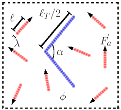
Figure 1: Sketch of a system of self-motile rods with aspect ratio $a=\ell/\lambda$ and axial active force $F_{a}$ at bulk density $\phi$ subjected to a static chevron-type trap with contour length $\ell_{T}$ and variable opening angle $\alpha$. The macroscopic system consists of periodic replicas with boundaries indicated by the dotted lines.

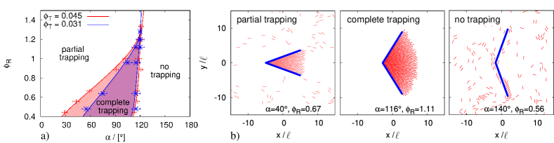
Figure 2: (a) ‘Phase diagram’ marking the three different trapping states for a chevron-type boundary with length $\ell_{T}=20\ell$; no trapping at large trap angle $\alpha$, complete trapping at medium angle and partial trapping at small angle upon variation of the reduced rod packing fraction $\phi_{R}=\phi/\phi_{T}$. Phase boundaries are shown for two different values of $\phi_{T}$; the area fraction occupied by the trap. The region of complete trapping is bounded by a triple point at larger rod concentration beyond which a smooth transition from no trapping to partial trapping occurs. (b) Snapshots depicting the three stationary states for the case $\phi_{T}=0.045$.

We simulate rods with aspect ratio $a=10$ in a rectangular simulation box with area $A$ and periodic boundary conditions in both Cartesian directions. A particle packing fraction is defined as $\phi=N\sigma/A$ with $\sigma=\ell\lambda+\lambda^{2}\pi/4$ the effective area of a single rod. In bulk these systems will spontaneously form polar nematic swarms with number density fluctuations being much stronger than for the (passive) equilibrium system at a comparable bulk density Narayan et al. (2007).

Let us now subject the swimmers to a V-shaped trap with contour length $\ell_{T}=20\ell$ and variable opening angle $0^{\circ}<\alpha<180^{\circ}$ (see Fig. 1). In the macroscopic limit, the system can be interpreted as a reservoir of microswimmers exposed to an equidistant array of mutually independent static traps. The area fraction occupied by the traps is angle-dependent with a maximum value given by $\phi_{T}=(\ell_{T}^{2}/8A)$, which fixes the number of rods via $N=(\ell_{T}^{2}/8\sigma)(\phi/\phi_{T})$. The trap area fraction shall be constrained to values below 0.1 in order to guarantee the traps to be completely independent of each other within the typical range of bulk rod packing fractions $0<\phi<0.1$ consider here. Trapped particles are identified by imposing a simple immobility criterion such that a particle is considered trapped if its velocity $v$ is below some threshold velocity $v^{\ast}$ ($v=|{\bf v}|<v^{\ast}$) during a long time interval of at least $t^{\ast}=25\tau$. This criterion suffices to disregard any particles that may be transiently anchored to the trap boundary. The number fraction of trapped rods defines the trapping efficiency $x_{T}(t)=N_{T}(t)/N$ and its long-time limit $x_{T}^{(0)}=\lim_{t\to\infty}x_{T}(t)$ ($0<x_{T}^{(0)}<1$) can be used to discern various stationary states.

Fig. 2a represents an overview of the collective trapping states that arise upon varying the two main system variables, the rod packing fraction $\phi$, and opening angle $\alpha$. The trapping ‘phase diagram’ exhibits three stationary regimes. First, for large $\alpha$ no trapping occurs as the cusp is too wide to efficiently capture a significant fraction of particles in the system. Second, below a certain critical angle a sharp transition towards complete trapping occurs. This state is characterized by the formation of a large monocluster in the cusp of the trap which contains all particles in the system. Upon further decreasing $\alpha$ a third region is entered corresponding to partial trapping. In this regime, the effective rod-trap collision cross-section is insufficient to trap all the particles present in the system, and a substantial portion of the rods remains mobile even at large $t$. The transition lines demarcating the various states in the diagram can be inferred from the evolution of the ‘order parameter’ $x_{T}^{(0)}$, i.e., the number fraction of trapped rods, as a function of the trap angle $\alpha$, as shown in Fig. 3a. Upon departing from the flat-wall limit ($\alpha\sim 180^{\circ}$) a sharp discontinuity occurs where $x_{T}^{(0)}$ jumps from zero to unity which signals a transition from no trapping to complete trapping. For sharper cusps (smaller $\alpha$) a second, continuous transition from complete to partial trapping can be located at the point where $x_{T}^{(0)}$ starts dropping smoothly below unity. The choice of the velocity cut-off $v^{\ast}=0.1v_{0}$, used in determining the trapping order parameter $x_{T}^{(0)}$, is robust as can be justified from the shape of the velocity histograms $P(v)$ in Fig. 3b where the markedly separated peaks provide an unambiguous distinction between immobile (trapped) particles and freely mov ing ones. From the histograms one can infer that the untrapped particles in the partial trapping state predominantly move freely with a maximum velocity $v_{0}$ whereas those in the no-trapping state are slowed down significantly due to collisions with the trap boundary.

It is worth noting from Fig. 2a that the transition from no trapping to complete trapping appears rather insensitive to the rod concentration as well the area fraction occupied by trap. Generically, complete trapping is possible only if the trap angle does not exceed a typical threshold value $\alpha\approx 120^{\circ}$. Moreover, by defining a reduced rod density $\phi_{R}=\phi/\phi_{T}$ the triple point is rendered virtually independent of the trap area fraction and attains a universal value $\phi_{R}^{\ast}\approx 1.3$. This suggests that the window of stability for complete trapping, as demarcated by the rod density $\phi^{\ast}$ at the triple point, can be systematically tuned by changing the number of traps per area and/or the contour length $\ell_{T}$ of the boundary. Although the state of complete-trapping is strictly suppressed at rod densities $\phi>\phi^{\ast}$, the trapping efficiency $x_{T}$ still shows a marked jump from zero to nearly 100% if the angle drops below about 120^∘. This indicates that the V-shaped boundary continues to be a powerful trapping device at larger rod densities.

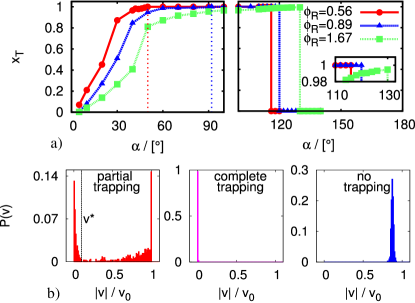
Figure 3: (a) Number fraction of trapped self-propelled rods $x_{T}^{(0)}=N_{T}(\infty)/N$ as a function of the opening angle $\alpha$ for three different reduced rod packing fractions $\phi_{R}$. The jumps around $\alpha=120^{\circ}$ signal ‘first-order’ phase transitions from no trapping to complete trapping. The dotted vertical lines in the left panel locate the transitions from complete to partial trapping upon decreasing $\alpha$. Inset: behaviour of $x_{T}$ near the critical trapping angle $\alpha\approx 120^{\circ}$. (b) Histograms of the normalized distribution $P(v)$ of particle velocities $v=|{\bf v}|$ corresponding to the three different states.

To ascertain whether the chevron is indeed the optimal shape we compare its trapping efficiency with that of a circular trap with identical trap area $A_{T}=52\ell^{2}$ and opening angle $\alpha=110^{\circ}$. A time series of the fraction of trapped particles reveals a distinct difference between the two trap shapes (Fig. 4). While the V-shape induces a fast intake of particles into the trap surface leading up to a trapping efficiency of almost 100% (complete trapping) at large times, the circular one fails to capture a significant fraction of particles over time. The rounded shape of the circular trap does not facilitate particle-wall anchoring but instead forces clusters of particles to slide collectively along the inner contour of the circular trap. This leads to a process whereby the rods collectively enter and leave the interior of the trap, as indicated by the ‘bursts’ in the number fraction of particles $x_{I}$ inside the trap in Fig. 4a. The rhythmic nature of the process is reflected by a peak in the power spectrum at a characteristic frequency which translates into a typical life time $212\tau$ of a rod cluster inside the circle trap. The number fraction of trapped (i.e. immobile) rods $x_{T}(t)$, however, remains practically zero throughout the sampled time interval in stark contrast to what is observed for the chevron trap.

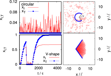
Figure 4: Comparison of the number fraction of particles $x_{I}$ located within the trap area and the fraction of immobile, trapped particles $x_{T}$ as a function of time $t$ for both V-shaped and circular traps with equal trap area $A_{T}=52\ell^{2}$, aperture angle $\alpha=110^{\circ}$ and reduced rod packing fraction $\phi_{R}=0.89$.

In conclusion, while there is a wealth of knowledge about trapping passive particles, e.g. colloids in optical tweezers or atoms in a Paul trap, there is considerable less understanding of capturing self-propelled particles. Here we have shown that active rods are efficiently self-trapped by a static chevron-type boundary. At the kink of the chevron, active particles are forced to oppose each other and form a jammed cluster which acts as a nucleus for capturing more particles until the whole trap area is filled. The opening angle of the trap plays a crucial role and its variation leads to three different emergent states corresponding to no trapping, complete trapping and partial trapping. A trap boundary which is rounded on the length scale of the particle extension is incapable of capturing particles over time. It is therefore essential that the trap boundary possesses at least one sharp cusp (whose size should be comparable to the rod length) which facilitates a fast build-up of clustered rods. The self-trapping mechanism is present in three spatial dimensions where the optimal trapping boundary is represented by a circular cone. We emphasize that the trapping mechanism proposed here is a collective, non-equilibrium effect which is conceptually different from trapping due to an equilibrium external force as represented by e.g. a deep potential well. In the equilibrium situation, collective trapping can be understood on the single-particle level. Moreover, geometric details of the trap boundary are usually irrelevant for understanding the global behaviour in contrast to the boundary-induced self-trapping mechanism advanced in this study.

The trapping phenomena presented here should be verifiable in experiments on rod-shaped bacteria Cisneros et al. (2007) or driven polar granular rods Volfson et al. (2004) exposed to geometrically structured boundaries Volpe et al. (2011); Englert et al. (2010); Mino et al. (2011). This set-up could, for instance, be exploited as an efficient purification device to manipulate and remove contaminating microbes. Future investigation will be aimed at comparing different types of propulsion mechanisms Gauger and Stark (2006); Götze and Gompper (2010) and the effect of the associated hydrodynamic flow fields generated by the collective particle motion in the presence of a static trap boundary Dhont (1996). We believe, however, that the hydrodynamic interactions will neither change the microscopic mechanism underpinning collective trapping nor the topology of the phase diagram presented here.