Cosmography from two-image lens systems: overcoming the lens profile slope degeneracy

Abstract

The time delays between the multiple images of a strong lens system, together with a model of the lens mass distribution, allow a one-step measurement of a cosmological distance, namely, the “time-delay distance” of the lens ($D_{\Delta t}$) that encodes cosmological information. The time-delay distance depends sensitively on the radial profile slope of the lens mass distribution; consequently, the lens slope must be accurately constrained for cosmological studies. We show that the slope cannot be constrained in two-image systems with single-component compact sources, whereas it can be constrained in systems with two-component sources provided the separation between the image components can be measured with milliarcsecond precisions, which is not feasible in most systems. In contrast, we demonstrate that spatially extended images of the source galaxy in two-image systems break the radial slope degeneracy and allow $D_{\Delta t}$ to be measured with uncertainties of a few percent. Deep and high-resolution imaging of the lens systems are needed to reveal the extended arcs, and stable point spread functions are required for our lens modelling technique. Two-image systems, no longer plagued by the radial profile slope degeneracy, would augment the sample of useful time-delay lenses by a factor of $\sim$$6$, providing substantial advances for cosmological studies.

1 Introduction

Since the discovery of the accelerated expansion of the Universe (Perlmutter et al., 1999; Riess et al., 1998), one of the key puzzles in cosmology has been the nature of dark energy which was proposed to explain the accelerated expansion. Recent studies based on various cosmological probes including the cosmic microwave background (CMB), supernovae, baryon acoustic oscillations, galaxy clusters, weak lensing, and gravitational lens time delays have shown that the Universe is consistent with dark energy being described by a cosmological constant $\Lambda$ (e.g., Komatsu et al., 2011; Conley et al., 2011; Suzuki et al., 2011; Reid et al., 2010; Blake et al., 2011; Mantz et al., 2010; Sehgal et al., 2011; Schrabback et al., 2010; Suyu et al., 2010). Nonetheless, Linder (2010) showed that current data provide little constraints on the properties and time evolution of dark energy when one relaxes the assumption that the dark energy equation of state, $w$, is constant (where $w=-1$ corresponds to the cosmological constant). To understand the nature of dark energy, a synergy of future observations of independent cosmological probes (to overcome the systematic effects in each approach), coupled with theoretical investigations of dark energy models, is needed.

In this paper, we focus on a particular cosmological probe: gravitational time delays in strong lens systems. By measuring the time delay(s) between the multiple images and modelling the mass distribution of the lens galaxy, one can infer the “time-delay distance”, $D_{\Delta t}$, to the lens system. This distance, which is a combination of angular diameter distances, is primarily sensitive to the Hubble constant ($D_{\Delta t}\propto H_{0}^{-1}$) but also depends on other cosmological parameters such as $w$. An accurate measurement of the Hubble constant with uncertainties better than a few percent provides the single most useful complement to results of the CMB for dark energy studies (e.g., Hu, 2005; Riess et al., 2009, 2011). Furthermore, time-delay lenses are also highly complementary to supernovae for determining the dark energy equation of state (Linder, 2011).

Suyu et al. (2010) showed that high-quality data of a four-image system allowed accurate lens mass modelling which yielded competitive cosmological constraints. On the other hand, analyses of two-image systems, which have significantly fewer time-delay and positional constraints on the mass model than four-image systems, are often plagued by model degeneracies and thus require model assumptions that may not be fully justified (e.g., Burud et al., 2002; Jakobsson et al., 2005; Paraficz et al., 2009). Ameliorating the shortcomings of two-image systems would provide significant advances to time-delay cosmography since there are currently more two-image systems than four-image systems (e.g., Oguri, 2007) and future large-scale surveys expect to discover about 6 times more two-image systems than four-image systems (e.g., Oguri & Marshall, 2010).

One of the main lens model limitations is due to the lens radial profile degeneracy: for a power-law mass distribution with three-dimensional density $\rho\propto r^{-\gamma^{\prime}}$, there is a strong degeneracy between the radial slope $\gamma^{\prime}$ and $D_{\Delta t}$. While studies of large strong lens samples from the Sloan Lens ACS Survey (SLACS) indicate that lenses are well described by a power law with $\gamma^{\prime}\sim 2.1$ (e.g., Koopmans et al., 2009; Auger et al., 2010; Barnabè et al., 2011), there is an intrinsic scatter in the slope of $\sim 0.15$. Furthermore, studies of higher redshift lens galaxies in the Strong Lensing Legacy Survey (SL2S) and the BOSS Emission-Line Lens Survey (BELLS) find an evolution in the lens profile slope where galaxies at higher redshift have shallower slopes (Ruff et al., 2011; Bolton et al., 2012). Both the intrinsic scatter and the evolution in the slope impact the $D_{\Delta t}$ measurement.

Witt et al. (2000) considered the time delays of power-law lens models with arbitrary angular structure, and showed that for non-isothermal mass distributions ($\gamma^{\prime}\neq 2$), the time delay depends in general on $D_{\Delta t}$, the image positions, $\gamma^{\prime}$ and the source position (or the lens potential). Wucknitz (2002) investigated further the power-law lens potentials with an additional external shear, and derived $D_{\Delta t}\propto\frac{3-\gamma^{\prime}}{\gamma^{\prime}-1}$ for fixed external shear (where we have converted the notation from $\beta\equiv 3-\gamma^{\prime}$ and $H_{0}$). This scaling is exact for power-law models with flexible angular structures that can fit perfectly to the observables, and is only approximate for elliptical models due to indirect dependencies of $D_{\Delta t}$ on $\gamma^{\prime}$ through, for example, the modelled source position. Instead of parametrising in terms of mainly the slope of the lens mass distribution, Kochanek (2002) showed that the time delays primarily depend on the average surface mass density in the annulus between the images $\langle\kappa\rangle$, in addition to $D_{\Delta t}$ and the image positions. When expressed in terms of $\langle\kappa\rangle$, the correction to the time delays from different values of $\gamma^{\prime}$ is small. The strong dependence of the time delays on the slope is incorporated indirectly through $\langle\kappa\rangle$. To highlight the full (both direct and indirect) dependence of $D_{\Delta t}$ on $\gamma^{\prime}$ and its impact on cosmography, we consider in the first part of the paper spherical power-law models. We also illustrate how one might constrain $\gamma^{\prime}$ with more lensing data than just the image positions from a single source, such as multiple compact source components or spatially extended sources.

By using the extended images of the lensed source in optical or near-infrared (NIR) wavelengths to model both the lens mass distribution and the source surface brightness distribution, studies have shown that the slope of the lens mass distribution can be constrained with uncertainties of a few percent in the annulus covered by the lensed images (e.g., Dye & Warren, 2005; Dye et al., 2008; Suyu et al., 2010; Vegetti et al., 2010). However, such studies focus mostly on four-image systems, and the use of extended two-image systems for cosmography has not been examined in detail. Furthermore, the lens systems that have been modelled so far using extended images in the optical/NIR wavelengths have relatively smooth variations in the image surface brightness. In contrast, the lensed sources in time-delay lenses typically have active galactic nuclei (AGNs) that are much brighter than the AGN host galaxies and thus require new modelling techniques to account for the large dynamical range in surface brightness.

The paper is organised as follows. In Section 2, we briefly review the method of gravitational lens time delays for cosmography. In Section 3, we consider a spherical power-law model to illustrate the degeneracy between $D_{\Delta t}$ and $\gamma^{\prime}$ and how one would break the degeneracy in principle. We simulate observations of two-image lens systems with spatially extended source galaxies in Section 4, and model these systems to test the recovery of $D_{\Delta t}$ in Section 5. Conclusions of our results are in Section 6.

2 Cosmography from gravitational lens time delays

In this section, we give a brief overview of using strong lens systems with measured time delays between the multiple images to study cosmology. More details on the subject can be found in, e.g., Schneider et al. (2006) and Treu (2010). Readers familiar with time-delay lenses may wish to proceed directly to Section 3.

According to Fermat’s principle, the multiple images in a strong lens system appear at locations where the travel times of the light paths are extrema or saddles. The excess time delay of an image at angular position $\mbox{\boldmath{${\theta}$}}=(\theta_{1},\theta_{2})$ with corresponding source position $\mbox{\boldmath{${\beta}$}}=(\beta_{1},\beta_{2})$ relative to the case of no lensing is

$$t(\mbox{\boldmath{${\theta}$}},\mbox{\boldmath{${\beta}$}})=\frac{D_{\Delta t}}{c}\left[\frac{(\mbox{\boldmath{${\theta}$}}-\mbox{\boldmath{${\beta}$}})^{2}}{2}-\psi(\mbox{\boldmath{${\theta}$}})\right],$$ (1)

where $c$ is the speed of light, and $D_{\Delta t}$ is the so-called time-delay distance that is a combination of the angular diameter distance to the lens/deflector ($D_{\rm d}$) at redshift $z_{\rm d}$, to the source ($D_{\rm s}$), and between the lens and the source ($D_{\rm ds}$):

$$D_{\Delta t}\equiv(1+z_{\rm d})\frac{D_{\rm d}D_{\rm s}}{D_{\rm ds}}.$$ (2)

The lens potential $\psi(\mbox{\boldmath{${\theta}$}})$ is related to the dimensionless surface mass density of the lens, $\kappa(\mbox{\boldmath{${\theta}$}})$, via

$$\nabla^{2}\psi(\mbox{\boldmath{${\theta}$}})=2\kappa(\mbox{\boldmath{${\theta}$}}).$$ (3)

For systems which have sources with intensities that vary in time such as active galactic nuclei (AGNs), one can monitor the intensities of the lensed images over time and measure the time delay, $\Delta t_{ij}$, between the images at positions $\mbox{\boldmath{${\theta}$}}_{i}$ and $\mbox{\boldmath{${\theta}$}}_{j}$:

$$\Delta t_{ij} \equiv t(\mbox{\boldmath{${\theta}$}}_{i},\mbox{\boldmath{${\beta}$}})-t(\mbox{\boldmath{${\theta}$}}_{j},\mbox{\boldmath{${\beta}$}})$$ (4)

$$= \frac{D_{\Delta t}}{c}\left[\frac{(\mbox{\boldmath{${\theta}$}}_{i}-\mbox{\boldmath{${\beta}$}})^{2}}{2}-\psi(\mbox{\boldmath{${\theta}$}}_{i})-\frac{(\mbox{\boldmath{${\theta}$}}_{j}-\mbox{\boldmath{${\beta}$}})^{2}}{2}+\psi(\mbox{\boldmath{${\theta}$}}_{j})\right].$$

By using the image configuration and morphology, one can model the mass distribution of the lens to determine the lens potential $\psi(\mbox{\boldmath{${\theta}$}})$ and the unlensed source position ${\beta}$. Lens systems with time delays can therefore be used to measure $D_{\Delta t}$ via equation (4) and constrain cosmological models (e.g., Refsdal, 1964, 1966; Fadely et al., 2010; Suyu et al., 2010). Since lens and source redshifts typically span between $z_{\rm d}\sim 0.1-1$ and $z_{\rm s}\sim 1-3$, respectively, an advantage of using the time-delay lenses for cosmography is that the method provides a one-step physical measurement of a cosmological distance $D_{\Delta t}$ independent of distance ladders.

3 Spherical Power-Law Lens: Illustration of the radial profile slope degeneracy

Previous studies of gravitational lenses show that power-law mass distributions provide adequate descriptions for lens galaxies (e.g., Koopmans et al., 2009; Suyu et al., 2009; Auger et al., 2010; Ruff et al., 2011; Barnabè et al., 2011). In this section, we explore the properties of a simple model: a spherical power-law mass distribution. Despite its simplicity, it clearly illustrates important parameter degeneracies, particularly between the time-delay distance and the radial slope.

3.1 Surface mass density, lens potential and deflection angle

A spherical power-law mass density distribution is of the form

$$\rho(r)=\rho_{0}r^{-\gamma^{\prime}},$$ (5)

where $\rho_{0}$ is the normalisation, $\gamma^{\prime}$ is the radial profile slope, $r=\sqrt{x^{2}+y^{2}+z^{2}}=\sqrt{R^{2}+z^{2}}$ is the three-dimensional radius, $R$ is the two-dimensional projected radius, and the $z$-axis is chosen to be the line-of-sight direction. An isothermal mass distribution has $\gamma^{\prime}=2$. The projected surface mass density along the line of sight is given by

$$\Sigma(R) = \int_{-\infty}^{+\infty}\rho(\sqrt{R^{2}+z^{2}})\,{\rm d}z$$ (6)

$$= \frac{\rho_{0}\sqrt{\pi}\,\Gamma(\frac{\gamma^{\prime}-1}{2})}{\Gamma(\frac{\gamma^{\prime}}{2})}\frac{1}{R^{\gamma^{\prime}-1}}.$$ (7)

The dimensionless surface mass density (also known as the convergence) for lensing studies is

$$\kappa(\vartheta)=\Sigma(\vartheta D_{\rm d})/\Sigma_{\rm cr},$$ (8)

where $\vartheta=R/D_{\rm d}$ and the critical surface mass density is

$$\Sigma_{\rm cr}=\frac{c^{2}D_{\rm s}}{4\pi GD_{\rm d}D_{\rm ds}}.$$ (9)

For convenience, we rewrite the dimensionless surface mass density as

$$\kappa(\vartheta)=\frac{3-\gamma^{\prime}}{2}\left[\frac{\theta_{\rm E}}{\vartheta}\right]^{\gamma^{\prime}-1}$$ (10)

by subsuming the normalisation constants into $\theta_{\rm E}$, which is also known as the “Einstein radius”. A point source that is located on the optic axis ($z$-axis) extending from the observer through the centre of the lens would be lensed into a ring with radius $\theta_{\rm E}$. This circle marks the tangential critical curve of the lens system, and the mass enclosed within the Einstein ring is

$$M_{\rm Ein} = \Sigma_{\rm cr}D_{\rm d}^{2}\left(2\pi\int_{0}^{\theta_{\rm E}}\kappa(\vartheta)\vartheta\rm{d}\vartheta\right)$$ (11)

$$= \Sigma_{\rm cr}D_{\rm d}^{2}\pi\theta_{\rm E}^{2}.$$ (12)

Note that the mass enclosed is directly dependent only on $\theta_{\rm E}$ and not on $\gamma^{\prime}$.

The lens potential corresponding to the $\kappa(\vartheta)$ in equation (10) can be obtained by solving equation (3) and is

$$\psi(\vartheta)=\frac{\theta_{\rm E}^{2}}{3-\gamma^{\prime}}\left(\frac{\theta_{\rm E}}{\vartheta}\right)^{\gamma^{\prime}-3}.$$ (13)

The scaled deflection angle is $\mbox{\boldmath{${\alpha}$}}(\mbox{\boldmath{${\theta}$}})=\mbox{\boldmath{${\nabla}$}}\psi(\mbox{\boldmath{${\theta}$}})$. For circularly symmetric surface mass densities ($\kappa(\mbox{\boldmath{${\theta}$}})=\kappa(\vartheta)$ where $\mbox{\boldmath{${\theta}$}}=\vartheta(\cos\,\varphi,\sin\,\varphi)$ in polar coordinates), the deflection angle becomes

$$\mbox{\boldmath{${\alpha}$}}(\mbox{\boldmath{${\theta}$}})=\alpha(\vartheta)\frac{\mbox{\boldmath{${\theta}$}}}{\vartheta}=\alpha(\vartheta)\hat{\mbox{\boldmath{${\theta}$}}},$$ (14)

(e.g., Schneider et al., 2006), and for the $\kappa(\vartheta)$ in equation (10), we have

$$\alpha(\vartheta)=\theta_{\rm E}\left(\frac{\theta_{\rm E}}{\vartheta}\right)^{\gamma^{\prime}-2}.$$ (15)

3.2 Lens systems with single component sources

Figure 1: Two-image lens system from a circularly symmetric lens mass distribution. The source (open circle) and images (filled circles) are collinear and are in the direction denoted by $\hat{\mbox{\boldmath{${\theta}$}}}$. The source position is at $\beta$ and the corresponding image positions are at $\theta_{\rm A}$ and $\theta_{\rm B}$.

Sources of time-delay lenses to date are AGNs with time-varying intensities. For practical purposes, the AGNs can be treated as point sources. The positions of the images of a source at position ${\beta}$ are obtained by solving the lens equation for ${\theta}$:

$$\mbox{\boldmath{${\beta}$}}=\mbox{\boldmath{${\theta}$}}-\mbox{\boldmath{${\alpha}$}}(\mbox{\boldmath{${\theta}$}}).$$ (16)

In the case where the lens mass distribution is spherically symmetric, the lens equation simplifies to

$$\beta=\theta-\alpha(\vartheta)\frac{\theta}{\vartheta},$$ (17)

where $\beta$ and $\theta$ are measured from the lens centre and are collinear. Note the distinction between $\theta$ and $\vartheta$, where $\vartheta=|\theta|$. For the deflection angle in equation (15), there are at most two non-central images of the source that appear when $\beta\lesssim\theta_{\rm E}$. Figure 1 is an illustration of such generic two-image systems from the spherical power-law model. The cross marks the location of the lens centre, and the two images are labelled by A and B. The unit vector $\hat{\mbox{\boldmath{${\theta}$}}}$ indicate the direction of line where the source (open circle) and the corresponding images (filled circles) lie. The source position is at $\beta$, and the image positions are at $\theta_{\rm A}$ and $\theta_{\rm B}$, where the lens centre is chosen to be the origin of the coordinates.

Given a two-image lens system as shown in Figure 1, we can use the image positions $\theta_{\rm A}$ and $\theta_{\rm B}$ to constrain the mass distribution of the lens system. In principle, the flux ratios of the images can also be used, but in practise, the time variability and delay between the images, substructure, microlensing and dust extinction affect the flux ratio significantly, leading to large uncertainties in the flux ratios. For simplicity, we consider only the image positions to probe the overall smooth component of lens mass distribution.

Assuming that the lens mass centre can be determined based on its light distribution, then the two image positions lead to the following set of constraint equations:

$$\left\{\begin{array}[]{l}\beta_{\rm s}=\theta_{\rm A}-\alpha(\vartheta_{\rm A})\frac{\theta_{\rm A}}{\vartheta_{\rm A}}=\theta_{\rm A}-\theta_{\rm E}\frac{\theta_{\rm A}}{\vartheta_{\rm A}}\left(\frac{\theta_{\rm E}}{\vartheta_{\rm A}}\right)^{\gamma^{\prime}-2}\\ \beta_{\rm s}=\theta_{\rm B}-\alpha(\vartheta_{\rm B})\frac{\theta_{\rm B}}{\vartheta_{\rm B}}=\theta_{\rm B}-\theta_{\rm E}\frac{\theta_{\rm B}}{\vartheta_{\rm B}}\left(\frac{\theta_{\rm E}}{\vartheta_{\rm B}}\right)^{\gamma^{\prime}-2}\\ \end{array}\right.$$ (18)

where we have substituted in equation (15). With three model parameters ($\beta_{\rm s}$, $\theta_{\rm E}$ and $\gamma^{\prime}$) and two constraints, the system of equations is underdetermined. The paucity of constraints from two-image systems explains why assumptions in the lens mass distributions such as mass following light, spherical symmetry and isothermality ($\gamma^{\prime}=2$) were often necessary in modelling two-image systems in the past (e.g., Vuissoz et al., 2007; Paraficz et al., 2009). Here, we explore the dependence of the model parameters and cosmological inferences on the slope $\gamma^{\prime}$ in the range of 1.5 to 2.5, which reflect the spread in the lens slopes from the SLACS, SL2S and BELLS samples (e.g., Koopmans et al., 2009; Auger et al., 2010; Barnabè et al., 2011; Ruff et al., 2011; Bolton et al., 2012). Since equations (18) cannot be solved analytically for generic values of $\gamma^{\prime}$, we consider six toy lens systems (I–VI) listed in Table 1 with different image configurations. The image positions are expressed in units of $\theta_{0}$ that sets the overall size of the lens system. We assume that $\vartheta_{\rm A}\geq\vartheta_{\rm B}$ and $\theta_{\rm A}>0$ (i.e., $\theta_{\rm B}<0$) without loss of generality.

Table 1: Two-image toy systems

System	$\theta_{\rm A}$ ($\theta_{0}$)	$\theta_{\rm B}$ ($\theta_{0}$)
I	1.0	$-1.0$
II	1.2	$-0.8$
III	1.2	$-0.7$
IV	1.4	$-0.7$
V	1.5	$-0.3$
VI	1.8	$-0.2$

Notes. Configuration of the six toy two-image lens systems. Columns 2 and 3 are the positions of images A and B in units of $\theta_{0}$.

We show in Figure 2 values of $\theta_{\rm E}$ and $\beta_{\rm s}$ that solve equations (18) for the range of slope values. For systems I to IV with nearly symmetric image configuration ($\vartheta_{\rm A}/\vartheta_{\rm B}\lesssim 2$), the value of $\theta_{\rm E}$ is quite insensitive to $\gamma^{\prime}$. This implies that the mass enclosed within $\theta_{\rm E}$ (which only has direct dependence on $\theta_{\rm E}$, as indicated in equation (12)) from strong lensing is accurate to within $\sim$$5\%$ for these systems. For the case with perfect symmetry ($\vartheta_{\rm A}=\vartheta_{\rm B}$) that has the source lensed into a ring, $\theta_{\rm E}$ is completely independent of $\gamma^{\prime}$ and the source is perfectly aligned with the lens ($\beta_{\rm s}=0$).

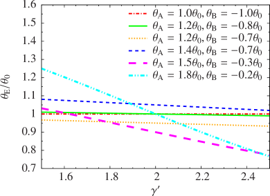
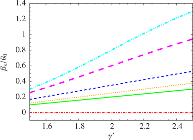
Figure 2: The Einstein radius ($\theta_{\rm E}$) and source position ($\beta_{\rm s}$) parameters for each of the six toy lens systems. For systems with images that are nearly symmetric with respect to the lens centre (i.e., $\vartheta_{\rm A}/\vartheta_{\rm B}\lesssim 2$), $\theta_{\rm E}$ is quite insensitive to lens profile slope $\gamma^{\prime}$.

3.3 Degeneracy between lens profile slope and $D_{\Delta t}$

The time delay between images B and A for circularly symmetric surface mass density follows from equation (4),

$$\Delta t_{\rm BA}=\frac{D_{\Delta t}}{c}\left[\frac{(\theta_{\rm B}-\beta_{\rm s})^{2}}{2}-\psi(\vartheta_{\rm B})-\frac{(\theta_{\rm A}-\beta_{\rm s})^{2}}{2}+\psi(\vartheta_{\rm A})\right].$$ (19)

For the power-law profile, the following property holds

$$\vartheta\alpha(\vartheta)=(3-\gamma^{\prime})\psi(\vartheta).$$ (20)

Using equations (18) and (20) in equation (19), we obtain the following relation between the time-delay distance and model parameters

$$\frac{D_{\Delta t}}{c\,\Delta t_{\rm BA}}=\frac{2(3-\gamma^{\prime})}{\gamma^{\prime}-1}\left[\theta_{\rm A}^{2}-\theta_{\rm B}^{2}+\frac{2(2-\gamma^{\prime})}{\gamma^{\prime}-1}\beta_{\rm s}(\vartheta_{\rm A}+\vartheta_{\rm B})\right]^{-1}.$$ (21)

This is consistent with equation (22) of Wucknitz (2002). We see in equation (21) that $D_{\Delta t}$ does not scale only as $\frac{3-\gamma^{\prime}}{\gamma^{\prime}-1}$ for the spherical power-law model due to the dependence of the quantities in the square brackets on $\gamma^{\prime}$ (both indirectly via $\beta_{\rm s}$ and directly). In Figure 3, we show the time-delay distance scaled by $\theta_{0}^{2}/c\,\Delta t_{\rm BA}$ as a function of $\gamma^{\prime}$ for Systems II to VI. System I is not shown since the source is lensed into a ring in this case so that the time delay between A and B is zero which provides no constraint on the $D_{\Delta t}$. In the bottom panel, we show the time-delay distance scaled relative to the isothermal case ($\gamma^{\prime}=2$). Lens systems with different image configurations lead to very similar relative time-delay distance. Furthermore, the relative $D_{\Delta t}$ depends sensitively on $\gamma^{\prime}$. Studies of the SLACS lens galaxies find a mean slope of $\gamma^{\prime}\sim 2.07$ with an intrinsic 1$\sigma$ scatter of $\sim$$0.15$ (Auger et al., 2010; Barnabè et al., 2011). A change of $\sim$$0.15$ in $\gamma^{\prime}$ corresponds to a rescaling of $D_{\Delta t}$ by $\sim$$15\%$. Therefore, the isothermal assumption that was frequently imposed in previous studies of two-image lenses would easily lead to a biased $D_{\Delta t}$ determination at the $10\%-20\%$ level. For precision cosmology, one must therefore measure accurately the slope of the lens mass profile. As seen earlier, systems with single-component sources cannot be used to constrain the slope via image positions alone (equations (18) are underdetermined). In the next section, we consider sources with two components.

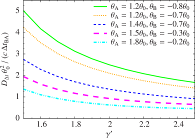
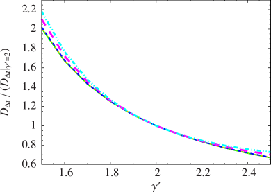
Figure 3: The time-delay distance as a function of the lens profile slope for systems with different image configurations. Top panel is the scaled time-delay distance, and the bottom panel is the time-delay distance relative to the isothermal ($\gamma^{\prime}=2$) case. The relative time-delay distance is very similar for all image configurations. An uncertainty in the slope of $0.15$, which is roughly the 1-$\sigma$ scatter in profile slopes of SLACS lenses, translates to an uncertainty of $\sim$$15\%$ on $D_{\Delta t}$, hindering cosmological studies.

3.4 Lens systems with two-component sources

In this section, we explore the constraints on the lens profile slope in systems where the source has two compact components. We label the image positions as $\theta_{\rm A1}$ and $\theta_{\rm B1}$ for the source component at position $\beta_{\rm s1}$, and as $\theta_{\rm A2}$ and $\theta_{\rm B2}$ for the source component at position $\beta_{\rm s2}$. Note that the two source components need not be collinear (in projection) with the lens centre. The four image positions lead to four constraint equations

$$\left\{\begin{array}[]{l}\beta_{\rm s1}=\theta_{\rm A1}-\theta_{\rm E}\frac{\theta_{\rm A1}}{\vartheta_{\rm A1}}\left(\frac{\theta_{\rm E}}{\vartheta_{\rm A1}}\right)^{\gamma^{\prime}-2}\\ \beta_{\rm s1}=\theta_{\rm B1}-\theta_{\rm E}\frac{\theta_{\rm B1}}{\vartheta_{\rm B1}}\left(\frac{\theta_{\rm E}}{\vartheta_{\rm B1}}\right)^{\gamma^{\prime}-2}\\ \beta_{\rm s2}=\theta_{\rm A2}-\theta_{\rm E}\frac{\theta_{\rm A2}}{\vartheta_{\rm A2}}\left(\frac{\theta_{\rm E}}{\vartheta_{\rm A2}}\right)^{\gamma^{\prime}-2}\\ \beta_{\rm s2}=\theta_{\rm B2}-\theta_{\rm E}\frac{\theta_{\rm B2}}{\vartheta_{\rm B2}}\left(\frac{\theta_{\rm E}}{\vartheta_{\rm B2}}\right)^{\gamma^{\prime}-2}\\ \end{array}\right.$$ (22)

With four equations and four unknowns ($\beta_{\rm s1}$, $\beta_{\rm s2}$, $\theta_{\rm E}$ and $\gamma^{\prime}$), the value of $\gamma^{\prime}$ can in principle be solved in the above system of equations (except for the special case where the two source components are located equidistant from the lens centre, so that the first two equations and the last two equations in (22) are equivalent up to a sign change).

We now explore the precision in which the image positions need to be measured in order to determine $\gamma^{\prime}$ of the lens to a few percent precision for cosmography. For illustrative purposes, we focus on lens system II in Table 1 and consider a range of possible image positions for the second component in the source that we assume to lie in the same direction from the lens centre as the first source component. In particular, we consider a range of values for $\theta_{\rm A2}-\theta_{\rm A1}$ spanning from $-0.4\theta_{0}$ to $0.2\theta_{0}$.

The top panel in Figure 4 quantifies the asymmetry in the image configurations relative to the lens galaxy for each of the $\theta_{\rm A2}-\theta_{\rm A1}$ values. The closer the ratio of the average image position (for the two-component images) is to 1, the more symmetric is the image configuration. For the case where $\theta_{\rm A2}-\theta_{\rm A1}=-0.4\theta_{0}$, there is perfect symmetry with $\theta_{\rm A1}=-\theta_{\rm B2}$ and $\theta_{\rm A2}=-\theta_{\rm B1}$ so that $\frac{|\theta_{\rm B1}+\theta_{\rm B2}|}{|\theta_{\rm A1}+\theta_{\rm A2}|}=1$ for all $\gamma^{\prime}$. In the bottom panel of Figure 4, we plot the relative image separation between the two image components as a function of $\gamma^{\prime}$. Apart from the case with $\theta_{\rm A2}-\theta_{\rm A1}=-0.4\theta_{0}$ (red dot-dashed lines), the derivative of the curves with respect to $\gamma^{\prime}$ is negative. Therefore, by measuring the relative separation between the images of different source components, one can measure $\gamma^{\prime}$ of the lens galaxy. The system with $\theta_{\rm A2}-\theta_{\rm A1}=-0.4\theta_{0}$ provides no information on $\gamma^{\prime}$ because in this perfectly symmetric image configuration, the second source component is on the opposite side and equidistant from the lens centre as the first source component, yielding effectively only a single component source in terms of constraints (which is insufficient for determining $\gamma^{\prime}$, as shown in Section 3.2).

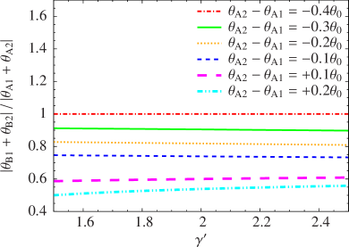
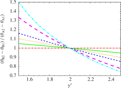
Figure 4: Configurations of images with 2-component sources. Top panel: asymmetry in the images, as defined by the ratio of the average image position of the two components. The ratio is 1 for perfect symmetry and is smaller for more asymmetric systems. Bottom panel: ratio of the separations between the images of the two components. For systems that are not perfectly symmetric, the curves are strictly monotonic, indicating that the slope can be determined in principle by measuring the image separations of the components.

In Figure 5, we show the derivative of $\theta_{\rm B2}-\theta_{\rm B1}$ with respect to $\gamma^{\prime}$. For typical systems with $\frac{|\theta_{\rm B1}+\theta_{\rm B2}|}{|\theta_{\rm A1}+\theta_{\rm A2}|}\gtrsim 0.7$ that are not perfectly symmetric, the derivative is $\sim$$0.04\theta_{0}$. Systems that are highly asymmetric ($\frac{|\theta_{\rm B1}+\theta_{\rm B2}|}{|\theta_{\rm A1}+\theta_{\rm A2}|}\lesssim 0.7$) can have larger magnitudes of $\sim$$0.1\theta_{0}$ for the derivatives. In order to measure $\Delta\gamma^{\prime}$ to within 0.03 (which translates to $\sim$$3\%$ in $D_{\Delta t}$), one would need to measure $\theta_{\rm B2}-\theta_{\rm B1}$ with accuracies better than $\sim$$0.1\theta_{0}\cdot 0.03=0.003\theta_{0}$. For typical galaxy-scale lenses with $\theta_{0}\sim 1^{\prime\prime}$, this requires $\lesssim$$3\,$milliarcsecond (mas) precision measurements on the separation between image components. Therefore, even though lenses with two-component sources can in principle be used to constrain the slope of the lens profile, in practise it would be difficult to measure the image separation between the components with mas precision to constrain $D_{\Delta t}$ with a few percent precision. Image positions of AGNs can be measured with mas precisions using radio telescopes, but usually the second source components (if any) are spatially extended radio jets whose positions are typically measured with precisions of several mas at best. There are, however, radio jets with compact knots that provide mas astrometries (e.g., Patnaik et al., 1995).

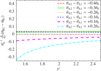
Figure 5: The derivative of the image separation between the two components ($\theta_{\rm B2}-\theta_{\rm B1}$) with respect to the slope $\gamma^{\prime}$. Highly asymmetric systems have larger magnitudes for the derivatives. To measure $\gamma^{\prime}$ to within $\sim$0.03 for precision cosmology, mas precision measurements in the relative image separation are required.

We have so far considered a power-law profile to describe the lens mass distribution. However, mass structures along the line of sight from us to the source typically induces shear on the system, which is characterised by a strength and an angle. Determining the external shear strength and angle in addition to the two power-law parameters ($\theta_{\rm E}$ and $\gamma^{\prime}$) and the two source positions ($\beta_{\rm s1}$ and $\beta_{\rm s2}$) is not possible since the images from the two-component sources provide only four constraints. Nonetheless, for typical two-image systems where the images lie on opposite sides with a small angular offset (i.e., no longer collinear with the lens galaxy) due to the presence of a general quadrupole (including external shear), the time delay depends weakly on the structure of the quadrupole (Kochanek, 2002). Therefore, the dependence of $D_{\Delta t}$ on $\gamma^{\prime}$ remains roughly the same in the presence of shear, but $\gamma^{\prime}$ becomes much more difficult to determine.

Systems with even more source components would provide additional constraints on the lens mass distribution (e.g., $\gamma^{\prime}$ and the external shear), but most systems do not have multiple compact source components with mas astrometries. Nonetheless, source galaxies (i.e., the hosts of the AGNs) are typically spatially extended, which can be thought of as many point sources with different intensities. The lensed images of the spatially extended sources form arcs, and the relative thickness of the arcs at various locations helps to constrain $\gamma^{\prime}$, just like the relative separation between $\theta_{\rm B2}-\theta_{\rm B1}$ and $\theta_{\rm A2}-\theta_{\rm A1}$, if measured accurately, constrains $\gamma^{\prime}$. While the arc thickness cannot be measured with mas precisions at a particular location even on current high-resolution imagings, the arc thickness can be measured at many angular positions. In the next sections we explore two-image lens systems with extended sources for cosmological studies.

4 Simulations

We simulate deep and high-resolution imaging of two-image lens systems that reveals the lensed arcs of the extended source galaxy. In particular, we simulate data that mimic the system HE1104$-$1805 (Wisotzki et al., 1993) with a lens redshift of 0.729 (Lidman et al., 2000) and a source redshift of 2.319 (Wisotzki et al., 1993; Smette et al., 1995). The corresponding time-delay distance for the lens is $D_{\Delta t}=4829\,{\rm Mpc}$ assuming a flat $\Lambda$CDM universe with $H_{0}=70\,{\rm km\,s^{-1}\,Mpc^{-1}}$ and $\Omega_{\Lambda}=0.72$. The time delay between the images is $162\pm 6$ days (Morgan et al., 2008).

4.1 Input lens mass profile and source light profile

To create simulated images and time delays for the mock systems, we use an elliptical power-law profile for the lens mass distribution with a constant external shear. The form of the elliptical power-law surface mass density that we employ is

$$\kappa_{\rm epl}(\theta_{1},\theta_{2})=\frac{3-\gamma^{\prime}}{1+q_{\rm d}}\left(\frac{\theta_{\rm E}}{\sqrt{\theta_{1}^{2}+\theta_{2}^{2}/q_{\rm d}^{2}}}\right)^{\gamma^{\prime}-1},$$ (23)

where $q_{\rm d}$ is the axis ratio of the elliptical isodensity contours, and $\theta_{\rm E}$ is the Einstein radius for the spherical-equivalent case (in the limit where $q_{\rm d}=1$, the above $\kappa_{\rm epl}$ distribution reduces to equation (10)). The deflection angle and lens potential can be computed following Barkana (1998). The distribution is suitably translated to the position of the lens galaxy (${\theta_{\rm c}}$) and rotated by the position angle ($\phi_{\rm d}$) of the lens galaxy (where $\phi_{\rm d}$ is measured counterclockwise from $\theta_{1}$).

We use the following form for the lens potential of the constant external shear in polar coordinates $\vartheta$ and $\varphi$:

$$\psi_{\rm ext}(\vartheta,\varphi)=\frac{1}{2}\gamma_{\rm ext}\vartheta^{2}\cos 2(\varphi-\phi_{\rm ext}),$$ (24)

where $\gamma_{\rm ext}$ is the shear strength and $\phi_{\rm ext}$ is the shear angle. The shear centre is arbitrary since it corresponds to an unobservable constant shift in the source plane. Note that $\kappa_{\rm ext}=\frac{1}{2}\nabla^{2}\psi_{\rm ext}$ is zero. The shear position angle of $\phi_{\rm ext}=0\degr$ corresponds to a shearing along the $\theta_{1}$-direction whereas $\phi_{\rm ext}=90\degr$ corresponds to a shearing in the $\theta_{2}$ direction.

For the surface brightness distribution of the AGN host galaxy in the source plane, we use Sérsic profiles with Sérsic index of 1 (corresponding to exponential profiles). Furthermore, we add a point source at the centre of the Sérsic profile to simulate the AGN.

4.2 Simulated WFC3 observations and Time Delays

We simulate Hubble Space Telescope (HST) imaging using the Wide Field Camera 3 (WFC3) in the infrared (IR) channel since the source galaxy is typically brighter in the infrared, providing better contrast with the AGN. The simulated image pixel size is $0.09^{\prime\prime}$, which can be dithered from images with the native pixel size of $0.13^{\prime\prime}$.

The steps for creating the simulated image are (1) generate an extended source intensity distribution with a central point source, (2) lens the source through the power-law and external shear profiles (described in Section 4.1) with parameters tuned to produce a high-resolution lensed image mimicking HE1104$-$1805, (3) convolve the lensed image with a subsampled point spread function (PSF) that is generated using the TinyTim software (Krist et al., 2011), (4) bin the convolved image to obtain an image pixel size of $0.09^{\prime\prime}$, and (5) add uniform Gaussian noise for the background (with $\sigma_{\rm bkgd}^{2}=1500$ counts, comparable to the level from a few orbits of HST observations) and Poisson noise for the source.

We consider three input values for the slope: $\gamma^{\prime}=1.8$, $\gamma^{\prime}=1.9$ and $\gamma^{\prime}=2.2$, and label them as Simulation #1, #2 and #3, respectively. For each input value, the other lens parameters and the point source position (of the AGN) are adjusted to create systems with the astrometry and time delay of HE1104$-$1805. For Simulations #1 and #2, we adopt a time-delay distance of $4829\,{\rm Mpc}$ (corresponding to the fiducial $\Lambda$CDM model) and can simulate time delays that are close to the observed delay in HE1104$-$1805. On the other hand, simulating a similar time delay with a much steeper slope of $\gamma^{\prime}=2.2$ requires a lower $D_{\Delta t}$ (as illustrated in Figure 3); consequently, we adopt $D_{\Delta t}=3263\,{\rm Mpc}$ for Simulation #3. In addition, Simulation #3 with a steeper mass profile has a lower lensing magnification in comparison to the other two simulations. Therefore, the intrinsic brightness and the size of the extended source in Simulation #3 are higher than those in the other two simulations so that the lensed images from the three simulations are similar in terms of arc thickness and signal-to-noise ratio. The position angle of the source is arbitrarily chosen to be either $0\degr$ or $90\degr$; based on Section 3.4, we suspect this quantity to be of little importance provided that the source is of sufficient spatial extent (for measuring the relative thickness of the lensing arcs). Table 2 summarises the crucial parameters and simulation outputs.

For each simulation of the slope, we also consider three different noise realisations. Specifically, we use different random number seed to generate the uniform Gaussian noise for the background and Poisson noise for the source. In Figure 6, we show the source and the WFC3 image of the first realisation of Simulation #1 in the right panels (top and bottom, respectively). The AGN is typically much brighter than the source/host galaxy, so only the AGN is conspicuous in these panels. We show in the left panels the source galaxy and the corresponding lensed image without the AGN to display the underlying extended arc features of the lensed AGN host galaxy (purely for illustration purposes without noise added). We model the simulated WFC3 image (bottom-right panel) in Section 5. For the lensed AGN, we adopt a typical uncertainty of 4 mas for the image positions and use $162\pm 6$ days for the time delay $\Delta t_{\rm AB}$.

Table 2: Simulation of Systems Resembling HE1104$-$1805

Parameter	Simulation #1	Simulation #2	Simulation #3
$\mbox{\boldmath{${\theta}$}}_{\rm c}$ (arcsec)	$(-0.955,-0.495)$	$(-0.960,-0.497)$	$(-0.955,-0.494)$
$\theta_{\rm E}$ (arcsec)	$1.406$	$1.333$	$1.462$
$q_{\rm d}$	$0.825$	$0.805$	$0.794$
$\phi_{\rm d}$ ($\degr$)	160	25	123
$\gamma^{\prime}$	1.8	1.9	2.2
$M_{\rm AGN}$	19.5	19.5	19.5
$M_{\rm host}$	23	23	22.5
$r_{\rm eff}$ (arcsec)	0.2	0.2	0.4
$q_{\rm s}$	0.8	0.8	0.8
$\phi_{\rm s}$ ($\degr$)	0	90	90
$\mbox{\boldmath{${\theta}$}}_{\rm A}$ (arcsec)	$\phantom{-}(0.000,-0.010)$	$\phantom{-}(0.000,-0.010)$	$\phantom{-}(0.000,-0.010)$
$\mbox{\boldmath{${\theta}$}}_{\rm B}$ (arcsec)	$(-2.910,-1.330)$	$(-2.910,-1.330)$	$(-2.910,-1.330)$
$D_{\Delta t}$ (Mpc)	4829	4829	3263
$\Delta t_{\rm AB}$ (days)	$164$	165	166

Notes. Input Lens and source parameters, and the simulated AGN positions and time-delays. The first five rows are the centroid ($\mbox{\boldmath{${\theta}$}}_{\rm c}$), strength ($\theta_{\rm E}$), axis ratio ($q_{\rm d}$), position angle ($\phi_{\rm d}$) and radial slope ($\gamma^{\prime}$) of the power-law mass distribution for the lens. The next five rows are the magnitude of the AGN ($M_{\rm AGN}$), the magnitude of the source host ($M_{\rm host}$), the effective radius ($r_{\rm eff}$), axis ratio ($q_{\rm s}$) and position angle ($\phi_{\rm s}$) of the Sérsic host. The next four rows are the two lensed image positions of the AGN ($\mbox{\boldmath{${\theta}$}}_{\rm A}$ and $\mbox{\boldmath{${\theta}$}}_{\rm B}$), the time-delay distance ($D_{\Delta t}$), and the time delay between the images ($\Delta t_{\rm AB}$).

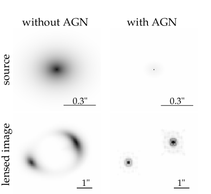
Figure 6: Simulated HST WFC3 image of Simulation #1. The left panels show the source galaxy (top) and the lensed image without noise (bottom) in the absence of the AGN in the source/host galaxy. The lensed image clearly exhibit the spatially extended arcs of the lensed AGN host galaxy. The right panels show the source and the lensed image in the presence of the AGN, which is typically much brighter than its host galaxy. We model the simulated WFC3 image with the AGN (bottom-right panel) in Section 5.

5 Breaking the $D_{\Delta t}$-slope degeneracy

In this section, we model the simulated images from the previous section with the aim to recover the time-delay distance for cosmography.

5.1 Lens and source model

To predict the image surface brightness and the time delays, we need to simultaneously model the lens mass distribution and the source surface brightness distribution. For the lens mass distribution, we use the same power law and external shear profiles as in equations (23) and (24). For notational simplicity, we collectively denote as ${\eta}$ the 6 power-law parameters ($\mbox{\boldmath{${\theta}$}}_{\rm c}$, $\theta_{\rm E}$, $q_{\rm d}$, $\phi_{\rm d}$, $\gamma^{\prime}$) and the 2 external shear parameters ($\gamma_{\rm ext}$, $\phi_{\rm ext}$). For the source surface brightness, we model the AGN light separately from the host to accommodate the large difference in size and brightness scales. We choose to model the lensed AGN as individual points on the image plane instead of a single point on the source plane. In the latter case, one can in principle solve for the predicted image positions and the image fluxes of a point source on the source plane for given values of the lens mass parameters (via equation (16) and the magnification dictated by the lens mass model). However, the observed image positions and especially the image fluxes of the point source could deviate from the macro (smooth power-law) model predictions due to substructure, microlensing, time delay and dust extinction; these effects could not be easily captured by a model that has the AGN as a point in the source plane. Since AGN image fluxes are typically anomalous (e.g., Dalal & Kochanek, 2002; Kochanek & Dalal, 2004), we model the fluxes of the lensed AGN images independently, but require that the image positions of the AGN are consistent with the macro model up to perturbations caused by, for example, substructures in the lens mass distribution (e.g., Chen et al., 2007). With the lensed AGN treated as individual points (before telescope blurring) and a model for the PSF, we have three parameters to describe each AGN image: position in $\theta_{1}$ and $\theta_{2}$ and an amplitude. We collectively denote the parameters for AGN light as ${\nu}$. For the spatially extended host of the AGN, we model its surface brightness on a grid of pixels (Suyu et al., 2006).

We express the predicted image of the lensed source as a vector of pixel intensities,

$$\mbox{\boldmath{${d}$}}^{\rm P}=\textbf{{B}}\textbf{{L}}(\mbox{\boldmath{${\eta}$}})\mbox{\boldmath{${s}$}}+\sum_{i=1}^{N_{\rm AGN}}\mbox{\boldmath{${a}$}}_{i}(\mbox{\boldmath{${\nu}$}}),$$ (25)

where B is the blurring operator to account for the PSF, $\textbf{{L}}(\mbox{\boldmath{${\eta}$}})$ is the lensing operator that maps source intensity to the image plane, ${s}$ is the vector of source pixel intensities (see, e.g., Suyu et al., 2006, 2009, for details), $N_{\rm AGN}$ is the number of AGN images, and $\mbox{\boldmath{${a}$}}_{i}(\mbox{\boldmath{${\nu}$}})$ is the vector of image pixel intensities for image $i$ of the AGN. This description assumes that the PSF is known a prior and is fixed. This is true in practise for HST images which have stable PSFs that can be modelled with sufficient accuracy based on instrumental setups and field stars.

To construct the likelihood function for the lens model using the pixel intensities, we also require an estimate of the intensity uncertainty at each pixel. Both the background (including sky and read noise) and the astrophysical source contribute to the noise in the intensity pixels. We have therefore two terms to describe the variance of the intensity at pixel $i$,

$$\sigma_{{\rm pix},i}^{2}=\sigma_{\rm bkgd}^{2}+fd_{i},$$ (26)

where $\sigma_{\rm bkgd}$ is the background uncertainty, $f$ is a scaling factor, and $d_{i}$ is the image intensity in counts. In the modelling, we adopt $\sigma_{\rm bkgd}^{2}=1500$  counts (input to the simulation) which can in practise be measured from a blank region in the image without astrophysical sources. The second term in equation (26), $fd_{i}$, corresponds to a scaled version of Poisson noise (with $f=1$ as the usual Poisson noise). The value of $f$ is chosen so that the reduced $\chi^{2}$ is $\sim$1 for the lensed image reconstruction (see, e.g., Suyu et al., 2006, for details on the computation of the reduced $\chi^{2}$). For a model where the PSF and the mass distribution are known perfectly, the usual Poisson noise with $f=1$ typically leads to a reduced $\chi^{2}\sim 1$. In practise, models are often simplified versions of reality so there could be residual features in the image reconstruction with a corresponding reduced $\chi^{2}$ that is $\gtrsim 1$. These residuals are frequently most prominent at locations where the intensities are high, such as at the positions of the AGN images. In this case, the model would try to reduce the high residual at a few localised locations (i.e., the AGN positions) instead of fitting to the overall structure of the data (i.e., the lensing arcs), which could lead to biased estimates of model parameters that are designed to characterise the global features. Increasing $f$ has the effect of downweighting these localised pixels with high $d_{i}$ and allowing the model to fit to the overall structure of the data. Furthermore, the increased $f$ value with an associated reduced $\chi^{2}\sim 1$ avoids underestimating the parameter uncertainty in simple models that are meant to characterise the large-scale features and not necessarily the small-scale features in the data (e.g., Brewer et al., 2012).

In sum, the parameters for our model are ${\eta}$, ${s}$ and ${\nu}$, and for simplicity, we fix the PSF to the input TinyTim PSF. Given a set of values for ${\eta}$ and ${\nu}$, the determination of the source surface brightness of the AGN host is a linear inversion (e.g., Warren & Dye, 2003; Suyu et al., 2006; Vegetti & Koopmans, 2009). Therefore, ${s}$ are known as linear parameters, and ${\eta}$ and ${\nu}$ are the nonlinear parameters.

5.2 Parameter Sampling and Priors

We model the simulated images and time delay with Glee that has been enhanced to incorporate AGN modelling. Since the AGN dominates the flux in the images, we first optimised for its position and amplitude while fixing the host flux to be zero. We then sample the posterior probability distribution function (PDF) of nonlinear parameters ${\eta}$ and ${\nu}$ with Markov chain Monte Carlo (MCMC) methods. We follow Dunkley et al. (2005) for efficient MCMC sampling and for assessing chain convergence.

Bayes’ Theorem states that the posterior PDF is

$$P(\mbox{\boldmath{${\eta}$}},\mbox{\boldmath{${\nu}$}}|\mbox{\boldmath{${d}$}},\Delta t)\propto P(\mbox{\boldmath{${d}$}},\Delta t|\mbox{\boldmath{${\eta}$}},\mbox{\boldmath{${\nu}$}})P(\mbox{\boldmath{${\eta}$}},\mbox{\boldmath{${\nu}$}}).$$ (27)

Since the imaging and time-delay data sets are independent, the likelihood separates:

$$P(\mbox{\boldmath{${d}$}},\Delta t|\mbox{\boldmath{${\eta}$}},\mbox{\boldmath{${\nu}$}})=P(\mbox{\boldmath{${d}$}}|\mbox{\boldmath{${\eta}$}},\mbox{\boldmath{${\nu}$}})P(\Delta t|\mbox{\boldmath{${\eta}$}},\mbox{\boldmath{${\nu}$}}).$$ (28)

The likelihood of the simulated WFC3 data, $P(\mbox{\boldmath{${d}$}}|\mbox{\boldmath{${\eta}$}},\mbox{\boldmath{${\nu}$}})$, is obtained by reconstructing the AGN host surface brightness distribution given values of ${\eta}$ and ${\nu}$, and marginalising over the source parameters ${s}$ (see, e.g., Suyu & Halkola, 2010, for details). Since the AGN images are modelled as independent points based on their surface brightness, we include an additional term to the likelihood to ensure that the lens model can reproduce the image positions. In particular, we multiply the original likelihood $P(\mbox{\boldmath{${d}$}}|\mbox{\boldmath{${\eta}$}},\mbox{\boldmath{${\nu}$}})$ by

$$\prod_{i}^{N_{\rm AGN}}\frac{1}{\sqrt{2\pi}\sigma_{i}}\exp\left[-\frac{|\mbox{\boldmath{${\theta}$}}_{i}-\mbox{\boldmath{${\theta}$}}^{\rm P}_{i}(\mbox{\boldmath{${\eta}$}})|^{2}}{2\sigma_{i}^{2}}\right],$$ (29)

where $\mbox{\boldmath{${\theta}$}}_{i}$ is the measured image position, $\sigma_{i}$ is the positional uncertainty that we adopt as 4 mas, and $\mbox{\boldmath{${\theta}$}}^{\rm P}_{i}$ is the predicted image position given the lens parameters. The likelihood for the time delay is given by

$$P(\Delta t|\mbox{\boldmath{${\eta}$}},\mbox{\boldmath{${\nu}$}})=\frac{1}{\sqrt{2\pi}\sigma_{\Delta t}}\exp\left[{-\frac{(\Delta t-\Delta t^{\rm P}(\mbox{\boldmath{${\eta}$}},\mbox{\boldmath{${\nu}$}}))^{2}}{2\sigma_{\Delta t}^{2}}}\right],$$ (30)

where $\Delta t$ is the measured time delay with uncertainty $\sigma_{\Delta t}$ and $\Delta t^{\rm P}$ is the predicted time delay computed via equation (4).

For the prior PDF $P(\mbox{\boldmath{${\eta}$}},\mbox{\boldmath{${\nu}$}})$, we assume uniform priors for ${\eta}$ and ${\nu}$ within physical ranges (e.g., axis ratio is uniform between 0 and 1) except for the centroid of the lens where we assume a Gaussian prior with width of $0.01^{\prime\prime}$ centred on the input values (which in practise would be obtained from the lens light distribution). For the pixelated source surface brightness distribution of the host, we consider both the curvature and gradient forms of regularisation/prior (see, e.g., Appendix A of Suyu et al., 2006).

5.3 Recovery of slope and $D_{\Delta t}$

We model the time delay and the simulated WFC3 image for each of the three realisations of the three simulations. To explore the effects of the different forms of regularisations for the source surface brightness, we adopt the curvature form for Simulations #1 and #2, and the gradient form for Simulation #3. In Figure 7, we show the source and image reconstruction of the AGN host surface brightness for the most probable lens and AGN parameters in the first realisation of Simulation #1. The noise level near the core of the lensed images is high due to the Poisson noise from the AGN. The modelled source resembles the input source in Figure 6 and reproduces the corresponding simulated lensed image.

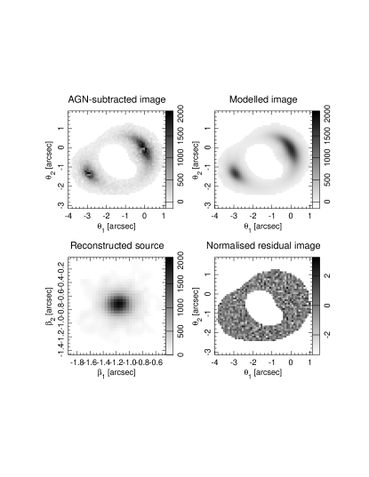
Figure 7: Image and source reconstruction of the first realisation in Simulation #1. Panels from top left in clockwise direction: image with AGN point images subtracted, modelled image, normalised image residual (in units of the uncertainty for each pixel), and the reconstructed AGN host galaxy.

In Figure 8, we show the joint PDF for $\gamma^{\prime}$ and $D_{\Delta t}$ after marginalising over all other parameters (source pixel intensities, AGN positions and amplitudes, power-law mass parameters and external shear) in each of the simulations/realisations. The cross indicates the input parameter value. The shapes and sizes of the credible regions are similar for the different realisations in each simulation. The orientations of the credible regions follow the degeneracy curves in Figure 3, and become more horizontal for simulations with higher $\gamma^{\prime}$. We recover the true $\gamma^{\prime}$ and $D_{\Delta t}$ values in Table 2 within the 99.7% (3$\sigma$) credible region for all cases, and within the 68.3% (1$\sigma$) credible region for approximately 2/3 of the cases as expected. By using the extended surface brightness of the host, we break the $D_{\Delta t}$-$\gamma^{\prime}$ degeneracy and recover $D_{\Delta t}$ to within $5\%$. Therefore, even though the width of the lensing arc cannot be measured to mas accuracy at any particular location given the image pixel size of $0.09^{\prime\prime}$, the thousands of image pixels collectively determine the relative thickness of the lensing arcs to sufficient accuracy for cosmography.

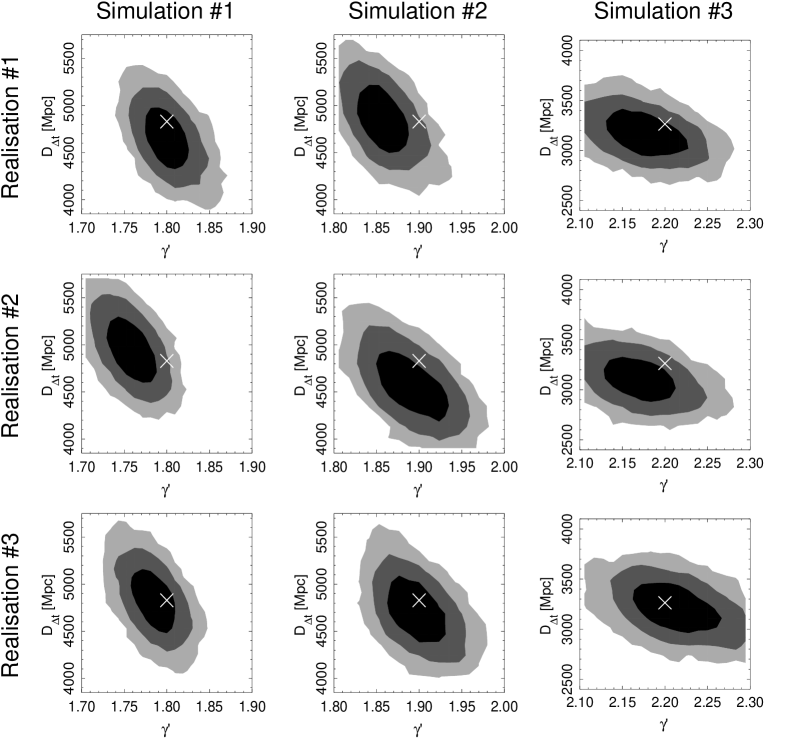
Figure 8: Marginalised PDF of $\gamma^{\prime}$ and $D_{\Delta t}$ for the three simulations (columns) with three realisations (rows) each. The three shaded areas show the 68.3%, 95.4% and 99.7% credible regions. The crosses mark the input values. By using the extended surface brightness of the AGN host, we break the degeneracy between $D_{\Delta t}$ and $\gamma^{\prime}$ and recover the input $D_{\Delta t}$ value within the uncertainties. Two-image lens systems with imaging that reveals the AGN host provide a robust cosmological distance probe.

5.4 Discussions

Our simulations demonstrate that two-image systems with detectable extended images of the AGN host provide accurate constraints on the time-delay distance, overcoming the radial profile slope degeneracy that has undermined this cosmological probe in the past. Only four-image lens systems or two-image lens systems with multi-component source structures (which have more observational constraints) have so far been shown to yield cosmological measurements that are not obviously dominated by systematic effects (e.g., Courbin et al., 2011; Suyu et al., 2010; Fadely et al., 2010; Wucknitz et al., 2004). Nonetheless, the majority of currently known time-delay lenses are two-image systems without multi-component sources (e.g., Oguri, 2007; Paraficz & Hjorth, 2010). Furthermore, future telescopes will find $\sim$$6$ times more two-image time-delay systems than four-image systems, and the Large Synoptic Survey Telescope (LSST) will discover thousands of two-image time-delay lenses (Oguri & Marshall, 2010). Therefore, effectively tapping into the abundant reservoir of two-image lenses will provide significant advances to time-delay cosmography.

The profile slope of interest for cosmography is actually the slope in the annulus between the images since the time delay primarily depends on the average surface mass density between the images (Kochanek, 2002). Therefore, even if the true lens mass distribution is not a global power law, it is well approximated by a local power law at the positions of the images. Other methods have probed the mass distribution in regions outside of the image annulus; for example, stellar kinematics of lens galaxies further constrain the mass distribution inside the effective radius of the lens galaxy (e.g., Koopmans & Treu, 2003; Treu & Koopmans, 2004; Koopmans et al., 2009; Barnabè et al., 2009; Auger et al., 2010; Barnabè et al., 2011; Sonnenfeld et al., 2011). In fact, stellar kinematics also help break the so-called “mass-sheet degeneracy” (Falco et al., 1985) in lensing (e.g., Grogin & Narayan, 1996; Koopmans et al., 2003; Suyu et al., 2010). Mass structures along the line of sight between the observer and the source (such as individual galaxies or groups/clusters of galaxies) contribute an external convergence, $\kappa_{\rm ext}$, to the lens mass distribution, and this external convergence is degenerate with $D_{\Delta t}$. Specifically, there is a mathematical transformation to the lens mass distribution, $\kappa\rightarrow(1-\kappa_{\rm ext})\kappa+\kappa_{\rm ext}$, which leaves the lensing observables (e.g., image positions/morphology, relative image fluxes and time delays) invariant but rescales $D_{\Delta t}$. A model that does not account for an existing $\kappa_{\rm ext}$ would underpredict or overpredict the value of $D_{\Delta t}$ for an overdense or underdense line of sight, respectively (by a factor of ($1-\kappa_{\rm ext}$)). Qualitatively, having a nonzero external convergence is analogous to adding an extra lens to the system which changes the focal length of the system, and hence the distance measurement. Both the radial profile slope degeneracy and the mass-sheet degeneracy are known to be the dominant sources of systematic uncertainties in measuring $D_{\Delta t}$. We have tackled and eliminated the radial profile slope degeneracy in this paper. Lens environment studies (e.g., Keeton & Zabludoff, 2004; Fassnacht et al., 2006; Momcheva et al., 2006; Fassnacht et al., 2011) in conjunction with stellar kinematics are effective in breaking the mass-sheet degeneracy (Suyu et al., 2010).

Our modelling of the lensed images requires a good knowledge of the PSF that is stable. Space-based imaging is ideal, but existing HST archival images of two-image lens systems that are not in cluster environments (which make $\kappa_{\rm ext}$ hard to control) do not have sufficient signal-to-noise ratio in the extended images of the AGN host galaxy for accurate modelling. Furthermore, most lens systems have been imaged with the Near Infrared Camera and Multi-Object Spectrometer (NICMOS) that have non-linear count rates; modelling these images, which have intensities of the extended AGN host galaxy that are severely contaminated by the bright AGNs, is prone to systematic effects. In contrast, WFC3 is a more sensitive and stable detector with a wider field of view (hence more field stars for PSF models) that would currently be the optimal instrument on HST to follow up the two-image lens systems for cosmography.

We have assumed in the model that the PSF is known perfectly, which is not true in practise. To explore the effect of imperfect PSF knowledge, we have also generated another TinyTim WFC3 PSF, located at approximately $45^{\prime\prime}$ from the original PSF, and used this offset PSF in the modelling step instead of the original PSF. This corresponds to the scenario where a star in the field is used to approximate the PSF at the location of the lens, which has been shown to work well for lens systems without bright AGNs in the spatially extended sources (e.g., Marshall et al., 2007; Suyu et al., 2009). In our case where the source AGN is bright, the PSF mismatch leads to imperfect AGN image modelling and consequently significant images residuals near the positions of the bright AGNs. As a result, the scaling factor $f$ in equation (26) is $\sim$8 for the offset PSF (whereas $f=1$ for the perfect PSF) to obtain a reduced image $\chi^{2}$ of $\sim$1 by downweighting these bright pixels with residuals that could otherwise cause biases in parameter estimations. Figure 9 shows the resulting constraints on $D_{\Delta t}$ and $\gamma^{\prime}$ (dashed) by using the offset PSF with the scaled pixel uncertainty in equation (26). The input $D_{\Delta t}$ and $\gamma^{\prime}$ are recovered without significant biases. In comparison to the case with a perfect PSF (shaded), the recovery of $D_{\Delta t}$ is degraded in precision from $\sim$$5\%$ to $\sim$$6\%$ (1$\sigma$, after marginalising over other parameters) due to the downweighting of high-residual pixels and the consequent loss of information in these pixels.

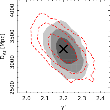
Figure 9: The effect of the PSF. Marginalised PDF of $\gamma^{\prime}$ and $D_{\Delta t}$ for Simulation #3 Realisation #3 modelled using the input TinyTim PSF (shaded) and a TinyTim PSF that is offset by $\sim$$45^{\prime\prime}$ from the input PSF (dashed). The three areas show the 68.3%, 95.4% and 99.7% credible regions. The cross marks the input values. With the imperfect (offset) PSF and the scaled pixel uncertainty in equation (26), the precision of the recovered $D_{\Delta t}$ is slightly degraded due to misfits near the bright AGN images.

For the simulated WFC3-IR images, we find that subsampling is necessary to avoid biases in the recovered parameters due to the large image pixel sizes. In other words, the predicted lensed image first need to be created and convolved on a finer resolution, then binned to the observed image resolution for calculating the likelihood. A subsampling factor of $\sim 3$ was sufficient to characterise both the PSF and the source intensity variation in the simulations.

In modelling the simulated images, a positional uncertainty of 4 mas was adopted for the AGN images and a Gaussian prior with width of $0.01^{\prime\prime}$ was imposed on the lens galaxy centroid. We consider the impact of relaxing these constraints individually to $0.09^{\prime\prime}$ (1 pixel) for observations where the positions cannot be easily measured (e.g., the lens galaxy is faint). We find that the credible regions in Figure 8 remain nearly the same if either the positional uncertainty of the AGN images or the prior on the lens galaxy centroid is relaxed to $0.09^{\prime\prime}$. This shows that the spatially extended arcs are providing most of the constraints on the mass distribution and the time-delay distance.

We have considered two types of source regularisations for the simulations (curvature for Simulations #1 and #2, and gradient for Simulation #3), and showed that the input $D_{\Delta t}$ and $\gamma^{\prime}$ are recovered irrespective of the choice in regularisation (Figure 8). For a given simulation, the two forms of regularisations lead to similar shapes and sizes of credible regions with slight shifts that are small compared to the size of the regions. Therefore, both forms of regularisations are viable options in modelling the extended arcs for typical AGN host galaxies that have smooth surface brightness distributions.

We have kept our simulations simple by excluding the light from the lens galaxy. In practise, the observed image would also contain lens light, which would affect the arc light and would need to be modelled as well. One way is to use Sérsic profiles to describe the lens light, and add another term to the right-hand side of equation (25) for the vector that describe the lens light intensities. The parameters for the Sérsic profiles are also nonlinear (like ${\eta}$ and ${\nu}$) and need to be sampled as well. A self-consistent model would simultaneously determine the lens light, the lens mass distribution, the AGN contribution, and the AGN host source surface brightness distribution. This is a high-dimensional nonlinear problem that is beyond the scope of this paper, and will be presented in a future study.

6 Conclusions

We have used the spherical power-law model to show that the time-delay distance depends sensitively on the slope, which cannot be constrained with a single-component compact source. A change in the slope of $\Delta\gamma^{\prime}\sim 0.15$, which is the typical scatter in lens galaxy slopes, leads to a $\sim 15\%$ change in $D_{\Delta t}$, undermining the use of two-image systems for accurate cosmological studies. Systems with two-component sources can be used to constrain the slope and derive useful cosmological constraints, but the relative separation between the images of the two components need to be measured with mas precision, which is difficult in practise. We use simulated HST images to test the usefulness of two-image systems with spatially extended arcs of the lensed AGN host galaxy. By simultaneously modelling the AGN light contribution, the lens mass profile, and the extended AGN host surface brightness distribution, we find that the relative thickness of the arcs accurately constrains the lens mass distribution and results in robust recovery of $D_{\Delta t}$ to a few percent. By establishing that two-image systems are no longer hindered by the radial profile slope degeneracy, the sample of useful time-delay lenses is enlarged by a factor of $\sim$$6$ which will provide substantial advances for cosmological studies.

References

- Auger et al. (2010) Auger M. W., Treu T., Bolton A. S., Gavazzi R., Koopmans L. V. E., Marshall P. J., Moustakas L. A., Burles S., 2010, ApJ, 724, 511
- Barkana (1998) Barkana R., 1998, ApJ, 502, 531
- Barnabè et al. (2011) Barnabè M., Czoske O., Koopmans L. V. E., Treu T., Bolton A. S., 2011, MNRAS, 415, 2215
- Barnabè et al. (2009) Barnabè M., Czoske O., Koopmans L. V. E., Treu T., Bolton A. S., Gavazzi R., 2009, MNRAS, 399, 21
- Blake et al. (2011) Blake C., Davis T., Poole G. B., Parkinson D., Brough S., Colless M., Contreras C., Couch W., et al. 2011, MNRAS, 415, 2892
- Bolton et al. (2012) Bolton A. S., Brownstein J. R., Kochanek C. S., Shu Y., Schlegel D. J., Eisenstein D. J., Wake D. A., Connolly N., et al. 2012, ArXiv e-prints (1201.2988)
- Brewer et al. (2012) Brewer B. J., Dutton A. A., Treu T., Auger M. W., Marshall P. J., Barnabè M., Bolton A. S., Koo D. C., Koopmans L. V. E., 2012, MNRAS, 422, 3574
- Burud et al. (2002) Burud I., Courbin F., Magain P., Lidman C., Hutsemékers D., Kneib J.-P., Hjorth J., Brewer J., et al. 2002, A&A, 383, 71
- Chen et al. (2007) Chen J., Rozo E., Dalal N., Taylor J. E., 2007, ApJ, 659, 52
- Conley et al. (2011) Conley A., Guy J., Sullivan M., Regnault N., Astier P., Balland C., Basa S., Carlberg R. G., et al. 2011, ApJS, 192, 1
- Courbin et al. (2011) Courbin F., Chantry V., Revaz Y., Sluse D., Faure C., Tewes M., Eulaers E., Koleva M., et al. 2011, A&A, 536, A53
- Dalal & Kochanek (2002) Dalal N., Kochanek C. S., 2002, ApJ, 572, 25
- Dunkley et al. (2005) Dunkley J., Bucher M., Ferreira P. G., Moodley K., Skordis C., 2005, MNRAS, 356, 925
- Dye et al. (2008) Dye S., Evans N. W., Belokurov V., Warren S. J., Hewett P., 2008, MNRAS, 388, 384
- Dye & Warren (2005) Dye S., Warren S. J., 2005, ApJ, 623, 31
- Fadely et al. (2010) Fadely R., Keeton C. R., Nakajima R., Bernstein G. M., 2010, ApJ, 711, 246
- Falco et al. (1985) Falco E. E., Gorenstein M. V., Shapiro I. I., 1985, ApJ, 289, L1
- Fassnacht et al. (2006) Fassnacht C. D., Gal R. R., Lubin L. M., McKean J. P., Squires G. K., Readhead A. C. S., 2006, ApJ, 642, 30
- Fassnacht et al. (2011) Fassnacht C. D., Koopmans L. V. E., Wong K. C., 2011, MNRAS, 410, 2167
- Grogin & Narayan (1996) Grogin N. A., Narayan R., 1996, ApJ, 464, 92
- Hu (2005) Hu W., 2005, 339, 215
- Jakobsson et al. (2005) Jakobsson P., Hjorth J., Burud I., Letawe G., Lidman C., Courbin F., 2005, A&A, 431, 103
- Keeton & Zabludoff (2004) Keeton C. R., Zabludoff A. I., 2004, ApJ, 612, 660
- Kochanek (2002) Kochanek C. S., 2002, ApJ, 578, 25
- Kochanek & Dalal (2004) Kochanek C. S., Dalal N., 2004, ApJ, 610, 69
- Komatsu et al. (2011) Komatsu E., Smith K. M., Dunkley J., Bennett C. L., Gold B., Hinshaw G., Jarosik N., Larson D., et al. 2011, ApJS, 192, 18
- Koopmans et al. (2009) Koopmans L. V. E., Bolton A., Treu T., Czoske O., Auger M. W., Barnabè M., Vegetti S., Gavazzi R., et al. 2009, ApJ, 703, L51
- Koopmans & Treu (2003) Koopmans L. V. E., Treu T., 2003, ApJ, 583, 606
- Koopmans et al. (2003) Koopmans L. V. E., Treu T., Fassnacht C. D., Blandford R. D., Surpi G., 2003, ApJ, 599, 70
- Krist et al. (2011) Krist J. E., Hook R. N., Stoehr F., 2011, in Kahan M. A., ed., Optical Modeling and Performance Predictions V Proc. of SPIE Vol. 8127. p. 1
- Lidman et al. (2000) Lidman C., Courbin F., Kneib J.-P., Golse G., Castander F., Soucail G., 2000, A&A, 364, L62
- Linder (2010) Linder E. V., 2010, ArXiv e-prints
- Linder (2011) Linder E. V., 2011, Phys.Rev.D, 84, 123529
- Mantz et al. (2010) Mantz A., Allen S. W., Rapetti D., Ebeling H., 2010, MNRAS, 406, 1759
- Marshall et al. (2007) Marshall P. J., Treu T., Melbourne J., Gavazzi R., Bundy K., Ammons S. M., Bolton A. S., Burles S., Larkin J. E., Le Mignant D., Koo D. C., Koopmans L. V. E., Max C. E., Moustakas L. A., Steinbring E., Wright S. A., 2007, ApJ, 671, 1196
- Momcheva et al. (2006) Momcheva I., Williams K., Keeton C., Zabludoff A., 2006, ApJ, 641, 169
- Morgan et al. (2008) Morgan C. W., Eyler M. E., Kochanek C. S., Morgan N. D., Falco E. E., Vuissoz C., Courbin F., Meylan G., 2008, ApJ, 676, 80
- Oguri (2007) Oguri M., 2007, ApJ, 660, 1
- Oguri & Marshall (2010) Oguri M., Marshall P. J., 2010, MNRAS, 405, 2579
- Paraficz & Hjorth (2010) Paraficz D., Hjorth J., 2010, ApJ, 712, 1378
- Paraficz et al. (2009) Paraficz D., Hjorth J., Elíasdóttir Á., 2009, A&A, 499, 395
- Patnaik et al. (1995) Patnaik A. R., Porcas R. W., Browne I. W. A., 1995, MNRAS, 274, L5
- Perlmutter et al. (1999) Perlmutter S., Aldering G., Goldhaber G., Knop R. A., Nugent P., Castro P. G., Deustua S., Fabbro S., et al. 1999, ApJ, 517, 565
- Refsdal (1964) Refsdal S., 1964, MNRAS, 128, 307
- Refsdal (1966) Refsdal S., 1966, MNRAS, 132, 101
- Reid et al. (2010) Reid B. A., Percival W. J., Eisenstein D. J., Verde L., Spergel D. N., Skibba R. A., Bahcall N. A., Budavari T., et al. 2010, MNRAS, 404, 60
- Riess et al. (1998) Riess A. G., Filippenko A. V., Challis P., Clocchiatti A., Diercks A., Garnavich P. M., Gilliland R. L., Hogan C. J., et al. 1998, AJ, 116, 1009
- Riess et al. (2011) Riess A. G., Macri L., Casertano S., Lampeitl H., Ferguson H. C., Filippenko A. V., Jha S. W., Li W., Chornock R., 2011, ApJ, 730, 119
- Riess et al. (2009) Riess A. G., Macri L., Casertano S., Sosey M., Lampeitl H., Ferguson H. C., Filippenko A. V., Jha S. W., et al. 2009, ApJ, 699, 539
- Ruff et al. (2011) Ruff A. J., Gavazzi R., Marshall P. J., Treu T., Auger M. W., Brault F., 2011, ApJ, 727, 96
- Schneider et al. (2006) Schneider P., Kochanek C. S., Wambsganss J., 2006, Gravitational Lensing: Strong, Weak and Micro (Springer)
- Schrabback et al. (2010) Schrabback T., Hartlap J., Joachimi B., Kilbinger M., Simon P., Benabed K., Bradač M., Eifler T., et al. 2010, A&A, 516, A63
- Sehgal et al. (2011) Sehgal N., Trac H., Acquaviva V., Ade P. A. R., Aguirre P., Amiri M., Appel J. W., Barrientos L. F., et al. 2011, ApJ, 732, 44
- Smette et al. (1995) Smette A., Robertson J. G., Shaver P. A., Reimers D., Wisotzki L., Koehler T., 1995, A&AS, 113, 199
- Sonnenfeld et al. (2011) Sonnenfeld A., Treu T., Gavazzi R., Marshall P. J., Auger M. W., Suyu S. H., Koopmans L. V. E., Bolton A. S., 2011, ArXiv e-prints (1111.4215)
- Suyu & Halkola (2010) Suyu S. H., Halkola A., 2010, A&A, 524, A94
- Suyu et al. (2011) Suyu S. H., Hensel S. W., McKean J. P., Fassnacht C. D., Treu T., Halkola A., Norbury M., Jackson N., et al. 2011, ArXiv e-prints (1110.2536)
- Suyu et al. (2010) Suyu S. H., Marshall P. J., Auger M. W., Hilbert S., Blandford R. D., Koopmans L. V. E., Fassnacht C. D., Treu T., 2010, ApJ, 711, 201
- Suyu et al. (2009) Suyu S. H., Marshall P. J., Blandford R. D., Fassnacht C. D., Koopmans L. V. E., McKean J. P., Treu T., 2009, ApJ, 691, 277
- Suyu et al. (2006) Suyu S. H., Marshall P. J., Hobson M. P., Blandford R. D., 2006, MNRAS, 371, 983
- Suzuki et al. (2011) Suzuki N., Rubin D., Lidman C., Aldering G., Amanullah R., Barbary K., Barrientos L. F., Botyanszki J., et al. 2011, ArXiv e-prints (1105.3470)
- Treu (2010) Treu T., 2010, ARA&A, 48, 87
- Treu & Koopmans (2004) Treu T., Koopmans L. V. E., 2004, ApJ, 611, 739
- Vegetti & Koopmans (2009) Vegetti S., Koopmans L. V. E., 2009, MNRAS, 392, 945
- Vegetti et al. (2010) Vegetti S., Koopmans L. V. E., Bolton A., Treu T., Gavazzi R., 2010, MNRAS, 408, 1969
- Vuissoz et al. (2007) Vuissoz C., Courbin F., Sluse D., Meylan G., Ibrahimov M., Asfandiyarov I., Stoops E., Eigenbrod A., et al. 2007, A&A, 464, 845
- Warren & Dye (2003) Warren S. J., Dye S., 2003, ApJ, 590, 673
- Wisotzki et al. (1993) Wisotzki L., Koehler T., Kayser R., Reimers D., 1993, A&A, 278, L15
- Witt et al. (2000) Witt H. J., Mao S., Keeton C. R., 2000, ApJ, 544, 98
- Wucknitz (2002) Wucknitz O., 2002, MNRAS, 332, 951
- Wucknitz et al. (2004) Wucknitz O., Biggs A. D., Browne I. W. A., 2004, MNRAS, 349, 14