Generating Functionals of Random Packing Point Processes: From Matérn to $\infty$-Matérn

Abstract

In this paper we study the generating functionals of several random packing processes: the classical Matérn hard-core model; its extensions, the $k$-Matérn models and the $\infty$-Matérn model, which is an example of random sequential packing process. We first give a sufficient condition for the $\infty$-Matérn model to be well-defined (unlike the other two, the latter may not be well-defined on unbounded spaces). Then the generating functional of the resulting point process is given for each of the three models as the solution of a differential equation. Series representations and bounds on the generating functional of the packing models are also derived. Last but not least, we obtain moment measures and Palm distributions of the considered packing models departing from their generating functionals.

1 Introduction

Random packing models (RPM) are point processes (p.p.s) where points ”contending” with each other cannot be simultaneously present. These p.p.s play an important role in many studies in physics, chemistry, material science, forestry and geology. The first use of RPMs is to describe systems with hard-core interactions. The most important applications are reactions on polymer chains [1], chemisorption on a single-crystal surface [2], and absorption in colloidial systems [3]. In these models, each point (molecule, particle,$\cdots$) in the system occupies some space, and two points with overlapping occupied space contend with each other. Another example is the study of seismic and forestry data patterns [4], where RPMs are used as a reference model for the data sets under consideration.
Recently, the study of wireless communications by means of stochastic geometry gave rise to another type of application. In wireless communications, each point (node, user, transmitter,$\cdots$) does not occupy space but instead generates interference to other points [5, 6]. Two points contend if either of them generates too much interference to the other. The present paper is mainly motivated by this kind of application. Nevertheless, the models we consider here are quite general and can be applied to other contexts. In particular, we will study here:

• The Matérn “hard-core“ model: this is one of the classical models in the study of packing processes. Defined by Matérn in [7] as the type II model and now usually referred to as the Matérn hard-core model, one can think of it as a dependent thinning of a Poisson p.p. $\Phi$, which is called the proposed p.p. The contention between two proposed points is determined by a contention mechanism. In the original setting, this consists in letting each proposed point $x$ occupy a ball $B(x,r)$ of radius $r$ centered at $x$. Two points with overlapping balls, or equivalently, with Euclidian distance smaller than $2r$, contend with each other. Once the contention between points is determined, a retention mechanism is used to prohibit the simultaneous presence of any two contending points. This mechanism assigns a uniform independent random mark $t(x)$ in $[0.1]$ to each proposed point $x$. A point is retained iff it has the smallest mark among its contenders.
  There are many extensions of the original Matérn model, all of which consist in generalizing the contention mechanism whilst keeping the retention mechanism unchanged. The first extension of this kind is the ”soft-core” model which randomizes the parameter $r$. Each proposed point $x$ occupies a ball $B(x,r(x))$ of random radius $r(x)$. Two points $x$ and $y$ contend iff the balls $B(x,r(x))$ and $B(y,r(y))$ overlap. A further extension in this direction leads to the contention mechanism based on the Boolean germ-grain model associated with $\Phi$, where two proposed points contend iff their grains overlap. In this paper, we consider an even more general setting: the random conection model [8]. In this model, the contention between two points $x$ and $y$ is determined by a symmetrical random Boolean contention field $C(x,y)$: ”$x$ and $y$ contend with each other iff $C(x,y)=1$”. One can easily see that this model admits all the above instances of Matérn models as special cases. For example, by letting $C(x,y)=\textbf{1}_{|x-y|<2r}$, we find back the original Matérn model.
  There are many interpretations for the retention mechanism. One may interpret the marks $t(.)$ as the priority given to points, where the higher the priority, the smaller the mark. The retention mechanism retains the points with highest priority among its contender. One may also think of $t(.)$ as the time when a point is proposed to the p.p. This gives rise to the following temporal point of view, which will be used frequently in this paper. At anytime $t$ from $0$ to $1$, a fresh Poisson p.p. with some infinitesimal rate arrives. Upon arrival, a point $x$ is discarded if it finds any contender which has already arrived; otherwise it will be retained. There is also a graph theoretic construction, which is very useful in proving the existence and the relationships between the models. Given a proposed p.p. $\Phi$ and a contention field, we first construct the conflict graph of $\Phi$, which has the points of $\Phi$ as vertices. A directed edge is added from $x$ to $y$ if $x$ contends with $y$ and $t(x)>t(y)$. It is not difficult to see that the conflict graph is acyclic and that the Matérn model retains all the points with out-degree $0$. We will come back to this construction in Subsection 3.2
  

• The $k$-Matérn models: It has been observed that the Matérn model is quite conservative. Roughly speaking, if the purpose of packing models is to retain from the process of proposed points a subset which is contention free, the subset selected by the Matérn model is not maximal in the set theoretic sense.

  

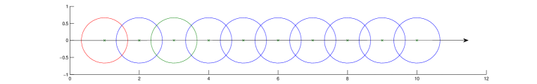
  Figure 1: Packing toy example. The points are at position $1,2,\cdots$, each of them occupies a circle of radius $2/3$. $t$ marks of $i$ is $1-i^{-1}$. The Matérn model only retains $1$ while the $2$-Matérn model retains $1$ and $3$.

  To see this more clearly, let us consider the following toy example (fig.1). There is a sequence of points at the positions $1,2,\cdots$ on $[0,\infty)$. Each point occupies a ball of radius $2/3$ around it. The mark $t$ is assigned to the point at position $i$ is $1-1/i$. Thus, in this setting, the retention mechanism of the Matérn model only retains the point at position $1$ whereas either all points at odd positions or all points at even positions form a contention free set.
  In practice, A. Busson and G. Chelius [9] have conducted a simulation where the contention mechanism described in the above example is used and the Matérn retention mechanism is applied to a Poisson point process. Let $r$ be the radius of the disc occupied by points in the Poisson p.p. Then, for each retained point, the disc of radius $2r$ centered on this point is its blocked area, i.e. no other point can be retained within this area. In the jamming regime, i.e. when the intensity of the proposed Poisson p.p. goes to $\infty$, only $75\%$ of the plane is blocked. As the intensity of the proposed p.p. is very large, one can find a proposed point in the un-blocked area with high probability. This point is not retained by Matérn model although it does not contend with any retained point.
  To alleviate this drawback, we propose the $k$-Matérn models. Let us start with the example of fig.1. The point at position $3$ is prohibited by (i.e. contends with and has smaller $t$ mark than) the point at position $2$, which has already been prohibited by a retained point. Thus, retaining the point at position $3$ can do no harm. Generalizing this, we can retain more points by allowing any point that is not prohibited by any point retained by the Matérn model. This results in the $2$-Matérn model. However, this model also has its own drawback; it is ”over-greedy“ since two points retained by the $2$-Matérn model can still contend with each other. For example, consider the situation in fig. 2. There are five points at five vertices of a pentagon. Any two adjacent vertices contend with each other. The $t(.)$ marks are: $t(A)=.1$, $t(B)=.2$, $t(C)=.4$, $t(D)=.5$ and $t(E)=.3$. Thus, the Matérn model retains vertex $A$, and the $2$-Matérn model retains $A,D$ and $C$ (because D and C do not contend with $A$, which is the only point retained by the Matérn model). However, we can see that $D$ and $C$ contend since they are adjacent.
  

  

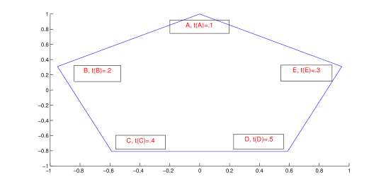
  Figure 2: An example where two points retained by the $2$-Matérn model contend. Five points are placed at the vertices of a pentagon. Two adjacent vertices contend with each other. The $t$ marks are as shown in the figure.

  By iterating the procedure used to obtain the $2$-Matérn model, we can recursively define the $k+1$-Matérn model from the $k$-Matérn model as follows: the subset of points retained by the $k+1$-Matérn model is the proposed points which are not prohibited by any point retained by the $k$-Matérn model. Within this context, the Matérn model is the $1$-Matérn model and the proposed p.p. $\Phi$ is the $0$-Matérn model.
  More formally, the $k$-Matérn model is defined as a dependent thinning of the proposed Poisson p.p. $\Phi$. The contention mechanism is the same as that of the Matérn model. As for the retention mechanism, each proposed point $x$ is assigned a uniform independent random mark $t(x)$ in $[0,1]$ and a sequence of binary marks $e_{0}(x),e_{1}(x),\cdots$. The meaning of this sequence is: ”$x$ is retained by the $k$-Matérn model iff the mark $e_{k}(x)=1$”. In the temporal view-point, at each time $t$ from $0$ to $1$, a fresh Poisson p.p. arrives. Upon arrival, each point $x$ is retained by the $k+1$-Matérn model ($e_{k+1}(x)=1$) iff it finds no arrived contender which is retained by the $k$-Matérn model. In the graph theoretic construction, we construct the conflict graph as for the Matérn model. A point $x$ is assigned the mark $e_{k+1}(x)=1$ if for every child $y$ of $x$ (vertex that has an edge from $x$ to it, we recall that the conflict graph is acyclic so the notion of child is well-defined), we have $e_{k}(y)=0$. Note that $e_{0}(x)=1$ for all $x$ in $\Phi$ by definition.
  Before going to our next packing model, notice that the even-Matérn models are not, strictly speaking, “packing” models. As we have already seen with the $2$-Matérn model, two points retained by an even-Matérn model can still contend with each other, so that the retained subset is not necessarily contention free. In general, the odd-Matérn models retain points in a conservative way while the even-Matérn ones do so in an over-greedy way.
  

• $\infty$-Matérn model: The last model considered in this paper is the one arising in the study of wireless ad hoc networks using the Carrier Sensing Multiple Access (CSMA) protocol [6]. This model is named $\infty$-Matérn model, as we will show in Section 3.2 that it is the “limit” of the $k$-Matérn models when $k$ goes to $\infty$. It is also a “perfect” packing model as its retention mechanism is neither too conservative nor too greedy.
  

  The $\infty$-Matérn model can also be seen as a dependent thinning of the proposed Poisson p.p. $\Phi$. This thinning shares the same contention mechanism as all $k$-Matérn models. The only difference lies in the retention mechanism. At this point, it would be convenient to keep the notation analogous to that of $k$-Matérn models. Each proposed point $x$ is assigned a uniform mark $t(x)$ on $[0,1]$ and a Boolean mark $e_{\infty}(x)$ whose meaning is: “$x$ is retained by the $\infty$-Matérn models iff $e_{\infty}(x)=1$“. Temporally, when the point $x$ arrives at time $t(x)$, it is assigned the mark $e_{\infty}(x)=1$ (retained) iff it finds no contender which has arrived before and has already been assigned mark $1$. If one considers only the p.p. retained by the $\infty$-Matérn model, it falls into a class of processes called Spatial Pure Birth p.p.s, which was suggested by Møller ( see [10], Section 2, paragraph 2). A pure birth process in the plane is a Markovian system of p.p.s indexed by time $t$, or equivalently, a Markov process whose states are p.p.s. At an instant of time, points are ”born”, i.e. added to the existing p.p. where the birth probability only depends on the current configuration $\phi$ of the process. The process is controlled by the birth rate $b$, which is a positive function $b(x,\phi)$ satisfying:

  $$\int_{A}b(x,\phi)dx<\infty,$$

  for any bounded subset $A$ of $\mathbb{R}^{2}$ and any configuration $\phi$. Thus, given that the configuration of the process at time $t$ is $\phi$, the probability that there is a point born in $A$ in the infinitesimal time interval $[t,t+ds]$ is:

  $$ds\int_{A}b(x,\phi)dx+o(ds).$$

  In the $\infty$-Matérn model, assuming that the intensity of the proposed process is $\lambda$, the birthrate can be expressed as:

  $$b(x,\phi)=\lambda\textbf{P}(\textnormal{a point at $x$ does not contend with any point in $\phi$}).$$

  The graph-theoretic definition of the retention mechanism of the $\infty$-Matérn is as follows: a point is retained iff, in the conflict graph, none of its children is retained. This is a recursive definition, the well-definedness of which depends on the structure of the conflict graph. In Section 3.2, we will show that under some mild conditions, the conflict graph of $\Phi$ is such that the previous recursive definition works well.

2 State of the Art

Due to their wide range of applications, random packing models have attracted a lot of attention. The methods employed range from real experiments [11, 12], to simulations [13, 9] and numerical approximations [14, 9].
On the other hand, the vast number of experimental publications here is in sharp contrast with the lack of rigorous mathematical results, especially for dimensions larger than 2. In dimension 1, packing models are more analytically tractable due to the shielding effect, [15]. The first model of this kind is the car parking model which was independently studied by A. Renyi [16] and by A. Robin and H. Dvoretzky [17]. In this model, cars of fixed length are parked in the same manner as in the $\infty$-Matérn model. Consider an observation window $[0,x]$ and let $N(x)$ be the number of cars parked in this window when there is an infinite number of cars to be parked (saturated regime). Rényi showed that $N(x)$ satisfies the law of large number (LLN):

$$\lim_{x\rightarrow\infty}\frac{N(x)}{x}=C\approx 0.74759\qquad\textnormal{a.s.},$$

where $C$ is called the packing density. A. Robin and H. Dvoretzk [17] sharpened this result to a central limit theorem (CLT):

$$\frac{N(x)-Cx}{\sqrt{\rm{var}(N(x))}}\longrightarrow\mathcal{N}(0,1)\qquad\textnormal{ in distribution as }x\rightarrow\infty.$$

Various extensions of the above models were considered like the non-saturated regime (the number of cars to be parked is finite), random car lengths, etc. [18, 19]. The latter is also known under the name random interval packing and has many applications in resource allocation in communication theory. For the above models, the obtained results concern the packing density, LLN, CLT, the distribution of packed intervals and that of vacant intervals.
For dimension more than $1$, in his PhD thesis [7], B. Matérn introduced 3 types of hard-core models. Among these, the Matérn type I model is the simplest. It is constructed as a dependent thinning of a Poisson proposed p.p. Each proposed point has a hard-disk of radius $r$ attached to it. A point is accepted if its attached disk does not overlap with that of any other point. The Matérn type II models have already been discussed in Section 1 and can be seen as an instance of the 1-Matérn model. The Matérn type III model, which Matérn just briefly mentioned, can be seen as a special case of the $\infty$-Matérn model in this paper. Moment measures and correlation functions can be computed for the Matérn type II models. The Matérn type III model proves to be far less tractable. In his work, Matérn asserted:”even an attempt to find the [packing density] tends to rather formidable mathematics“.
At the same time, I. Palasti [20] considered an extension of the car parking problem to the plane, where cars are rectangles of fixed sides. The car parking problem for the $n$ dimensional space is then defined in the same manner. She conjectured that the packing density is $C^{n}$ for the car parking model in $n$ dimensional space. This conjecture was, however, invalidated later by experimental data [21].
One may recognize that the Matérn type III model and the car parking model are just two names of the same object. In fact, this model is most well-known as Random Sequential Absorbtion model (RSA). If we consider the $\infty$-Matérn model defined only in a finite window, then it coincides with the Poisson RSA model. The reader should refer to the paper by H. Solomon and H. Weiner [15] for a review on the progress in the study of the RSA model up to that time.
The most noticable advance in this field is a series of papers by M.D. Penrose, J.E. Yukich and Y. Baryshnikov. Based on a general LLN and CLT for stablizing functionals, the LLN and CLT were established for the $n$ dimensional RSA model in the non-saturated [22] regime. Y. Baryshnikov and J. E. Yukich [23] later strengthened the above results by proving that, in the thermodynamic limit, the spatial distribution of the p.p. induced by the RSA model converges to that of a Gaussian field after a suitable rescaling in the non-saturated regime. The LLN and CLT for the $n$ dimensional RSA model under saturated regime is proven by T. Schreiber et al [24].
It is worth noting here the difference between our approach and that of the works listed above. As expained earlier in Section 1, in the $\infty$-Matérn model (which also admits the RSA model as a special case), there is a time dimension, along which new points arrive to be packed. We are interested in the dynamic of the induced p.p.s as time passes and more points arrive. In contrast, time is fixed in the aforementioned works. The above authors consider the distribution of the points packed in an observed window and how it converges when the observed window grows to the whole space.

3 The Packing Models

Throughout this paper, every p.p. is equipped with independent and identically distributed (i.i.d.) marks which we call timers. These timers are uniformly distributed on $[0,1]$. The timer of point $x$ is denoted by $t(x)$.
Let us begin with a preliminary transformation that will be used frequently. For each p.p. $\Phi$, we define:

$$T_{A}(\Phi)=\left\{x\in\Phi\ \textnormal{ s.t. }\ t(x)\in A\right\},$$ (1)

for all measurable subsets $A$ of $\mathbb{R}^{+}$. This is the timer based thinning of $\Phi$ in $A$.
The contentions of the points are encoded in the Boolean random field $C$. The meaning of $C$ is that two points $x,y$ contend iff $C(x,y)=1$. Let $\textbf{P}(C(x,y)=1)=h(x,y)$. The assumptions on $C$ are:

$$C(x,y)=C(y,x)\ \forall x,y,\ \textnormal{(symmetry)};$$

$$C(x,y)\textnormal{ are independent r.v.s for unordered pairs }(x,y);$$

$$h(x,y)=h(0,y-x)\textnormal{ }\forall x,y\textnormal{ (translation invariance)}.$$

Note that the contention field is defined independently of the timers. If $C(x,y)=1$ then $x$ and $y$ contend with each other regardless of their timers.

3.1 Packing Models by Thinning

In this subsection, we define the Matérn model, the $k$-Matérn model and the $\infty$-Matérn model as thinning transformations of another p.p.. These thinning transformations can be obtained by iteratively applying the following transformation $\Psi$:

$$\Psi(\Phi_{1},\Phi_{2},C)=\{x\in\Phi_{1}\textnormal{ s.t. }\prod_{y\in T_{[0,t(x))}(\Phi_{2})}(1-C(x,y))=1\}.$$

• Matérn model: the Matérn model $M^{1}(\Phi,C)$ of $\Phi$ and of the contention field $C$, is obtained from the thinning transformation

  $$M^{1}(\Phi,C):=\Psi(\Phi,\Phi,C).$$ (2)

  That is:

  $$M^{1}(\Phi,C)=\{x\in\Phi\textnormal{ s.t. }e_{1}(x)=1\},$$ (3)

  where the thinning indicators $e_{1}(x)$ are defined by:

  $$e_{1}(x)=\prod_{y\in T_{[0,t(x))}(\Phi)}(1-C(x,y)).$$ (4)

• $k$-Matérn model: the $k$-Matérn models $M^{k}(\Phi,C)$ of $\Phi$ and $C$ can be recursively defined as

  $$M^{k}(\Phi,C)=\Psi(\Phi,M^{k-1}(\Phi,C),C).$$ (5)

  One can also define the thinning indicator of the $k$-Matérn model and write:

  $$M^{k}(\Phi,C) = \{x\in\Phi\textnormal{ s.t. }e_{k}(x)=1\},$$ (6)

  with

  $$e_{k}(x) = \prod_{y\in T_{[0,t(x))}(M^{k-1}(\Phi,C))}(1-C(x,y))$$ (7)

  $$= \prod_{y\in T_{[0,t(x))}(\Phi)}(1-e_{k-1}(y)C(x,y)).$$

• $\infty$-Matérn model: the $\infty$-Matérn model $M^{\infty}(\Phi,C)$ of $\Phi$ and $C$ can be defined as:

  $$M^{\infty}(\Phi,C)=\Psi(\Phi,M^{\infty}(\Phi,C),C),$$ (8)

  in a sense to be made clear in the next subsection. An equivalent expression is:

  $$M^{\infty}(\Phi,C)=\{x\in\Phi\textnormal{ s.t. }e_{\infty}(x)=1\},$$ (9)

  with $e_{\infty}$ satisfying the fixed point equation

  $$e_{\infty}(x) = \prod_{y\in T_{[0,t(x))}(M^{\infty}(\Phi,C))}(1-C(x,y))$$ (10)

  $$= \prod_{y\in T_{[0,t(x))}(\Phi)}(1-e_{\infty}(y)C(x,y)).$$

In the above definitions, we adopt the convention that the product over an empty set is $1$.

3.2 The $\infty$-Matérn Model is Well Defined

In this subsection, we give a sufficient condition for the $\infty$-Matérn model to be well-defined. We then prove that the $\infty$-Matérn model is the limit of the $k$-Matérn models in the sense that:

$$\forall x\in\Phi\qquad e_{\infty}(x)=\lim_{k\rightarrow\infty}e_{k}(x)\textnormal{ a.s. }$$

3.2.1 Conflict Graph

Here we formally define the notion of conflict graph which will play a central role in the forthcoming proofs. Given a p.p. $\Phi$ and a contention field $C$, the associated conflict graph is the directed graph $G(\Phi,C)=(\Phi,\mathcal{E}(\Phi))$, where $\mathcal{E}(\Phi)=\{(x,y)\in\Phi^{2}$ s.t. $t(y)<t(x),C(x,y)=1\}$. That is, we put an edge from $x$ to $y$ iff $x$ and $y$ contend and the timer of $x$ is larger than that of $y$. It is easy to check that $G(\Phi,C)$ is acyclic.
We now introduce the notion of conflict indicator function of a graph. To this end we consider an arbitrary acyclic directed graph $H$ and a vertex $o$ in it. Let $K^{*}_{H}(o)$ be the positive connected component of $o$, i.e. the set of points $x$ such that there is a directed path in $H$ from $o$ to $x$. For all positive integer $n$, let $K^{n}_{H}(o)$ be the $n$-step positive connected component of $o$, i.e. the set of points $x$ such that there is a path of length at most $n$ from $o$ to $x$. Note that $o$ is always contained in $K^{*}_{H}(o)$ and $K^{n}_{H}(o)$ by convention. We say that $H$ has no infinite positive percolation if we have $|K^{*}_{H}(x)|<\infty$ for all $x$ in $\Phi$.

In the following, by abuse of notation, we use the same notation for a set of vertices and the subgraph induced by this set. The conflict indicator function $e(H,o)$, which takes value in $\{0,1\}$, is recursively defined as:

$$e(H,o):=\left\{\begin{array}[]{l r }1&\textnormal{ if }H=(\{o\},\emptyset)\\ \prod_{(o,x)\in H}(1-e(K^{*}_{H}(x),x))&\textnormal{otherwise.}\end{array}\right.$$ (13)

One can easily see that when $|K^{*}_{H}(o)|<\infty$, $e(H,o)$ is well-defined and equal to $e(K^{*}_{H}(o),o)$. We will need the following lemmas in which we assume that the condition

$$\int_{\mathbb{R}^{2}}h(0,x)dx=N<\infty$$ (14)

is satisfied:

Lemma 1

For an homogeneous Poisson p.p. $\Phi$ of intensity $\lambda<N^{-1}$, the conflict graph $G(\Phi,C)$ has no infinite positive percolation a.s.

Proof.
For this proof we introduce the notion of infinite percolation. In $G(\Phi,C)$, we remove the direction of the edges and let $S(x)$ be the connected component of the resulting graph containing $x$. We say that the graph $G(\Phi,C)$ has no infinite percolation if $|S(x)|<\infty$ for all $x$. Clearly, if $G(\Phi,C)$ has no infinite percolation then it has no infinite positive percolation. We now show that $G(\Phi,C)$ has no infinite percolation a.s. For each $x$:

$$\textbf{E}[|S(x)|]\leq 1+\sum_{n=1}^{\infty}\textbf{E}\left[\sum_{y\in\Phi}\textbf{1}_{\textnormal{there is a path of length $n$ from $x$ to $y$}}\right]$$

$$\leq 1+\sum_{n=1}^{\infty}\textbf{E}\left[\textnormal{number of non self-intersecting paths of length $n$ starting from $x$}\right]$$

$$=1+\sum_{n=1}^{\infty}\textbf{E}\left[\sum_{y_{1},y_{2},\cdots,y_{n}\textnormal{pairwise different}\in\Phi}\textbf{1}_{C(x,y_{1})=1,C(y_{1},y_{2})=1,\cdots,C(y_{n-1},y_{n})=1}\right].$$

Using the independence of $C(x,y_{1}),C(y_{1},y_{2}),\cdots,C(y_{n-1},y_{n})$ and the reduced Campbell formula we have:

$$\sum_{i=1}^{n}\textbf{E}\left[\sum_{y_{1},y_{2},\cdots,y_{n}\textnormal{pairwise different}\in\Phi}\textbf{1}_{C(x,y_{1})=1,C(y_{1},y_{2})=1,\cdots,C(y_{n-1},y_{n})=1}\right]$$

$$=\sum_{i=1}^{n}\int_{(\mathbb{R}^{2})^{n}}h(x,y_{1})h(y_{1},y_{2})\cdots h(y_{n-1},y_{n})\Lambda^{(n!)}(dy_{1},dy_{2},..dy_{n}),$$

where $\Lambda^{(n!)}$ is the $n^{th}$ factorial moment measure of $\Phi$. This measure is known to be $\lambda^{n}l$, where $l$ denotes the Lebesgue measure on $\mathbb{R}^{2}$. Thus, using the fact that $h$ is translation invariant, we can change the variables from $y_{i}$ to $y_{i}-y_{i-1}$ and $y^{1}$ to $y^{1}-x$ to get:

$$\textbf{E}[|S(x)|]$$

$$\leq 1+\sum_{n=1}^{\infty}\int_{(\mathbb{R}^{2})^{n}}h(0,y_{1}-x)h(0,y_{2}-y_{1})\cdots h(0,y_{n}-y_{n-1})\lambda^{n}dy_{1}dy_{2}\cdots dy_{n}$$

$$=1+\sum_{n=1}^{\infty}\int_{(\mathbb{R}^{2})^{n}}h(0,y_{1})h(0,y_{2})\cdots h(0,y_{n})\lambda^{n}dy^{1}dy^{2}\cdots dy^{n}$$

$$=1+\sum_{n=1}^{\infty}\lambda^{n}N^{n}=(1-\lambda N)^{-1}<\infty.$$

Thus $|S(x)|<\infty$ a.s. and this proves the lemma.

$\Box$

Lemma 2

If $G(\Phi,C)$ has no infinite positive percolation, then for all $x\in\mathbb{R}^{2}$, $G(\Phi\cup\{x\}^{+},C)$ has no infinite positive percolation either. The $+$ superscript means that the timer for the additional point is set to $1$.

Proof.
Note that since (14) is satisfied, any point $x$ in the plane has only a finite number of contenders in $\Phi$ a.s.. Thus, by adding a point to $\Phi$ and letting the timer of this point be $1$, we can only add a finite number of edges to the conflict graph. These edges are the edges connecting the added point to its contenders in $\Phi$. So, if $G(\Phi,C)$ has no infinite positive percolation, then $G(\Phi\cup\{x\}^{+},C)$ has no infinite positive percolation neither.

$\Box$

Lemma 3

For an homogeneous Poisson p.p. $\Phi$ of intensity $\lambda<\infty$, the conflict graph $G(\Phi,C)$ has no infinite positive percolation.

Proof.
We prove this lemma by induction on the intensity of $\Phi$. Fix a positive $\lambda_{0}<N^{-1}$. If $\lambda<\lambda_{0}$, then $G(\Phi,C)$ does not have infinite positive percolation thanks to Lemma 1. Now let $n$ be a positive integer and suppose that $G(\Phi,C)$ does not have infinite positive percolation for any homogeneous Poisson p.p. $\Phi$ with intensity smaller than $n\lambda_{0}$. Consider an homogeneous Poisson p.p. $\Phi$ with intensity $\lambda$ such that $n\lambda_{0}\leq\lambda<(n+1)\lambda_{0}$. Since $T_{[\frac{n\lambda_{0}}{\lambda},1]}(\Phi)$ is an homogeneous Poisson p.p. with intensity $\lambda-n\lambda_{0}\leq\lambda_{0}$, $G(T_{[\frac{n\lambda_{0}}{\lambda},1]}(\Phi),C)$ has no infinite percolation by Lemma 1.
Consider a point $x$ in $\Phi$. If $t(x)<\frac{n\lambda_{0}}{\lambda}$, then $K^{*}_{G(\Phi,C)}(x)=K^{*}_{G(T_{[0,t(x))}(\Phi),C)}(x)$ is finite by the fact that $T_{[0,t(x))}(\Phi)$ is an homogeneous Poisson p.p. of intensity smaller than $n\lambda^{0}$ and the induction hypothesis. If $t(x)\geq\frac{n\lambda_{0}}{\lambda}$, we rewrite $K^{*}_{G(\Phi,C)}(x)$ as:

$$K^{*}_{G\left(T_{[\frac{n\lambda_{0}}{\lambda},1]}(\Phi),C\right)}(x)\bigcup\left(\bigcup_{y\in K^{*}_{G\left(T_{[\frac{n\lambda_{0}}{\lambda},1]}(\Phi),C\right)}(x)}K^{*}_{G\left(T_{[0,\frac{n\lambda_{0}}{\lambda})}(\Phi)\cup\left(y\right)^{+},C\right)}(y)\right).$$

The first term is the set of points accessible from $x$ with timer larger than $\frac{n\lambda_{0}}{\lambda}$; the second term is the set of points accessible from $x$ with timer smaller than $\frac{n\lambda_{0}}{\lambda}$. The second term can in turn be decomposed as the union of the sets of points accessible from $y$ with timer smaller than $\frac{n\lambda_{0}}{\lambda}$, for all $y$ accessible form $x$ with timer larger than $\frac{n\lambda_{0}}{\lambda}$. Since $G\left(T_{[\frac{n\lambda_{0}}{\lambda},1]}(\Phi),C\right)$ has no infinite positive percolation, we have that the first term is finite and the union in the second term is a finite union. Moreover, by Lemma 2 and the induction hypothesis, we have that each term in this finite union is finite. Thus $K^{*}_{G(\Phi,C)}(x)$ is finite, which terminates the proof.

$\Box$

3.2.2 Sufficient Condition

Let us first state the main result:

Proposition 1

If the contention field $C$ satisfies (14), then the $\infty$-Matérn model of the Poisson point process is well-defined in the sense that its thinning indicator $e_{\infty}(.)$ is well defined.

The proof of this proposition is based on the following lemma:

Lemma 4

For all p.p.s $\Phi$ such that $G(\Phi,C)$ has no infinite positive percolation, we have $e_{\infty}(x)=e(K^{*}_{G(\Phi,C)}(x),x)$, where $e(.)$ is the thinning indicator function defined in (13). This is also the only solution of Equation (10).

Proof. Since $G(\Phi,C)$ has no infinite positive percolation, $e(K^{*}_{G(\Phi,C)}(x),x)$ is well defined for all $x$. As $K^{*}_{G(\Phi,C)}(x)=x\cup\left(\bigcup_{y\textnormal{ s.t. }(x,y)\in G(\Phi,C)}K^{*}_{G(\Phi,C)}(y)\right),$ we have that $e(K^{*}_{G(\Phi,C)}(x),x)$ satisfies Equation (10) by definition.
For uniqueness, let $e(x)$ be a solution of (10). We prove by induction on the size of $K^{*}_{G(\Phi,C)}(x)$ that $e(x)=e(K^{*}_{G(\Phi,C)}(x),x)$.
For any $x$ such that $|K^{*}_{G(\Phi,C)}(x)|=1$, we have $K^{*}_{G(\Phi,C)}(x)=\{x\}$ or equivalently, $x$ has out degree $0$ in the conflict graph. Hence

$$e(x)=e(K^{*}_{G(\Phi,C)}(x),x)=1.$$

Note that such $x$ always exists by the assumption that $G(\Phi,C)$ has no infinite percolation.
Suppose that for all $y$ such that $|K^{*}_{G(\Phi,C)}(y)|<n$, we have $e(y)=e(K^{*}_{G(\Phi,C)}$ $(y),y)$. Let us consider an $x$ such that

$$|K^{*}_{G(\Phi,C)}(x)|=n$$

(if there are any). For $y$ such that $(x,y)\in G(\Phi,C)$, we have $|K^{*}_{G(\Phi,C)}(y)|<n$. Thus, $e(y)=e(K^{*}_{G(\Phi,C)}(y),y)$. Then:

$$e(x) =\prod_{y\in T_{[0,t(x))}(\Phi)}(1-e(y)C(x,y))=\prod_{y\in\Phi\textnormal{ s.t. }t(y)<t(x)}(1-e(y)C(x,y))$$

$$=\prod_{y\in\Phi\textnormal{ s.t. }t(y)<t(x),C(x,y)=1}(1-e(y))=\prod_{y\in\Phi\textnormal{ s.t. }(x,y)\in G(\Phi,C)}(1-e(y))$$

$$=\prod_{y\in\Phi\textnormal{ s.t. }(x,y)\in G(\Phi,C)}(1-e(K^{*}_{G(\Phi,C)}(y),y))=e(K^{*}_{G(\Phi,C)}(x),x).$$

Thus, for all $x$ such that $|K^{*}_{G(\Phi,C)}(x)|<n+1$ we have

$$e(x)=e(K^{*}_{G(\Phi,C)}(x),x).$$

This completes the proof of uniqueness.

$\Box$

Now, it is straightforward to see that when (14) is satisfied, the conflict graph associated with $\Phi$ has no infinite positive percolation (Lemma 3). Thus, the $\infty$-Matérn thinning indicators are well-defined (Lemma 4) and are the only solution of (10). Note that the arguments in the above proof can be extended to the case where $\Phi$ is inhomogeneous to obtain the following proposition.

Proposition 2

Let $\Phi$ be an inhomogeneous Poisson p.p. of intensity measure $\Lambda$. If we have:

$$\sup_{x\in\mathbb{R}^{2}}\int_{\mathbb{R}^{2}}h(x,y)d\Lambda(y)=\mathcal{N}<\infty,$$ (15)

then the $\infty$-Matérn model is well-defined in the sense that its thinning indicators $e_{\infty}(x)$ are well defined.

3.2.3 The $\infty$-Matérn Model as Limit of the $k$-Matérn Models

In this part we explain the meaning of the subscript $\infty$ in the definition of the $\infty$-Matérn model. More precisely, we prove that if the conflict graph has no infinite positive percolation, then the thinnning indicators are such that:

$$\forall x\in\Phi\qquad e_{\infty}(x)=\lim_{k\rightarrow\infty}e_{k}(x)\textnormal{ a.s. }$$

Recall that $e(.)$ is the thinning indicator function defined in (13) and $K^{k}(x)$ is the $k$-step positive connected component of $x$. Let us begin with an important result relating the thinning indicators of the $k$-Matérn model with the conflict indicators.

Proposition 3

For all $k\in\mathbb{N}$: $e_{k}(x)=e(K^{k}_{G(\Phi,C)}(x),x)$.

Proof
We prove this by induction. The base case $k=0$ is trivial since $e_{0}(x)=e(K^{0}_{G(\Phi,C)}(x),x)=1.$ For $k\geq 1$ we have by definition:

$$e_{k}(x) =\prod_{y\in T_{[0,t(x))}(\Phi)}(1-e_{k-1}(y)C(x,y))$$

$$=\prod_{y\in\Phi\textnormal{ s.t. }t(y)<t(x),C(x,y)=1}(1-e_{k-1}(y))$$

$$=\prod_{y\in\Phi\textnormal{ s.t. }(x,y)\in G(\Phi,C)}(1-e_{k-1}(y)).$$

Now, $e_{k-1}(y)=e(K^{k-1}_{G(\Phi,C)}(y),y)$ by induction hypothesis. We have:

$$e_{k}(x)=\prod_{y\in\Phi\textnormal{ s.t. }(x,y)\in G(\Phi,C)}(1-e(K^{k-1}_{G(\Phi,C)}(y),y))=e(K^{k}_{G(\Phi,C)}(x),x).$$

$\Box$

Proposition 4

If the conflict graph $G(\Phi,C)$ has no infinite positive percolation, then:

$$\forall x\in\Phi\qquad e_{\infty}(x)=\lim_{k\rightarrow\infty}e_{k}(x)\textnormal{ a.s. }$$

Proof
If the conflict graph has no infinite positive percolation, then $K^{*}_{G(\Phi,C)}(x)$ is finite and $K^{*}_{G(\Phi,C)}(x)=K^{|K^{*}_{G(\Phi,C)}(x)|}_{G(\Phi,C)}(x)$ for all $x$. It then follows from Lemma 4 and Proposition 3 that the sequence $e_{k}(x)$ is constant for $k>|K^{*}_{G(\Phi,C)}(x)|$ and this constant is equal to $e_{\infty}(x)$.

$\Box$

4 The Generating Functional

4.1 Some Background

For a p.p. $\Xi$, for all functions $v$ from $\mathbb{R}^{2}$ to $\mathbb{R}^{+}$ satisfying:

$$\textbf{E}\left[\sum_{x\in\Xi}|1-v(x)|\right]<\infty,$$ (16)

we have $\sum_{x\in\Xi}|1-v(x)|<\infty$ a.s. Since $|\log(t)|<|1-t|$ for all $t>0$, we have that $\sum_{x\in\Xi}|\log(v(x))|<\infty$ a.s.. Hence the sum $\sum_{x\in\Xi}\log(v(x))$ is well-defined a.s. and is itself a random variable. Thus, we can define:

$$G_{\Xi}(v)=\textbf{E}\left[\prod_{x\in\Xi}v(x)\right]=\textbf{E}\left[\exp\left(\sum_{x\in\Xi}\log(v(x))\right)\right],$$

as the generating functional of $\Xi$. It encodes all the information about the distribution of $\Xi$. Many properties of $\Xi$ such as the void probability, the contact distribution, the laplace transform of its Shot-Noise process can be computed in terms of its generating functional (see [25, 26]).
In this section we are interested in the generating functionals $G_{M^{k}(\Phi,C)}(v(.))$, where $\Phi$ is a Poisson p.p. of intensity measure $\Lambda$ and $v$ is a function from $\mathbb{R}^{2}$ to $[0,1]$ such that:

$$\int_{\mathbb{R}^{2}}|1-v(x)|\Lambda(dx)<\infty.$$ (17)

Remark:

• The condition (17) is equivalent to $\textbf{E}[\sum_{x\in\Phi}|1-v(x)|]<\infty$ (Campbell’s formula). Thus, this condition guarantees that the generating functional of $\Phi$ is well-defined at $v$. Since $M^{k}(\Phi,C)$ is dominated by $\Phi$, the generating functional of $M^{k}(\Phi,C)$ is also well-defined at $v$.

• Although there are functions $v$ such that the generating functional of $M^{k}(\Phi,C)$ is well-defined at $v$ while the generating functional of $\Phi$ is not, we will not consider this case here for two reasons:

  • All informations about the distribution of a p.p. are encoded in the generating functional with $v$ having bounded support. These functions $v$ satisfy (17) automatically.

  • As we will see later, this condition guarantees nice convergence properties.

In order to study the functionals $G_{M^{k}(\Phi,C)}(v(.))$, it will be useful to extend our model to the case where the timers are no longer restricted to $[0,1]$ and take values “uniformly” on $\mathbb{R}^{+}$. This makes our p.p. $\Phi$ no longer a marked Poisson p.p. but a Poisson p.p. on $\mathbb{R}^{2}\times\mathbb{R}^{+}$, with the last dimension being the timer. The intensity measure of $\Phi$ satisfies $\textbf{E}[\Phi(A\times[0,t])]=t\Lambda(A),$ for all Borel sets $A$ and all positive real numbers $t$. The description of the timer based thinning and the $\Psi$ thinning are kept unchanged. Our aim is to study the following functionals:

$$f_{k,\Lambda}(t,v):=G_{M^{k}(T_{[0,t)}(\Phi),C)}(v(.)).$$ (18)

The link between the model with timers restricted to $[0,1]$ and the last model is that the generating functional of the former is $f_{k,\Lambda}(1,v)$.

In this section, we gather our major results regarding the evolution over time $t$ of the $f_{k,\Lambda}(t,v)$ functional. More precisely, we prove that it is the solution of some differential equation w.r.t. $t$. First we show that it is continuous.

Proposition 5

For all $k$ and all $v$ satisfying the condition (17), $f_{k,\Lambda}(t,v)$ is continuous in $t$.

Proof. For all $t_{1}<t_{2}$ and all $k\in\mathbb{N}$:

$$T_{[0,t_{1})}(M^{k}(T_{[0,t_{2})}(\Phi),C))=M^{k}(T_{[0,t_{1})}(\Phi),C).$$

Thus, for all $t$ positive and $\epsilon$ positive:

$$f_{k,\Lambda}(t+\epsilon,v)$$

$$=\textbf{E}\left[\prod_{x\in M^{k}(T_{[0,t+\epsilon)}(\Phi),C)}v(x)\right]$$

$$=\textbf{E}\left[\prod_{x\in T_{[0,t)}(M^{k}(T_{[0,t+\epsilon)}(\Phi),C))}v(x)\prod_{x\in T_{[t,t+\epsilon)}(M^{k}(T_{[0,t+\epsilon)}(\Phi),C))}v(x)\right]$$

$$=\textbf{E}\left[\prod_{x\in M^{k}(T_{[0,t)}(\Phi),C)}v(x)\prod_{x\in T_{[t,t+\epsilon)}(M^{k}(T_{[0,t+\epsilon)}(\Phi),C))}v(x)\right].$$

Since $M^{k}(T_{[0,t+\epsilon)}(\Phi),C)$ is dominated by $T_{[0,t+\epsilon)}(\Phi)$, $T_{[t,t+\epsilon)}(M^{k}(T_{[0,t+\epsilon)}(\Phi),C))$ is dominated by $T_{[t,t+\epsilon)}(T_{[0,t+\epsilon)}(\Phi))=T_{[t,t+\epsilon)}(\Phi)$. Let $v_{+}(x)=\max\{1,v(x)\}$ and $v_{-}(x)=\min\{1,v(x)\}$, we have a.s.

$$\prod_{x\in T_{[t,t+\epsilon)}(\Phi)}v_{+}(x)\geq\prod_{x\in T_{[t,t+\epsilon)}(M^{k}(T_{[0,t+\epsilon)}(\Phi),C))}v_{+}(x)$$

$$\geq\prod_{x\in T_{[t,t+\epsilon)}(M^{k}(T_{[0,t+\epsilon)}(\Phi),C))}v(x)$$

$$\geq\prod_{x\in T_{[t,t+\epsilon)}(M^{k}(T_{[0,t+\epsilon)}(\Phi),C))}v_{-}(x)\geq\prod_{x\in T_{[t,t+\epsilon)}(\Phi)}v_{-}(x).$$

Thus:

$$f_{k,\Lambda}(t,v)\exp\{\epsilon\int_{\mathbb{R}^{2}}|1-v(x)|\Lambda(dx)\}\geq f_{k,\Lambda}(t,v)\exp\{\epsilon\int_{\mathbb{R}^{2}}(v_{+}(x)-1\Lambda(dx)\}$$

$$=\textbf{E}\left[\prod_{x\in M^{k}(T_{[0,t)}(\Phi),C)}v(x)\prod_{x\in T_{[t,t+\epsilon)}(\Phi)}v_{+}(x)\right]\geq\textbf{E}\left[\prod_{x\in M^{k}(T_{[0,t+\epsilon)}(\Phi),C)}v(x)\right]$$

$$=f_{k,\Lambda}(t+\epsilon,v)\geq\textbf{E}\left[\prod_{x\in M^{k}(T_{[0,t)}(\Phi),C)}v(x)\prod_{x\in T_{[t,t+\epsilon)}(\Phi)}v(x)\right]$$

$$=\textbf{E}\left[\prod_{x\in M^{k}(T_{[0,t)}(\Phi),C)}v(x)\prod_{x\in T_{[t,t+\epsilon)}(\Phi)}v_{-}(x)\right]$$

$$=f_{k,\Lambda}(t,v)\exp\left\{-\epsilon\int_{\mathbb{R}^{2}}(1-v_{-}(x))\Lambda(dx)\right\}$$

$$\geq f_{k,\Lambda}(t,v)\exp\left\{-\epsilon\int_{\mathbb{R}^{2}}|1-v(x)|\Lambda(dx)\right\}.$$

Doing the same, we have:

$$f_{k,\Lambda}(t-\epsilon,v)\exp\{\epsilon\int_{\mathbb{R}^{2}}|1-v(x)|\Lambda(dx)\}\geq f_{k,\Lambda}(t,v)$$

$$\geq f_{k,\Lambda}(t-\epsilon,v)\exp\left\{-\epsilon\int_{\mathbb{R}^{2}}|1-v(x)|\Lambda(dx)\right\}.$$

Letting $\epsilon$ go to $0$ completes our proof.

$\Box$.

4.2 Differential Equation for the $\infty$-Matérn Model

Let $H$ be the map that associates to a function $v$ from ${\mathbb{R}^{2}}\to[0,1]$ and a point $x\in\mathbb{R}^{2}$ the function

$$H(v,x)(y)=v(y)(1-h(x,y)).$$ (19)

It is easy to see that $H(v,x)(.)$ is a function from ${\mathbb{R}^{2}}$ to $[0,1]$.

Theorem 1

For any locally finite measure $\Lambda$, the functional $f_{\infty,\Lambda}$ satisfies the following equation:

$$f_{\infty,\Lambda}(0,v(.)) = 1$$ (20)

$$\frac{df_{\infty,\Lambda}(t,v(.))}{dt} = -\int_{\mathbb{R}^{2}}f_{\infty,\Lambda}(t,H(v,x))(1-v(x))\Lambda(dx).$$

The main idea behind this theorem is to divide the p.p. $\Phi$ into thin layers $T_{[t,t+\epsilon)}(\Phi)$ such that the points in each layer are so sparse that the effect of contention is negligible. Then, one can consider the retained p.p.s in these layers as Poisson p.p.s
In particular, we need to prove that:

$$\lim_{\epsilon\rightarrow 0}\frac{f(t+\epsilon,v)-f(t,v)}{\epsilon}=-\int_{\mathbb{R}^{2}}f(t,H(v,x))(1-v(x))\Lambda(dx)$$ (21)

$$\lim_{\epsilon\rightarrow 0}\frac{f(t,v)-f(t-\epsilon,v)}{\epsilon}=-\int\limits_{\mathbb{R}^{2}}f(t,H(v,x))(1-v(x))\Lambda(dx),$$ (22)

for any locally finite $\Lambda$. We will need the following lemmas:

Lemma 5

For any p.p. $\Xi$ and any function $v$ taking value in $\mathbb{R}^{+}$ such that:

$$\textbf{E}\left[\sum_{x\in\Xi}|1-v(X)|\right]<\infty,$$

we have:

$$\prod_{x\in\Xi}v(x)=1+\sum_{i=1}^{\infty}(-1)^{i}\sum_{(x_{1},\cdots,x_{i})\in\Xi^{i!}}\prod_{j=1}^{i}(1-v(x_{j}))\textnormal{ a.s.},$$ (23)

where $\Xi^{i!}$ is the set of unordered $i$-tuples of points in $\Xi$.

Proof. By the same argument as those at the beginning of the section, we have $\prod_{x\in\Xi}v(x)=\exp\{\sum_{x\in\Xi}\log(v(x))\}$ is well-defined and a.s. finite.
Now, to prove that the series in the right hand side of (23) converges, it is enough to show that:

$$1+\sum_{i=1}^{\infty}\sum_{(x_{1},\cdots,x_{i})\in\Xi^{i!}}\prod_{j=1}^{i}|1-v(x_{j})|<\infty\textnormal{ a.s.}.$$

Note that:

$$\sum_{(x_{1},\cdots,x_{i})\in\Xi^{i!}}\prod_{j=1}^{i}|1-v(x_{j})|=\frac{1}{i!}\sum_{x_{1},\cdots,x_{i}\textnormal{ mutually different}\in\Xi}\textnormal{ }\prod_{j=1}^{i}|1-v(x_{j})|$$

$$\leq\frac{1}{i!}\left(\sum_{x\in\Xi}|1-v(x)|\right)^{i}.$$

Hence:

$$1+\sum_{i=1}^{\infty}\sum_{(x_{1},\cdots,x_{i})\in\Xi^{i!}}\prod_{j=1}^{i}|1-v(x_{j})|\leq 1+\sum_{i=1}^{\infty}\frac{1}{i!}\left(\sum_{x\in\Xi}|1-v(x)|\right)^{i}$$

$$=e^{\left(\sum_{x\in\Xi}|1-v(x)|\right)}<\infty.$$

Now the equality can be obtained by writing:

$$\prod_{x\in\Xi}v(x)=\prod_{x\in\Xi}(1-(1-v(x))).$$

$\Box$

Lemma 6

For any $k$, including $\infty$ and any locally finite measure $\Lambda$, we have:

$$\int_{\mathbb{R}^{2}}\textbf{1}_{v(x)<1}(1-v(x))\Lambda(dx)+\int_{\mathbb{R}^{2}}\textbf{1}_{v(x)\geq 1}(1-v(x))e^{-\epsilon\int_{\mathbb{R}^{2}}(1-h(x,y))\Lambda(dy)}\Lambda(dx)$$

$$+\frac{e^{\epsilon\int_{\mathbb{R}^{2}}|1-v(x)|\Lambda(dx)}-1-\epsilon\int_{\mathbb{R}^{2}}|1-v(x)|\Lambda(dx)}{\epsilon}\geq\frac{1-f_{k,\Lambda}(\epsilon,v)}{\epsilon}$$

$$\geq\int_{\mathbb{R}^{2}}\textbf{1}_{v(x)>1}(1-v(x))\Lambda(dx)+\int_{\mathbb{R}^{2}}\textbf{1}_{v(x)\leq 1}(1-v(x))e^{-\epsilon\int_{\mathbb{R}^{2}}(1-h(x,y))\Lambda(dy)}\Lambda(dx)$$

$$-\frac{e^{\epsilon\int_{\mathbb{R}^{2}}|1-v(x)|\Lambda(dx)}-1-\epsilon\int_{\mathbb{R}^{2}}|1-v(x)|\Lambda(dx)}{\epsilon}.$$

In particular:

$$\lim_{\epsilon\rightarrow 0}\frac{f_{k,\Lambda}(\epsilon,v)-1}{\epsilon}=-\int_{\mathbb{R}^{2}}(1-v(x))\Lambda(dx).$$ (24)

Proof. We first use Lemma 5 with $M^{k}(T_{[0,\epsilon)}(\Phi),C)$ in place of $\Xi$ to get:

$$1-f_{k,\Lambda}(\epsilon,v)=\sum_{i=1}^{\infty}(-1)^{i+1}\textbf{E}\left[\sum_{(x_{1},\cdots,x_{i})\in M^{k}(T_{[0,\epsilon)}(\Phi),C)^{i!}}\prod_{j=1}^{i}(1-v(x_{j}))\right]$$

For any $i>1$, we have:

$$\left|\textbf{E}\left[\sum_{(x_{1},\cdots,x_{i})\in M^{k}(T_{[0,\epsilon)}(\Phi),C)^{i!}}\prod_{j=1}^{i}(1-v(x_{j}))\right]\right|$$

$$=\frac{1}{i!}\left|\textbf{E}\left[\sum_{x_{1},\cdots,x_{i}\textnormal{ mutually different}\in M^{k}(T_{[0,\epsilon)}(\Phi),C)^{i!}}\prod_{j=1}^{i}(1-v(x_{j}))\right]\right|$$

$$=\frac{1}{i!}\int_{(\mathbb{R}^{2})^{i}}\prod_{j=1}^{i}\left|1-v(x_{j})\right|m^{i}_{k,\Lambda}(dx_{1},\cdots,dx_{j}),$$

where $m^{i}_{k,\Lambda}$ is the $i$-factorial moment measure of $M^{k}(T_{[0,\epsilon)}(\Phi),C)$. Now, by the fact that $M^{k}(T_{[0,\epsilon)}(\Phi),C)$ is dominated by $T_{[0,\epsilon)}(\Phi)$, its $i$-factorial moment measure is dominated by that of $T_{[0,\epsilon)}(\Phi)$, which is known to be $\epsilon^{i}\prod_{j=1}^{i}\Lambda(dx_{j})$. Thus,

$$\left|\textbf{E}\left[\sum_{(x_{1},\cdots,x_{i})\in M^{k}(T_{[0,\epsilon)}(\Phi),C)^{i!}}\prod_{j=1}^{i}(1-v(x_{j}))\right]\right|$$

$$\leq\frac{1}{i!}\epsilon^{i}\int_{(\mathbb{R}^{2})^{i}}\prod_{j=1}^{i}\left|1-v(x_{j})\right|\prod_{j=1}^{i}\Lambda(dx_{j})=\frac{1}{i!}\epsilon^{i}\left(\int_{\mathbb{R}^{2}}|1-v(x)|\Lambda(dx)\right)^{i}.$$

Hence:

$$-\frac{e^{\epsilon\int_{\mathbb{R}^{2}}|1-v(x)|\lambda(dx)}-1-\epsilon\int_{\mathbb{R}^{2}}|1-v(x)|\lambda(dx)}{\epsilon}=-\sum_{i=2}^{\infty}\frac{1}{i!}\epsilon^{i}\left(\int_{\mathbb{R}^{2}}|1-v(x)|\Lambda(dx)\right)^{i}$$

$$\leq\sum_{i=2}^{\infty}(-1)^{i+1}\textbf{E}\left[\sum_{(x_{1},\cdots,x_{i})\in M^{k}(T_{[0,\epsilon)}(\Phi),C)^{i!}}\prod_{j=1}^{i}(1-v(x_{j}))\right]$$

$$\leq\sum_{i=2}^{\infty}\frac{1}{i!}\epsilon^{i}\left(\int_{\mathbb{R}^{2}}|1-v(x)|\Lambda(dx)\right)^{i}=\frac{e^{\epsilon\int_{\mathbb{R}^{2}}|1-v(x)|\lambda(dx)}-1-\epsilon\int_{\mathbb{R}^{2}}|1-v(x)|\lambda(dx)}{\epsilon}.$$

Now we bound $\textbf{E}\left[\sum_{x\in M^{k}(T_{[0,\epsilon)}(\Phi),C)}(1-v(x))\right]$. Let us define the p.p.

$$\varPi_{\epsilon}=\{x\in T_{[0,\epsilon)}(\Phi)\textnormal{ s.t. }C(x,y)=0\textnormal{ }\forall y\in T_{[0,\epsilon)}(\Phi)\}.$$

This is the process of points of $T_{[0,\epsilon}(\Phi)$ that do not have any contender. Its first moment measure can be computed as:

$$\textbf{E}[\varPi_{\epsilon}(B)] =\textbf{E}\left[\sum_{x\in T_{[0,\epsilon}(\Phi)}\prod_{y\in T_{[0,\epsilon}(\Phi),y\neq x}(1-C(x,y))\right]$$

$$=\int_{B}e^{-\epsilon\int_{\mathbb{R}^{2}}(1-h(x,y))\Lambda(dy)}\Lambda(dx).$$

We can easily see that $M^{k}(T_{[0,\epsilon)}(\Phi),C)$ is dominated by $T_{[0,\epsilon)}(\Phi)$ and dominates $\varPi_{\epsilon}$. Hence:

$$\textbf{E}\left[\sum_{x\in M^{k}(T_{[0,\epsilon)}(\Phi),C)}(1-v(x))\right]$$

$$=\textbf{E}\left[\sum_{x\in M^{k}(T_{[0,\epsilon)}(\Phi),C)}\textbf{1}_{v(x)>1}(1-v(x))\right]+\textbf{E}\left[\sum_{x\in M^{k}(T_{[0,\epsilon)}(\Phi),C)}\textbf{1}_{v(x)\leq 1}(1-v(x))\right]$$

$$\geq\textbf{E}\left[\sum_{x\in T_{[0,\epsilon)}(\Phi)}\textbf{1}_{v(x)>1}(1-v(x))\right]+\textbf{E}\left[\sum_{x\in\varPi_{\epsilon}}\textbf{1}_{v(x)\leq 1}(1-v(x))\right]$$

$$=\int_{\mathbb{R}^{2}}\textbf{1}_{v(x)>1}(1-v(x))\Lambda(dx)+\int_{\mathbb{R}^{2}}\textbf{1}_{v(x)\leq 1}(1-v(x))e^{-\epsilon\int_{\mathbb{R}^{2}}(1-h(x,y))\Lambda(dy)}\Lambda(dx).$$

Doing similarly, we have:

$$\textbf{E}\left[\sum_{x\in M^{k}(T_{[0,\epsilon)}(\Phi),C)}(1-v(x))\right]$$

$$\leq\int_{\mathbb{R}^{2}}\textbf{1}_{v(x)\leq 1}(1-v(x))\Lambda(dx)+\int_{\mathbb{R}^{2}}\textbf{1}_{v(x)>1}(1-v(x))e^{-\epsilon\int_{\mathbb{R}^{2}}(1-h(x,y))\Lambda(dy)}\Lambda(dx).$$

Combining the bound for $\textbf{E}\left[\sum_{x\in M^{k}(T_{[0,\epsilon)}(\Phi),C)}(1-v(x))\right]$ and the bound for $\sum_{i=2}^{\infty}(-1)^{i+1}\textbf{E}\left[\sum_{(x_{1},\cdots,x_{i})\in M^{k}(T_{[0,\epsilon)}(\Phi),C)^{i!}}\prod_{j=1}^{i}(1-v(x_{j}))\right]$, we get the desired result.

$\Box$

At this point, it is useful to compare the result just obtained in the above lemma with that of a Poisson p.p. Note that the generating functional of $T_{[0,\epsilon)}(\Phi)$, which is a Poisson p.p. of intensity measure $\epsilon\Lambda$, is:

$$G_{T_{[0,\epsilon)}(\Phi)}(v)=e^{-\epsilon\int_{\mathbb{R}^{2}}(1-v(x))\Lambda(dx)}.$$

Hence:

$$\lim_{\epsilon\rightarrow 0}\frac{G_{T_{[0,\epsilon)}(\Phi)}(v)-1}{\epsilon}=-\int_{\mathbb{R}^{2}}(1-v(x))\Lambda(dx).$$

Thus, Lemma 6 justifies our intuition that when the time scale is small, the effect of contention is negligible, and we can consider the thin layer of retained points as a Poisson p.p. Such a property, which we call the quasi-Poisson property, plays an important role in the subsequent study in this paper.

Now we can proceed to the proof of Theorem 1. Note that for $t>s$:

$$f(t,v)-f(s,v)=\textbf{E}\left[\prod_{x\in M^{\infty}(T_{[0,s)}(\Phi))}v(x)\left(\prod_{y\in T_{[s,t)}(M^{\infty}(T_{[0,t)}(\Phi)))}v(y)-1\right)\right].$$

In order to evaluate the last expression, we need the following conditional probability:

$$\textbf{E}\left[\left.\prod_{y\in T_{[s,t)}(M^{\infty}(T_{[0,t)}(\Phi)))}v(y)\right|T_{[0,s)}(\Phi)\right].$$

Let $A$ be any countable set of points such that $\prod_{x\in A}(1-h(z,x))$ is well defined for all $x$ in $\mathbb{R}^{2}$. For all measures $\Lambda$ and all denumerable sets $A$ we define the $A$-constrained measure $\Lambda_{A}$ as the unique measure such that $\Lambda_{A}(dz)=\prod_{x\in A}(1-h(z,x))\Lambda(dz)$. This is the intensity of the process of points belonging to a Poisson p.p. of intensity measure $\Lambda$ which do not contend with any point in $A$. Note that $M^{\infty}(T_{[0,s)}(\Phi),C)$ is always such that $\prod_{z\in M^{\infty}(T_{[0,s)}(\Phi),C)}(1-h(z,x))$ is well defined for all $x$ in $\mathbb{R}^{2}$. We have:

$$\textbf{E}\left[\left.\prod_{y\in T_{[s,t)}(M^{\infty}(T_{[0,t)}(\Phi)))}v(y)\right|T_{[0,s)}(\Phi)\right]=f_{\infty,\Lambda_{M^{\infty}(T_{[0,t)}(\Phi)}}(s-t,v).$$

Put $s=t$ and $t=t+\epsilon$. By using the limit in Lemma 6, we have:

$$\lim_{\epsilon\rightarrow 0}\frac{f(t+\epsilon,v)-f(t,v)}{\epsilon}$$

$$=\lim_{\epsilon\rightarrow 0}\textbf{E}\left[\prod_{z\in M^{\infty}(T_{[0,t)}(\Phi),C)}v(z)\frac{f_{\infty,\Lambda_{M^{\infty}(T_{[0,t)}(\Phi),C)}}(\epsilon,v)-1}{\epsilon}\right]$$

$$=\textbf{E}\left[\prod_{z\in M^{\infty}(T_{[0,t)}(\Phi),C)}v(z)\lim_{\epsilon\rightarrow 0}\frac{f_{\infty,\Lambda_{M^{\infty}(T_{[0,t)}(\Phi),C)}}(\epsilon,v)-1}{\epsilon}\right]$$

$$=-\textbf{E}\left[\prod_{z\in M^{\infty}(T_{[0,t)}(\Phi),C)}v(z)\int_{\mathbb{R}^{2}}(1-v(x))\prod_{z\in M^{\infty}(T_{[0,s)}(\Phi),C)}(1-h(x,z))\Lambda(dx)\right]$$

$$=-\int_{\mathbb{R}^{2}}\textbf{E}\left[\prod_{z\in M^{\infty}(T_{[0,t)}(\Phi),C)}v(z)(1-h(x,z))\right](1-v(x))\Lambda(dx)$$

$$=-\int_{\mathbb{R}^{2}}f_{\infty,\Lambda}(t,H(v,x))(1-v(x))\Lambda(dx).$$

Now we put $s=t-\epsilon$ and $t=t$. Using the lower bound in Lemma 6, we have:

$$\frac{f(t,v)-f(t-\epsilon,v)}{\epsilon}$$

$$=\textbf{E}\left[\prod_{z\in M^{\infty}(T_{[0,t-\epsilon)}(\Phi),C)}v(z)\frac{f_{\infty,\Lambda_{M^{\infty}(T_{[0,t-\epsilon)}(\Phi),C)}}(\epsilon,v)-1}{\epsilon}\right]$$

$$=\textbf{E}\left[\prod_{z\in M^{\infty}(T_{[0,t)}(\Phi),C)}v(z)\frac{f_{\infty,\Lambda_{M^{\infty}(T_{[0,t-\epsilon)}(\Phi),C)}}(\epsilon,v)-1}{\epsilon}\right]$$

$$\geq-\textbf{E}\Biggl{[}\prod_{z\in M^{\infty}(T_{[0,t-\epsilon)}(\Phi),C)}v(z)\Biggl{(}\int_{\mathbb{R}^{2}}\textbf{1}_{v(x)\leq 1}(1-v(x))\prod_{z\in M^{\infty}(T_{[0,t-\epsilon)}(\Phi),C)}$$

$$(1-h(x,z))\Lambda(dx)+\int_{\mathbb{R}^{2}}\textbf{1}_{v(x)>1}(1-v(x))\prod_{z\in M^{\infty}(T_{[0,t-\epsilon)}(\Phi),C)}(1-h(x,z))$$

$$e^{-\epsilon\int_{\mathbb{R}^{2}}(1-h(x,y))\prod_{z\in M^{\infty}(T_{[0,t-\epsilon)}(\Phi),C)}(1-h(y,z))\Lambda(dy)}\Lambda(dx)+$$

$$\vartheta\Biggl{(}\epsilon,\int_{\mathbb{R}^{2}}(1-v(x))\prod_{z\in M^{\infty}(T_{[0,t-\epsilon)}(\Phi),C)}(1-h(x,z))\Lambda(dx)\Biggr{)}\Biggr{)}\Biggr{]}.$$

where $\vartheta(x,y)=\frac{e^{xy}-1-xy}{x}$. Then, by the upper bound:

$$\frac{f(t,v)-f(t-\epsilon,v)}{\epsilon}$$

$$=\textbf{E}\left[\prod_{z\in M^{\infty}(T_{[0,t-\epsilon)}(\Phi),C)}v(z)\frac{f_{\infty,\Lambda_{M^{\infty}(T_{[0,t-\epsilon)}(\Phi),C)}}(\epsilon,v)-1}{\epsilon}\right]$$

$$\leq-\textbf{E}\Biggl{[}\prod_{z\in M^{\infty}(T_{[0,t-\epsilon)}(\Phi),C)}v(z)\Biggl{(}\int_{\mathbb{R}^{2}}\textbf{1}_{v(x)>1}(1-v(x))\prod_{z\in M^{\infty}(T_{[0,t-\epsilon)}(\Phi),C)}$$

$$(1-h(x,z))\Lambda(dx)+\int_{\mathbb{R}^{2}}\textbf{1}_{v(x)\leq 1}(1-v(x))\prod_{z\in M^{\infty}(T_{[0,t-\epsilon)}(\Phi),C)}(1-h(x,z))$$

$$e^{-\epsilon\int_{\mathbb{R}^{2}}(1-h(x,y))\prod_{z\in M^{\infty}(T_{[0,t-\epsilon)}(\Phi),C)}(1-h(y,z))\Lambda(dy)}\Lambda(dx)+$$

$$-\vartheta\Biggl{(}\epsilon,\int_{\mathbb{R}^{2}}(1-v(x))\prod_{z\in M^{\infty}(T_{[0,t-\epsilon)}(\Phi),C)}(1-h(x,z))\Lambda(dx)\Biggr{)}\Biggr{)}\Biggr{]}.$$

Now, we can let $\epsilon$ go to $0$ and use the continuity of $f_{\infty,\Lambda_{M^{\infty}(T_{[0,t-\epsilon)}(\Phi),C)}}$ to get:

$$\lim_{\epsilon\rightarrow 0}\frac{f(t,v)-f(t-\epsilon,v)}{\epsilon}=-\int_{\mathbb{R}^{2}}f_{\infty,\Lambda}(t,H(v,x))(1-v(x))\Lambda(dx).$$

4.3 Differential Equation for $k$-Matérn

For general $k$, in order to get the differential equation of $f_{k,\Lambda}(t,v)$, we need some observations on the structure of $M^{k}(\Xi,C)$ for an abitrary p.p. $\Xi$. To each point in $\Xi$, we associate an infinite binary sequence $\textbf{e}(x)=e_{1}(x)e_{2}(x)$ $\cdots e_{i}(x)\cdots$, where $e_{i}(x)=\textbf{1}_{x\in M^{i}(\Xi,C)}$ as defined in Section 3. From the monotonicity property of $M^{i}$ and Proposition 4, we observe that:

• $\{e_{2i}(x)\}_{i\in\mathbb{N}}$ is a decreasing sequence;

• $\{e_{2i+1}(x)\}_{i\in\mathbb{N}}$ is an increasing sequence;

• $\lim\limits_{i\rightarrow\infty}e_{2i}(x)=\lim\limits_{i\rightarrow\infty}e_{2i+1}(x)=e_{\infty}(x)=\textbf{1}_{x\in M^{\infty}(\Xi,C)}$.

In order to investigate the joint structure of the $M^{i}(\Xi,C)$ processes with $i\leq k$, we extract the first $k$ bits of $\textbf{e}(x)$ for each point $x$ in $\Xi$, namely $\textbf{e}^{k}(x)=e_{1}(x)\cdots e_{k}(x)$. From the above three observations, $\textbf{e}^{k}(x)$ can only take one of the $k+1$ values $E^{k}_{j},j\in\llbracket 0,k\rrbracket$, where $E^{k}_{j}$ is defined as:

$$E^{k}_{j}=\left\{\begin{array}[]{l r }\{01\}^{j}0^{k-2j}&\qquad j\in\llbracket 0,\lfloor\frac{k}{2}\rfloor\rrbracket\\ \{01\}^{k-j}1^{2j-k}&\qquad j\in\llbracket\lfloor\frac{k}{2}\rfloor+1,k\rrbracket\end{array}\right..$$

Examples of $E^{k}_{j}$ in the cases $k=5$ and $k=6$ are:

$$\begin{array}[]{c c c c}E^{5}_{0}=00000&E^{5}_{3}=01011&E^{6}_{0}=000000&E^{6}_{4}=010111\\ E^{5}_{1}=01000&E^{5}_{4}=01111&E^{6}_{1}=010000&E^{6}_{5}=011111\\ E^{5}_{2}=01010&E^{5}_{5}=11111&E^{6}_{2}=010100&E^{6}_{6}=111111\\ &&E^{6}_{3}=010101\end{array}$$

The properties of $E^{k}_{j}$ are:

• $|E^{k}_{j}|_{1}=j$, where $|e|_{1}$ is the number of bits equal to $1$ in $e$.

• $\{E^{k}_{j}\}_{j=0}^{k}$ is an increasing sequence for the natural order of binary sequences.

• Let $\mathbb{OR}$ be the bit-by-bit “or” operator, then $\mathbb{OR}_{j\in J}E^{k}_{j}=E^{k}_{\max_{j\in J}j}$.

We can then define $M^{k}_{j}(\Xi,C)=\{x\in\Xi\textnormal{ s.t. }e^{k}(x)=E^{k}_{j}\}$ and get:

• For each $k$, $M^{k}_{j}(\Xi,C),j\in\llbracket\lfloor\frac{k+1}{2}\rfloor,k\rrbracket$ forms a partition of $M^{k}(\Xi,C)$.

• For each $k$, $M^{k}_{j}(\Xi,C),j\in\llbracket 0,k\rrbracket$ forms a partition of $\Xi$.

• For each $k$, $M^{k}_{j}(\Xi,C)=M^{k+1}_{j}(\Xi,C)$ for $j<\lfloor\frac{k}{2}\rfloor$. Since for $j<k/2$, $E^{k}_{j}$ is a prefix of $E^{k+1}_{j}$, we have $M^{k}_{j}(\Xi,C)\supseteq M^{k+1}_{j}(\Xi,C)$. However, for $j<\lfloor\frac{k}{2}\rfloor$ and each $x$ in $M^{k}_{j}(\Xi,C)$, we have $e_{k}(x)=e_{k-1}(x)=0$. Thus, $e_{k+1}(x)=0$. Hence, $E^{k+1}_{j}$ is the only possible extension of $E^{k}_{j}$ and then $M^{k}_{j}(\Xi,C)=M^{k+1}_{j}(\Xi,C)$ for $j<\lfloor\frac{k}{2}\rfloor$.

• For each $k$, $M^{k}_{j}(\Xi,C)=M^{k+1}_{j+1}(\Xi,C)$ for $j>\lfloor\frac{k}{2}\rfloor$. The reasoning is of the same type as above. The only difference is that $e_{k-1}(x)=e_{k}(x)=e_{k+1}(x)=1$.

• $M^{k}_{\lfloor\frac{k}{2}\rfloor}(\Xi,C)=M^{k+1}_{\lfloor\frac{k}{2}\rfloor}(\Xi,C)\cup M^{k+1}_{\lfloor\frac{k+2}{2}\rfloor}(\Xi,C)$. This is a consequence of the three above observations.
  

We now come back to our infinite timer marked $Poisson$ p.p. $\Phi$. The joint distribution of its $i$-Matérn ($i=\llbracket 0,k\rrbracket$) can be obtained from the functional

$$g_{k,\Lambda}(t,v_{0},v_{1},\cdots,v_{k})=\textbf{E}\left[\prod_{j=0}^{k}\prod_{x\in M^{k}_{i}(T_{[0,t)}(\Phi),C)}v_{i}(x)\right],$$

since the joint generating functional of $M^{i}(T_{[0,t)}(\Phi),C)$, $i=\llbracket 0,k\rrbracket$ can be expressed as:

$$\textbf{E}\left[\prod_{j=0}^{k}\prod_{x\in M^{i}(T_{[0,t)}(\Phi),C)}v_{i}(x)\right]=g_{k,\Lambda}(t,u_{0},u_{1},\cdots,u_{k}),$$

where $u_{i}(x)=\prod_{j=0}^{k}v_{j}(x)^{E^{k}_{i}(j)}$ and $E^{k}_{i}(0)E^{k}_{i}(1)\cdots E^{k}_{i}(k)$ is the binary representation of $E^{k}_{i}$. In the above definition, $v_{i}$ are functions from $\mathbb{R}^{2}$ to $[0,1]$ satisfying:

$$\int_{\mathbb{R}^{2}}|1-v_{i}(x)|\Lambda(dx)<\infty.$$

In particular, the generating functional of the $k$-Matérn model, $f_{k,\Lambda}(t,v)$, can be obtained by taking $v_{0}=v_{1}=\cdots=v_{\lfloor\frac{k-1}{2}\rfloor}=\textbf{1}$ (the constant function which takes value $1$) and $v_{\lfloor\frac{k+1}{2}\rfloor}=\cdots=v_{k}=v$:

$$f_{k,\Lambda}(t,v)=g_{k,\Lambda}(t,\textbf{1},\textbf{1},\cdots,\textbf{1},v,\cdots,v)\qquad\textnormal{ there are $\lfloor\frac{k+1}{2}\rfloor$ $\textbf{1}$'s}.$$

We now show that:

Theorem 2

The functional $g_{k,\Lambda}$ satisfies the following equation:

$$\frac{dg_{k,\Lambda}}{dt}(0,v_{0},\cdots,v_{k})=1$$

$$\frac{dg_{k,\Lambda}}{dt}(t,v_{0},\cdots,v_{k})=-\int\limits_{\mathbb{R}^{2}}(1-v_{0}(x))g_{k,\Lambda}(t,v_{0},\cdots,v_{k})\Lambda(dx)$$

$$-\sum_{i=0}^{\lfloor\frac{k}{2}\rfloor-1}\int\limits_{\mathbb{R}^{2}}(v_{i}(x)-v_{i+1}(x))g_{k,\Lambda}(t,v_{0,\cdots,H(v_{k-i},x),\cdots,H(v_{k},x)})\Lambda(dx)$$

$$-\sum_{i=\lfloor\frac{k}{2}\rfloor}^{k-1}\int\limits_{\mathbb{R}^{2}}(v_{i}(x)-v_{i+1}(x))g_{k,\Lambda}(t,v_{0,\cdots,H(v_{k-i-1},x),\cdots,H(v_{k},x)})\Lambda(dx).$$ (25)

Proof See appendix A
Now we can express the derivative of the functional $f_{k,\Lambda}$ as follows:

Corollary 1

$$\frac{df_{2k,\Lambda}(t,v)}{dt}=-\int_{\mathbb{R}^{2}}g_{2k,\Lambda}(\textbf{1},\cdots,\textbf{1},v,H(v,x),\cdots,H(v,x))(1-v(x))\Lambda(dx)$$

with $$k$$ 1’s

$$\frac{df_{2k+1,\Lambda}(t,v)}{dt}=-\int_{\mathbb{R}^{2}}g_{2k+1,\Lambda}(\textbf{1},\cdots,\textbf{1},H(\textbf{1},x),H(v,x),\cdots,H(v,x))(1-v(x))\Lambda(dx)$$

$$\qquad\textnormal{with $k$ $\textbf{1}$'s}.$$

Proof.
It is sufficient to subtitute the formulas for $f_{2k,\Lambda}$ and $f_{2k+1,\Lambda}$ in Equation (25).

$\Box$.

5 Generating Functional of $\infty$-Matérn under Palm Distribution

The subject of this section is to study the generating functional of the $\infty$-Matérn model under its Palm distribution. For any p.p., we show that with a proper parameterization of the function $v$, the generating functional under the Palm distribution can be expressed as the “differential“ of the non-Palm version. Using this result and Theorem 1, one can derive the differential equation that governs the evolution of the Palm version of the generating functional of the $\infty$-Matérn model. We begin by recalling the formal definition of the Palm distribution.

5.1 Radon-Nikodym Definition of the Palm Distribution

When studying a p.p., it is sometime desirable to consider a point $x$ and condition on the fact that this p.p. contains $x$. The distribution of the p.p. conditioned on this is called the Palm distribution w.r.t. $x$. In this subsection, we give the definition of Palm distributions for a general p.p.s. in terms of the Radon-Nikodym derivative of the Campbell measure [25, 26]. For this, we need to recall the formal definition of point proccesses.
Let $\mathbb{N}$ be the set of sequences $\phi$ of points which are:

• Locally finite: for any bounded Borel set $B$ of $\mathbb{R}^{2}$, the number of points of $\phi$ in $B$ is finite.

• Simple: each point appears only once in $\phi$.

Let $\mathcal{N}$ be the smallest sigma algebra that makes the functions $\phi\rightarrow\phi(B)$ measurable for all Borel sets $B$. A point process $\Xi$ is a measurable application from a probability space $(\Omega,\mathcal{A},\mathbb{P})$ to $(\mathbb{N},\mathcal{N})$.
For p.p. $\Xi$, let $\Lambda_{\Xi}$ be its intensity measure (i.e. $\Lambda_{\Xi}(B)=\textbf{E}[\Xi(B)]$ for each Borel set $B$). The Campbell measure is defined as:

$$\mathcal{D}_{\Xi}(B,Y)=\textbf{E}[\Xi(B)\textbf{1}_{Y}],$$

for all Borel sets $B$ and measurable sets $Y$ in $\mathcal{N}$. For each $Y$, it is easy to see that $\mathcal{D}_{\Xi}(.,Y)$ is absolutely continuous w.r.t. $\Lambda_{\Xi}(.)$ and hence admits a Radon-Nikodym density w.r.t. the later. Let us call this density $\textbf{P}_{x,\Xi}(Y)$, which satisfies:

$$\mathcal{D}_{\Xi}(B,Y)=\int_{B}\textbf{P}_{x,\Xi}(Y)\Lambda_{\Xi}(dx)\qquad\textnormal{for any Borel set }B.$$

It is not difficult to see that $\textbf{P}_{x,\Xi}(.)$ is actually a measure and that $\textbf{P}_{x,\Xi}(X)=1$ (see [25]). Hence, $\textbf{P}_{x,\Xi}(.)$ is a probability measure and is called the Palm distribution of $\Xi$ w.r.t. $x$. In the special case where $\Xi$ is stationary, $\Lambda_{\Xi}=\lambda_{\Xi}\emph{l}$ (l is the Lesbegue measure) and:

$$\mathcal{D}_{\Xi}(B,Y)=\lambda_{\Xi}\int_{B}\textbf{P}_{x,\Xi}(Y)dx=\lambda_{\Xi}\int_{B}\textbf{P}_{o,\Xi}(Y_{-x})dx,$$

with $Y_{-x}:=\{\phi\textnormal{ s.t. }\phi+x\in Y\}$.
The following refined Campbell formula holds for all measurable functions $\gamma(x,\phi)$:

$$\textbf{E}\left[\sum_{x\in\Xi}\gamma(x,\Xi)\right]=\int\gamma(x,\phi)\mathcal{C}_{\Xi}(dx,d\phi)=\int_{\mathbb{R}^{2}}\int\gamma(x,\phi)\textbf{P}_{x}(d\phi)\Lambda_{\Xi}(dx).$$

In the stationary case, we have:

$$\textbf{E}\left[\sum_{x\in\Xi}\gamma(x,\Xi)\right]=\lambda\int_{\mathbb{R}^{2}}\int\gamma(x,\phi_{-x})\textbf{P}_{o,\Phi}(d\phi)dx.$$ (26)

More generally, we can define the $n$ fold Palm distribution of a p.p. $\Xi$ w.r.t. $x_{1},\cdots,x_{n}$ as the probability distribution of this p.p. conditioned on the fact that it contains the $n$ points $x_{1},\cdots,x_{n}$. First we need to define the $n$ fold Campbell measure as follows:

$$\mathcal{C}^{n!}_{\Xi}(B_{1},\cdots,B_{n},Y)$$

$$=\textbf{E}\left[\sum_{x_{1}\in\Xi\cap B_{1},\cdots,x_{n}\in\Xi\cap B_{n};x_{1},\cdots,x_{n}\textnormal{ mutually different }}\textbf{1}\{\Xi\in Y\}\right].$$

Let $\Lambda^{n!}_{\Xi}$ be the $n^{th}$ factorial moment measure of $\Xi$ [25]. We can see that for each $Y$, the measure $\mathcal{C}^{n!}_{\Xi}$ is absolutely continuous w.r.t $\Lambda^{n!}_{\Xi}$. Hence it admits a Radon-Nikodym derivative w.r.t. $\Lambda^{n!}_{\Xi}$:

$$\mathcal{C}^{n!}_{\Xi}(B_{1},\cdots,B_{n},Y)=\int_{B_{1}}\cdots\int_{B_{n}}\textbf{P}_{x_{1},\cdots,x_{n},\Xi}(Y)\Lambda^{n!}_{\Xi}(dx).$$

One can then show that for each $n$-tuple $(x_{1},\cdots,x_{n})$, $\textbf{P}_{x_{1},\cdots,x_{n},\Xi}(.)$ is a probability measure which is called the $n$ fold Palm distribution of the p.p. $\Xi$ w.r.t. $x_{1},\cdots,x_{n}$. The following Campbell formula holds for all measurable functions $\gamma(x_{1},\cdots,x_{n},\phi)$:

$$\textbf{E}[\sum_{x_{1},\cdots,x_{n}\in\Xi\textnormal{ mutually different}}\gamma(x_{1},\cdots,x_{n},\Xi)]$$

$$=\int\gamma(x_{1},..,x_{n},\phi)\mathcal{C}^{n!}_{\Xi}(dx_{1},\cdots,dx_{n},d\phi)$$

$$=\int_{(\mathbb{R}^{2})^{n}}\gamma(x_{1},\cdots,x_{n},\phi)\textbf{P}_{x_{1},\cdots,x_{n},\Xi}(d\phi)\Lambda^{n!}_{\Xi}(dx_{1},..,dx_{n}).$$ (27)

5.2 Generating Functionals under the Palm Distribution.

Recall that for all p.p.s $\Xi$ and all functions $v$ satisfying (16), the generating functional of $\Xi$ at $v$ is:

$$G_{\Xi}(v)=\textbf{E}\left[\prod_{y\in\Xi}v(y)\right].$$

The generating functional of $\Xi$ under its Palm distribution w.r.t. $x$ is defined as:

$$G_{x,\Xi}(v)=\textbf{E}_{x,\Xi}\left[\prod_{y\in\Xi\setminus{x}}v(y)\right].$$

Let $\textbf{x}^{n}=\{x_{1},\cdots,x_{n}\}$; the generating functionals of $\Xi$ under its $n$-fold Palm distribution w.r.t. $\textbf{x}^{n}$ is defined as:

$$G_{\textbf{x}^{n},\Xi}(v)=\textbf{E}_{\textbf{x}^{n},\Xi}\left[\prod_{y\in\Xi\setminus\textbf{x}^{n}}v(y)\right].$$

Note that for all pairs of functions $v$, $u$ such that $v$ and $1-u$ satisfy (16), and for all $s>0$, we have that $u+sv$ satisfies:

$$\int_{\mathbb{R}^{2}}|1-(v(x)+su(x))|\Lambda(dx)\leq\int_{\mathbb{R}^{2}}|1-v(x)|\Lambda(dx)+s\int_{\mathbb{R}^{2}}|u(x)|\Lambda(dx)<\infty.$$

Thus the generating functional can be defined for $v+su$. The relation between $G_{\Xi}$ and $G_{\textbf{x}^{n},\Xi}$ is shown in the following proposition:

Proposition 6

For all pairs of functions $v$, $u$ such that $v$ and $1-u$ satisfy (16), and for all $s>0$:

$$\frac{d^{n}}{d^{n}t}G_{\Xi}(v+tu)\Biggr{|}_{t=s}=\int_{(\mathbb{R}^{2})^{n}}u(x_{1})\cdots u(x_{n})G_{\textbf{x}^{n},\Xi}(v+su)\Lambda^{n!}_{\Xi}(dx_{1},\cdots,dx_{n}),$$

given that the right-hand side is finite for all $n$.

Proof We have:

$$G_{\Xi}(v+(t+\epsilon)u)$$

$$=\textbf{E}\left[\prod_{x\in\Xi}(v(x)+(t+\epsilon)u(x))\right]$$

$$=\textbf{E}\Bigl{[}\prod_{x\in\Xi}(v(x)+tu(x))+\sum_{n=1}^{\infty}\epsilon^{n}\sum_{(x_{1},\cdots,x_{n})\in\Xi^{n!}}u(x_{1})\cdots u(x_{n})$$

$$\prod_{x\in\Xi\setminus\{x_{1},\cdots,x_{n}\}}(v(x)+tu(x))\Bigr{]}$$

$$=G_{\Xi}(v+tu)+\sum_{n=1}^{\infty}\epsilon^{n}\textbf{E}\Bigl{[}\sum_{(x_{1},\cdots,x_{n})\in\Xi^{n!}}u(x_{1})\cdots u(x_{n})\prod_{x\in\Xi\setminus\{x_{1},\cdots,x_{n}\}}(v(x)+tu(x))\Bigr{]}$$

Consider $u(x_{1})\cdots u(x_{n})\prod_{x\in\Xi\setminus\{x_{1},\cdots,x_{n}\}}(v(x)+tu(x))$ as a function of the $n$ points $x_{1},\cdots,x_{n}$ and the p.p. $\Xi$; we can apply the $n$ fold Campbell formula to get:

$$\textbf{E}\Biggl{[}\sum_{x_{1},\cdots,x_{n}\textnormal{ pairwise different }\in\Xi}u(x_{1})\cdots u(x_{n})\prod_{x\in\Xi\setminus\{x_{1},\cdots,x_{n}\}}(v(x)+tu(x))\Biggr{]}$$

$$=\frac{1}{n!}\int_{(\mathbb{R}^{2})^{n}}u(x_{1})\cdots u(x_{n})G_{\textbf{x}^{n},\Xi}(v+tu)\Lambda^{n!}_{\Xi}(dx_{1},\cdots,dx_{n}).$$

The last line is finite by assumption. So we have the following expansion of $G_{\Xi}(v+(t+\epsilon)u)$ around $t$:

$$G_{\Xi}(v+(t+\epsilon)u)$$

$$=G_{\Xi}(v+tu)+\sum_{n=1}^{\infty}\frac{\epsilon^{n}}{n!}\int_{(\mathbb{R}^{2})^{n}}u(x_{1})\cdots u(x_{n})G_{\textbf{x}^{n},\Xi}(v+tu)\Lambda^{n!}_{\Xi}(dx_{1},\cdots,dx_{n}).$$

This expansion shows that $G_{\Xi}(v+tu)$ is infinitely differentiable in $t$. Then, by comparing with the Taylor expansion, we can conclude that:

$$\frac{d^{n}}{d^{n}t}G_{\Xi}(v+tu)\Biggr{|}_{t=s}=\int_{(\mathbb{R}^{2})^{n}}u(x_{1})\cdots u(x_{n})G_{\textbf{x}^{n},\Xi}(v+su)\Lambda^{n!}_{\Xi}(dx_{1},\cdots,dx_{n}).$$

$\Box$.

5.3 Palm Distribution of the $\infty$-Matérn Model

In this subsection, we determine the Palm distribution of the $\infty$-Matérn model defined in Section 3 by its generating functional. In particular, we use the results in Subsection 5.2 to derive the generating functional of this model under its Palm distribution. Let

$$f^{y}_{\infty,\Lambda}(t,v)=\textbf{E}_{y,M^{\infty}(T_{[0,t)}(\Phi),C)}\left[\prod_{x\in M^{\infty}(T_{[0,t)}(\Phi),C)\setminus y}v(x)\right]$$

be the generating functional of the p.p. $M^{\infty}(T_{[0,t)}(\Phi),C)$ under its Palm distribution with respect to $y$.

Proposition 7

For $\Lambda$-almost all $y$, for all functions $v$ satisfying (16) and all $t>0$, the funtional $f^{y}_{\infty,\Lambda}(t,v)$ satisfies the functional equation:

$$f^{y}_{\infty}(t,v)=\frac{\int_{0}^{t}f_{\infty,\Lambda}(\tau,H(v,y))d\tau}{m^{1}_{\infty,\Lambda}(t,y)}$$

$$-\int_{0}^{t}\int_{\mathbb{R}^{2}}f^{y}_{\infty,\Lambda}(t,H(v,x))(1-v(x))(1-h(x,y))\frac{m^{1}_{\infty,\Lambda}(\tau,y)}{m^{1}_{\infty,\Lambda}(t,y)}\Lambda(dx)d\tau,$$

where $H(.,.)$ is defined in (19), $f_{\infty,\Lambda}$ is defined in (18) and

$$m^{1}_{\infty,\Lambda}(t,x)=\int_{0}^{t}f_{\infty,\Lambda}(\tau,H(1,x))d\tau,$$

is the Radon-Nikodym derivative of the first moment measure of the p.p.
$M^{\infty}(T_{[0,t)}(\Phi),C)$ w.r.t. $\Lambda$.

Proof As $M^{\infty}(T_{[0,t)}(\Phi),C)$ is dominated by $T_{[0,t)}(\Phi)$, we have that for all $v$, $u$ such that $v$ and $1-u$ satisfy the condition (16),

$$\textbf{G}_{\textbf{y}^{n},M^{\infty}(T_{[0,t)}(\Phi),C)}\left[v+su\right]\leq\textbf{G}_{\textbf{y}^{n},M^{\infty}(T_{[0,t)}(\Phi),C)}\left[v^{\prime}+su\right]$$

$$\leq\textbf{G}_{\textbf{y}^{n},T_{[0,t)}(\Phi)}\left[v^{\prime}+su\right]=e^{t\int_{\mathbb{R}^{2}}|1-v(x)|\Lambda(dx)+ts\int_{\mathbb{R}^{2}}|u(x)|\Lambda(dx)},$$ (28)

where $v^{\prime}(x)=1+|1-v(x)|$ for all $x$. Thus, we can easily verify that the p.p. $M^{\infty}(T_{[0,t)}(\Phi),C)$ satisfies the condition of Proposition 6.
Now let us begin with the computation of $m^{1}_{\infty,\Lambda}(t,x)$. From Proposition 6, we have,

$$\frac{d}{ds}f_{\infty,\Lambda}(t,1+s\textbf{1}_{B})\Bigr{|}_{s=0}$$

$$=\int_{B}f^{x}_{\infty,\Lambda}(t,1)m^{1}_{\infty,\Lambda}(t,x)\Lambda(dx)=\int_{B}m^{1}_{\infty,\Lambda}(t,x)\Lambda(dx)$$

for all Borel sets $B$. Moreover, by Theorem 1:

$$f_{\infty,\Lambda}(t,1+s\textbf{1}_{B})=1+\int_{0}^{t}\int_{B}f_{\infty,\Lambda}(\tau,H(1,x)+sH(\textbf{1}_{B},x))s\Lambda(dx)d\tau.$$

Hence:

$$\int_{B}m^{1}_{\infty,\Lambda}(t,x)\Lambda(dx)=\frac{d}{ds}\int_{0}^{t}\int_{B}f_{\infty,\Lambda}(\tau,H(1,x)+sH(\textbf{1}_{B},x))s\Lambda(dx)d\tau\Bigl{|}_{s=0}.$$

We want to interchange the derivative and the integration in the left hand side. A sufficient condition for this interchange is:

$$\int_{0}^{t}\int_{B}\frac{d}{ds}\left|f_{\infty,\Lambda}(\tau,H(1,x)+sH(\textbf{1}_{B},x))s\right|\Lambda(dx)d\tau<\infty\textnormal{ }\forall s>0.$$ (29)

Recall that: $\mathcal{N}=\sup_{x\in\mathbb{R}^{2}}\int_{\mathbb{R}^{2}}h(x,z)\Lambda(dz)$. Using inequality (28) and Proposition 6, for all $s$, we have:

$$\left|\frac{d}{ds}f_{\infty,\Lambda}(\tau,H(1,x)+sH(\textbf{1}_{B},x))\right|$$

$$=\left|\int_{B}f^{y}_{\infty,\Lambda}(\tau,H(1,x)+.sH(\textbf{1}_{B},x))m^{1}_{\infty,\Lambda}(\tau,y)\Lambda(dy)\right|$$

$$\leq\left|\int_{B}e^{\tau\int_{\mathbb{R}^{2}}h(x,z)\Lambda(dz)+\tau s\int_{B}(1-h(x,z))\Lambda(dz)}\tau\Lambda(dy)\right|$$

$$\leq\left|\int_{B}e^{\tau(\mathcal{N}+s\Lambda(B))}\tau\Lambda(dx)\right|=\tau\Lambda(B)e^{\tau(\mathcal{N}+s\Lambda(B))}.$$

In the third line we have used the fact that $m_{\infty,\Lambda}(\tau,x)<\tau$ for all $x$ (as the $\infty$-Matérn model is a thinning of $\Phi$). Hence:

$$\left|\frac{d}{ds}\left(f_{\infty,\Lambda}(\tau,H(1,x)+sH(\textbf{1}_{B},x))s\right)\right|$$

$$\leq\left|f_{\infty,\Lambda}(\tau,H(1,x)+sH(\textbf{1}_{B},x))\right|+s\left|\frac{d}{ds}f_{\infty,\Lambda}(\tau,H(1,x)+sH(\textbf{1}_{B},x))\right|$$

$$\leq e^{\tau(\mathcal{N}+s\Lambda(B))}+s\tau\Lambda(B)e^{\tau(N+s\Lambda(B))}=(1+s\tau\Lambda(B))e^{\tau(\mathcal{N}+s\Lambda(B))}.$$

We have:

$$\int_{0}^{t}\int_{B}(1+s\tau\Lambda(B))e^{\tau(\mathcal{N}+s\Lambda(B))}\Lambda(dx)d\tau\leq t\Lambda(B)(1+st\Lambda(B))e^{t(\mathcal{N}+s\Lambda(B)}<\infty,$$

where we have used the fact that the function under the integral is an increasing function. This gives the condition (29) directly. So it is legitimate to interchange the differentiation and the integration to get:

$$\int_{B}m^{1}_{\infty,\Lambda}(t,x)\Lambda(dx)$$

$$=\int_{0}^{t}\int_{B}\frac{d}{ds}\left(f_{\infty,\Lambda}(\tau,H(1,x)+sH(\textbf{1}_{B},x))s\right)\Lambda(dx)d\tau\Bigl{|}_{s=0}$$

$$=\int_{0}^{t}\int_{B}f_{\infty,\Lambda}(\tau,H(1,x)+sH(\textbf{1}_{B},x))\Lambda(dx)d\tau\Bigl{|}_{s=0}+$$

$$\int_{0}^{t}\int_{B}s\frac{d}{ds}f_{\infty,\Lambda}(\tau,H(1,x)+sH(\textbf{1}_{B},x))\Lambda(dx)d\tau\Bigl{|}_{s=0}$$

$$=\int_{0}^{t}\int_{B}f_{\infty,\Lambda}(\tau,H(1,x))\Lambda(dx)d\tau.$$

As this equality is true for all Borel sets $B$, we must have:

$$m^{1}_{\infty,\Lambda}(t,x)=\int_{0}^{t}f_{\infty,\Lambda}(\tau,H(1,x))d\tau,$$

$\Lambda$-almost everywhere.
Now we can compute $f^{y}_{\infty,\Lambda}(t,v)$. By Proposition 6, we have:

$$\frac{d}{ds}f_{\infty,\Lambda}(t,v+s\textbf{1}_{B})\Bigr{|}_{s=0}=\int_{B}f^{y}_{\infty,\Lambda}(t,v)m^{1}_{\infty,\Lambda}(t,y)\Lambda(dy).$$

By Theorem 1:

$$f_{\infty,\Lambda}(t,v+s\textbf{1}_{B})$$

$$=1-\int_{0}^{t}\int_{\mathbb{R}^{2}}f_{\infty,\Lambda}(\tau,H(v,x)+sH(\textbf{1}_{B},x))(1-v(x)-s\textbf{1}_{B}(x))\Lambda(dx)d\tau.$$

By the same argument as in the computation of the intensity measure, we have:

$$\int_{B}f^{y}_{\infty,\Lambda}(t,v)m^{1}_{\infty,\Lambda}\Lambda(dx)$$

$$=-\frac{d}{ds}\left(\int_{0}^{t}\int_{\mathbb{R}^{2}}f_{\infty,\Lambda}(\tau,H(v,x)+sH(\textbf{1}_{B},x))(1-v(x)-s\textbf{1}_{B}(x))\Lambda(dx)d\tau\right)\Biggr{|}_{s=0}$$

$$=-\int_{0}^{t}\int_{\mathbb{R}^{2}}\frac{d}{ds}\left(f_{\infty,\Lambda}(\tau,H(v,x)+sH(\textbf{1}_{B},x))(1-v(x)-s\textbf{1}_{B}(x))\right)\Bigr{|}_{s=0}\Lambda(dx)d\tau.$$

Moreover:

$$\frac{d}{ds}\left(f_{\infty,\Lambda}(\tau,H(v,x)+sH(\textbf{1}_{B},x))(1-v(x)-s\textbf{1}_{B}(x))\right)\Bigr{|}_{s=0}$$

$$=\frac{d}{ds}(f_{\infty,\Lambda}(\tau,H(v,x)+sH(\textbf{1}_{B},x))\Bigr{|}_{s=0}(1-v(x))-\textbf{1}_{B}(x)f_{\infty,\Lambda}(\tau,H(v,x)).$$

By Proposition 6, for all $x$:

$$\frac{d}{ds}(f_{\infty,\Lambda}(\tau,H(v,x)+sH(\textbf{1}_{B},x))\Bigr{|}_{s=0}$$

$$=\int_{B}f^{y}_{\infty,\Lambda}(\tau,H(v,x))(1-h(x,y)))m^{1}_{\infty,\Lambda}(\tau,y)\Lambda(dy).$$

Hence:

$$\int_{B}f^{y}_{\infty,\Lambda}(t,v)m^{1}_{\infty,\Lambda}(t,y)\Lambda(dx)$$

$$=-\int_{0}^{t}\int_{\mathbb{R}^{2}}\int_{B}f^{y}_{\infty,\Lambda}(\tau,H(v,x))(1-h(x,y))m^{1}_{\infty,\Lambda}(\tau,y)\Lambda(dy)\Lambda(dx)d\tau$$

$$+\int_{0}^{t}\int_{B}f_{\infty,\Lambda}(\tau,H(v,x))\Lambda(dx)d\tau$$

$$=-\int_{B}\int_{0}^{t}\int_{\mathbb{R}^{2}}f^{y}_{\infty,\Lambda}(\tau,H(v,x))(1-h(x,y)))\Lambda(dx)m^{1}_{\infty,\Lambda}(\tau,y)d\tau\Lambda(dy)$$

$$+\int_{B}\int_{0}^{t}f_{\infty,\Lambda}(\tau,H(v,y))d\tau\Lambda(dy).$$

As this is true for any Borel set $B$, we must have:

$$f^{y}_{\infty}(t,v)=\frac{\int_{0}^{t}f_{\infty,\Lambda}(\tau,H(v,y))d\tau}{m^{1}_{\infty,\Lambda}(t,y)}$$

$$-\int_{0}^{t}\int_{\mathbb{R}^{2}}f^{y}_{\infty,\Lambda}(\tau,H(v,x))(1-v(x))(1-h(x,y))\frac{m^{1}_{\infty,\Lambda}(\tau,y)}{m^{1}_{\infty,\Lambda}(t,y)}\Lambda(dx)d\tau$$

$\Lambda$- almost everywhere.

$\Box$

By extending this framework, we can recursively compute the $n$-th factorial moment measures and the generating functional under the $n$ fold Palm distribution of the $\infty$-Matérn model. In these developments, for brevity we adopt the following notation, which extends that used in Proposition 6:

• $\textbf{s}^{n}$ should be read $\{s_{1},\cdots,s_{n}\}$.

• $\textbf{s}^{n}_{-i}$ should be read $\{s_{1},\cdots,s_{i-1},s_{i+1},\cdots,s_{n}\}$.

• $\prod\textbf{s}^{n}=\prod_{i=1}^{n}s_{i}$ and $\prod\textbf{s}_{-i}^{n}=\prod_{j=1}^{i-1}s_{j}\prod_{j=i+1}^{n}s_{j}$.

• $\int_{\textbf{B}^{n}}=\int_{B_{1}}\cdots\int_{B_{n}}$ and $\int_{\textbf{B}_{-i}^{n}}=\int_{B_{1}}\cdots\int_{B_{i-1}}\int_{B_{i+1}}\cdots\int_{B_{n}}$

• $\Lambda^{n}(d\textbf{x}^{n})=\prod_{j=1}^{n}\Lambda(dx_{j})$ and $\Lambda^{n-1}(d\textbf{x}^{n}_{-i})=\prod_{j=1}^{i-1}\Lambda(dx_{j})\prod_{j=i+1}^{n}\Lambda(dx_{j})$.

• $\textbf{s}^{n}=t$ means $s_{i}=t$ for $i\in\llbracket 1,n\rrbracket$

Let

$$f^{\textbf{y}^{n}}_{\infty,\Lambda}(t,v)=\textbf{E}_{y_{1},\cdots,y_{n}}\left[\prod_{x\in M^{\infty}(T_{[0,t)}(\Phi),C)\setminus\{y_{1},\cdots,y_{n}\}}\right],$$

be the generating functional of the $\infty$-Matérn model under its $n$ fold Palm distribution w.r.t. $\{y_{1},\cdots,y_{n}\}$. We also let $m^{n}_{\Lambda}(t,y_{1},\cdots,y_{n})$ be the $n$-factorial density of $M^{\infty}(T_{[0,t)}(\Phi),C)$ (i.e. the Radon-Nikodym derivative of the $n$-factorial moment measure of $M^{\infty}(T_{[0,t)}(\Phi),C)$ w.r.t. the measure $\Lambda^{n}$). Now we are in a position to state the main result:

Proposition 8

For $\Lambda^{n}$-almost all $n$-tuple $\textbf{y}^{n}=\{y_{1},\cdots,y_{n}\}$ of pairwise different points, for all functions $v$ satisfying (16) and all $t>0$, the funtional $f^{\textbf{y}^{n}}_{\infty,\Lambda}(t,v)$ satisfies:

$$f^{\textbf{y}^{n}}_{\infty}(t,v)=\sum_{i=1}^{n}\int_{0}^{t}f^{\textbf{y}^{n}_{-j}}_{\infty,\Lambda}(\tau,H(v,y_{j}))\prod_{i\in\llbracket 1,n\rrbracket,i\neq j}(1-h(y_{i},y_{j}))\frac{m^{n-1}_{\infty,\Lambda}(\tau,\textbf{y}^{n}_{-j})}{m^{n}_{\infty,\Lambda}(t,\textbf{y}^{n})}d\tau$$

$$-\int_{0}^{t}\int_{\mathbb{R}^{2}}f^{\textbf{y}^{n}}_{\infty,\Lambda}(\tau,H(v,x))\prod_{i=1}^{n}(1-h(y_{i},x))(1-v(x))\frac{m^{n}_{\infty,\Lambda}(\tau,\textbf{y}^{n})}{m^{n}_{\infty,\Lambda}(t,\textbf{y}^{n})}\Lambda(dx)d\tau.$$

where:

$$m^{n}_{\infty,\Lambda}(t,\textbf{x}^{n})=\sum_{j=1}^{n}\int_{0}^{t}f^{\textbf{x}^{n}_{-j}}_{\infty,\Lambda}(\tau,H(1,x_{i}))\prod_{i\in\llbracket 1,n\rrbracket,i\neq j}(1-h(x_{i},x_{j}))m^{n-1}_{\infty,\Lambda}(\tau,\textbf{x}^{n}_{-i})d\tau,$$

is the $n$-factorial moment density of the p.p. $M^{\infty}(T_{[0,t)}(\Phi),C)$.

Proof. See appendix B.

6 Solution of the Differential Equation

In Section 4 we have shown that the functionals $f_{\infty,\Lambda}$ and $g_{k,\Lambda}$ can be characterized by the system of differential equations (20) and (25) respectively. Now we will prove the converse: given a system of differential equations of the form (20) and (25), under some mild conditions, each system of equations has one and only one positive solution. These solutions are $f_{\infty,\Lambda}$ and $g_{k,\Lambda}$ respectively. Here, we have to restrict ourselves to the case where $v$ is smaller than $1$. This result is still strong enough for many applications, as the distribution of a p.p. is uniquely determined by its generating functionals at functions $v$ smaller than $1$. Note that we are working with generating functionals, so they must be a priori positive. With this condition, we have the following proposition.

Proposition 9

The system of differential equations (20) has a unique positive solution.

Proof.
We show that if a functional $f$ satisfies this equation, then it can only have one value for each $t$ and $v$. To simplify the notation, we consider the case where $\Lambda$ is the Lebesgue measure. The argument is similar for the general case. The proof will be by induction on $t$. Fix a positive number $t_{0}<N^{-1}$. For $t\leq t_{0}$, we have:

$$f(t,v)=1-\int_{0}^{t}\int_{\mathbb{R}^{2}}f(\tau,H(v,x))(1-v(x))\lambda dxd\tau.$$ (30)

By putting $H(v,y)$ in place of $v$ in the above inequatlity and by using the fact that $f(t,v)\leq 1$ for all $t,v$, we get that:

$$1\geq f(t,H(v,y))\geq 1-t\int_{\mathbb{R}^{2}}(1-H(v,y)(x))dx\qquad\forall y\in\mathbb{R}^{2}.$$

When using this in (30), we get

$$1-t\int\limits_{\mathbb{R}^{2}}(1-v(x))dx+\frac{t^{2}}{2}\int\limits_{(\mathbb{R}^{2})^{2}}(1-v(x))(1-H(v,x)(y))dxdy$$

$$\geq f(t,v)\geq 1-t\int\limits_{\mathbb{R}^{2}}(1-v(x))dx.$$

By repeating this we have:

$$1+\sum_{k=1}^{2n}(-1)^{k}\frac{t^{k}}{k!}\int\limits_{(\mathbb{R}^{2})^{k}}\prod_{i=1}^{k}(1-v(x_{i})\prod_{j=1}^{i-1}(1-h(x_{j},x_{i})))dx_{1}\cdots dx_{k}\geq f(t,v)\geq$$

$$1+\sum_{k=1}^{2n-1}(-1)^{k}\frac{t^{k}}{k!}\int\limits_{(\mathbb{R}^{2})^{k}}\prod_{i=1}^{k}(1-v(x_{i})\prod_{j=1}^{i-1}(1-h(x_{j},x_{i})))dx_{1}\cdots dx_{k}.$$

All we need now is to prove that the series:

$$1+\sum_{k=1}^{\infty}(-1)^{k}\frac{t^{k}}{k!}\int_{(\mathbb{R}^{2})^{k}}\prod_{i=1}^{k}(1-v(x_{i})\prod_{j=1}^{i-1}(1-h(x_{j},x_{i})))dx_{1}\cdots dx_{k}$$

converges. First we see that the following inequalities hold for all $k$:

$$\int_{(\mathbb{R}^{2})^{k}}\prod_{i=1}^{k}(1-v(x_{i})\prod_{j=1}^{i-1}(1-h(x_{j},x_{i})))dx_{1}\cdots dx_{k}$$

$$\leq\int_{(\mathbb{R}^{2})^{k}}\prod_{i=1}^{k}(1-v(x_{i})+\sum_{j=1}^{i-1}v(x_{i})h(x_{j},x_{i})))dx_{1}\cdots dx_{k}$$

$$\leq\int_{(\mathbb{R}^{2})^{k}}\prod_{i=1}^{k}(1-v(x_{i})+\sum_{j=1}^{i-1}h(x_{j},x_{i})))dx_{1}\cdots dx_{k}$$

$$=\prod_{i=1}^{k}\left(\int_{\mathbb{R}^{2}}(1-v(x))dx+(i-1)N\right).$$

Thus, if $t\leq t_{0}<N^{-1}$ then

$$\lim_{k\rightarrow\infty}\left(\frac{t^{k}}{k!}\int\limits_{(\mathbb{R}^{2})^{k}}\prod_{i=1}^{k}(1-v(x_{i})\prod_{j=1}^{i-1}(1-h(x_{j},x_{i})))dx_{1}\cdots dx_{k}\right)^{1/k}$$

$$\leq\lim_{k\rightarrow\infty}\left(\frac{t^{k}}{k!}\prod_{i=1}^{k}\left(\int\limits_{\mathbb{R}^{2}}((1-v(x))dx+(i-1)N)\right)\right)^{1/k}=tN<1.$$

So our series indeed converges and the value of $f(t,v)$ can be uniquely determined as:

$$f(t,v)=1+\sum_{k=1}^{\infty}\frac{(-t)^{k}}{k!}\int\limits_{(\mathbb{R}^{2})^{k}}\prod_{i=1}^{k}(1-v(x_{i})\prod_{j=1}^{i-1}(1-h(x_{j},x_{i}))dx_{1}\cdots dx_{k}.$$

Now suppose that the value of the functional $f$ is determined up to $t\leq mt_{0}$. By the very same technique we can prove that the series

$$f(mt_{0},v)+\sum_{k=1}^{\infty}(-1)^{k}\frac{(t-mt_{0})^{k}}{k!}\int_{(\mathbb{R}^{2})^{k}}\prod_{i=1}^{k}f\left(mt_{0},v(.)\prod_{j=1}^{i}(1-h(x_{j},.))\right)$$

$$\left(1-v(x_{i})\prod_{j=1}^{i-1}(1-h(x_{j},x_{i}))\right)dx_{1}\cdots dx_{k}$$

converges and we can determine $f(t,v)$ as:

$$f(t,v)=f(mt_{0},v)$$

$$+\sum_{k=1}^{\infty}(-1)^{k}\frac{(t-mt_{0})^{k}}{k!}\int\limits_{(\mathbb{R}^{2})^{k}}\prod_{i=1}^{k}f\left(mt_{0},v(.)\prod_{j=1}^{i}(1-h(x_{j},.))\right)$$

$$\hskip 28.45274pt\left(1-v(x_{i})\prod_{j=1}^{i-1}(1-h(x_{j},x_{i}))\right)dx_{1}\cdots dx_{k}.$$

This terminates our proof.

$\Box$

For the $k-$Matérn model, due to the complexity of the differential equation involving $g_{k,\Lambda}$, we limit ourselves to a less quantitative result. Let us first notice that the series representation of $f_{\infty,\Lambda}$ is its Taylor expansion at $n\delta$ with convergence radius larger than $\delta$. This gives rise to the following observation:

Lemma 7

If a function $f$ is infinitely differentiable and for all $t$, the convergence radius for Taylor expansion at $t$ of $f$ is larger than $\delta$ for some $\delta>0$, then, $f$ is uniquely determined.

Proof.
This proof follows exactly the method used in the proof of Proposition 9.

$\Box$

We then try to bound the $l^{th}$ derivative w.r.t. $t$ of $g_{k,\Lambda}(t,v_{0},..,v_{k})$.

Lemma 8

For all integers $k,l$ and all functions $v_{0},\cdots,v_{k}$ satisfying:

$$\int_{\mathbb{R}^{2}}|1-v_{i}(x)|\Lambda(dx)<\infty\qquad\textnormal{for }i=\overline{0,k},$$

we have:

$$\left|\frac{d^{l}}{d^{l}t}g_{k,\Lambda}(t,v_{0},\cdots,v_{k})\right|\leq\prod_{i=0}^{k-1}(M(v_{0},\cdots,v_{k})+iN),$$

where:

$$M(v_{0},\cdots,v_{k}) =\int_{\mathbb{R}^{2}}|1-v_{0}(x)|\Lambda(dx)+\sum_{i=0}^{k-1}\int_{\mathbb{R}^{2}}|v_{i}(x)-v_{i+1}(x)|\Lambda(dx)<\infty$$

$$\mathcal{N} =\sup_{y\in\mathbb{R}^{2}}\int_{\mathbb{R}^{2}}h(x,y)\Lambda(dx)<\infty.$$

Proof.
The proof is by induction on $l$. For $l=1$, we have from Theorem 2 that:

$$\left|\frac{d}{dt}g_{k,\Lambda}(t,v_{0},\cdots,v_{k})\right|=\left|-\int_{\mathbb{R}^{2}}(1-v_{0}(x))g_{k,\Lambda}(t,v_{0},\cdots,v_{k})\Lambda(dx)\right.$$

$$-\sum_{i=0}^{\lfloor\frac{k}{2}\rfloor-1}\int_{\mathbb{R}^{2}}(v_{i}(x)-v_{i+1}(x))g_{k,\Lambda}(t,v_{0},\cdots,H(v_{k-i},x),\cdots,H(v_{k},x))\Lambda(dx)$$

$$\left.-\sum_{i=\lfloor\frac{k}{2}\rfloor}^{k-1}\int_{\mathbb{R}^{2}}(v_{i}(x)-v_{i+1}(x))g_{k,\Lambda}(t,v_{0},\cdots,H(v_{k-i-1},x),\cdots,H(v_{k},x))\Lambda(dx)\right|$$

$$\leq M,$$

where we have used the fact that $g_{k,\Lambda}$ is always smaller than $1$ in the last inequality.
Now assuming that the lemma is true for $l$, we have again from Theorem 2:

$$\left|\frac{d^{l+1}}{d^{l+1}t}g_{k,\Lambda}(t,v_{0},\cdots,v_{k})\right|=\left|-\int_{\mathbb{R}^{2}}(1-v_{0}(x))\frac{d^{l}}{d^{l}t}g_{k,\Lambda}(t,v_{0},\cdots,v_{k})\Lambda(dx)\right.$$

$$-\sum_{j=0}^{\lfloor\frac{k}{2}\rfloor-1}\int_{\mathbb{R}^{2}}(v_{i}(x)-v_{i+1}(x))\frac{d^{l}}{d^{l}t}g_{k,\Lambda}(t,v_{0},\cdots,H(v_{k-i},x),\cdots,H(v_{k},x))\Lambda(dx)$$

$$\left.-\sum_{j=\lfloor\frac{k}{2}\rfloor}^{k-1}\int_{\mathbb{R}^{2}}(v_{i}(x)-v_{i+1}(x))\frac{d^{l}}{d^{l}t}g_{k,\Lambda}(t,v_{0},\cdots,H(v_{k-i-1},x),\cdots,H(v_{k},x))\Lambda(dx)\right|.$$ (31)

Adopting the convention that $v_{-1}=1$, we have for all $j$:

$$\int_{\mathbb{R}^{2}}|H(x,v_{j})(y)-H(x,v_{j+1})(y)|\Lambda(dy)$$

$$=\int_{\mathbb{R}^{2}}(1-h(x,y))|v_{j}(y)-v_{j+1}(y)|\Lambda(dy)\leq\int_{\mathbb{R}^{2}}|v_{j}(y)-v_{j+1}(y)|\Lambda(dy)$$ (32)

$$\int_{\mathbb{R}^{2}}|v_{j}(y)-H(x,v_{j+1})(y)|\Lambda(dy)$$

$$=\int_{\mathbb{R}^{2}}|(v_{j}(y)-v_{j+1}(y))+h(x,y)v_{i+1}(y)|\Lambda(dy)$$

$$\leq\int_{\mathbb{R}^{2}}(|(v_{j}(y)-v_{j+1}(y))|+|h(x,y)v_{i+1}(y)|)\Lambda(dy)$$

$$\leq\int_{\mathbb{R}^{2}}|(v_{j}(y)-v_{j+1}(y))|\Lambda(dy)+\mathcal{N}.$$ (33)

Thus, for all $j>0$

$$\left|\frac{d^{l}}{d^{l}t}g_{k,\Lambda}(t,v_{0},\cdots,v_{j},H(x,v_{j+1}),\cdots,H(x,v_{k}))\right|$$

$$\leq\prod_{j=0}^{l-1}(M(v_{0},\cdots,v_{j},H(x,v_{j+1}),\cdots,H(x,v_{k}))+j\mathcal{N})$$

$$\leq\prod_{j=1}^{l}(M(v_{0},\cdots,v_{j},v_{j+1},\cdots,v_{k})+j\mathcal{N}).$$

Now, plugging this into Equation (31) gives us the desired result.

$\Box$

Combining the above two lemmas, we can prove the following:

Proposition 10

The functional $g_{k,\Lambda}(t,v_{0},\cdots,v_{k})$ is uniquely determined.

From Theorem 2 we know that $g_{k,\Lambda}$ is infinitely differentiable with respect to $t$. Further, by using Lemma 8, we can show that the convergence radius of the Taylor expansion of $g_{k,\Lambda}$ at $t$ is larger than $\delta$ with $\delta<\mathcal{N}^{-1}$. Then using Lemma 7 gives the conclusion.

$\Box$.

Corollary 2

The functional $f_{k,\Lambda}$ is uniquely determined.

7 Bounds

In this section, we concentrate on the numerical method which can be used to evaluate the functional $f_{\infty,\Lambda}$. For simplicity, we consider only the stationary case, where $\Lambda(dx)=\lambda dx$ and the notation is reduced to $f_{\infty}$. As stated earlier, the series expansion given in the proof of Proposition 9 is the Taylor expansion of $f_{\infty}$ at $t_{0}$. The convergence radius of this expansion is $N^{-1}$ (the definition of $N$ is in (14)). The expressions in the proof show that one can evaluate $f_{\infty}(t,v)$ in a recursive way as follows:
Suppose that $mt_{0}<t\leq(m+1)t_{0}$ and $t_{0}<N^{-1}$.

• Write $f_{\infty}(t,v)$ as a series as in (6).

• Estimate $f_{\infty}(mt_{0},v)$.

• Sum up the series in step 1 to some $k$ that sastifies the error requirement.

Nevertheless, this direct approach requires unacceptable computing cost due to multiple nested integrations of complex integrands. Even computing a single term of order $k$ in the series would be non-polynomial in $k$.
For this reason, we propose here a bound on $f_{\infty}(t,v)$ which holds for all $t$ and all $v$ smaller than $1$. As we will see in the section on applications, this still provides a good enough estimate. This bound is based mainly on Theorem 1 and on the simple observation that $M^{\infty}(\Phi,C)$ is a thinning of $\Phi$.

Corollary 3

The generating functional of $M^{\infty}(\Phi)$ sastisfies the following inequalities:

$$e^{-t\int_{\mathbb{R}^{2}}(1-v(x))\lambda dx}\leq f_{\infty}(t,v)\leq$$

$$1-\int_{0}^{t}\int_{\mathbb{R}^{2}}\frac{1-e^{-\tau\int_{\mathbb{R}^{2}}(1-(1-h(x,y))v(y))\lambda dy}}{\int_{\mathbb{R}^{2}}(1-(1-h(x,y))v(y))\lambda dy}(1-v(x))\lambda dxd\tau.$$

Proof. The left-hand side inequality comes directly from the fact that $M^{\infty}(\Phi)$ is a thinnning of $\Phi$. The right-hand side is obtained by plugging the left-hand side inequality into the expression of $\frac{df_{\infty,\Lambda}}{dt}$ in Theorem 1 and then by integrating with respect to $\tau$ from $0$ to $t$.

$\Box$.

8 Conclusion

In this paper, the distributions of p.p.s induced by several random packing models are investigated. A key ingredient of this study is the existence of a time dimension and of a quasi-Poisson property in the sense of Lemma 6. Using these properties, the generating functionals of the p.p.s under consideration and their Palm versions are derived as the solutions of some differential equations. Bounds and numerical methods to compute these generating functionals are derived.
We highlight here two of the most prominent unanswered questions:

1. Solution of the differential equation: Here we have just proved that the differental equations (20) and (25) have a unique solution. For some applications, it is desirable to compute these solutions explicitly. Thus there is a strong need for a numerical method to solve these equations with high accuracy and reasonable complexity (at least faster than MC methods).

2. Random packing with depacking: In the model we considered, whenever a point is packed, it stays there forever. Sometime it is also useful to consider de-packing, i.e. a packed point is removed from the packed p.p. This kind of model arises in many disciplines. For example one can consider the CSMA protocol for wireless network. Suppose that each transmitter has a random amount of data to transmit. The more data, the longer it takes to transmit. A transmitter departs from the network once it has transmitted all its data. The random packing model with depacking is hence a natural model to describe this kind of CSMA network.
   In fact, the random packing model with de-packing can be considered as a spatial birth and death process [27]. The study of this kind of model leads to two main difficulties: (i) it is not clear whether such a process is well-defined, (ii) we do not know whether this model has the quasi-Poisson property (in the sense of Lemma 6).

Appendix A Proof of Theorem 2

For brevity, we present here an informal proof which only captures the main ideas. Nevertheless, if one wants to formalize this proof, one can follow the same method as in Theorem 1.
Let us consider a fixed real number $t$ and a “thin layer” $T_{[t,t+\epsilon)}(\Phi)$. This layer is so thin that there is almost no inner contention between points. A point $x$ in $T_{[t,t+\epsilon)}(\Phi)$ belongs to one of $k+1$ p.p.s $M^{k}_{i}(T_{[0,t+\epsilon)}(\Phi),C),i=\overline{0,k}$. Since there is no contention between points in $T_{[t,t+\epsilon)}(\Phi)$, the condition that $x$ belongs to $M^{k}_{i}(T_{[0,t+\epsilon)}(\Phi),C)$ depends only on the set $\mathcal{D}(x)$ of its contenders whose timer is smaller than $t$, as shown in the following claim:
Claim:
For $i\in\llbracket 0,k-1\rrbracket$, the point $x$ belongs to $M^{k}_{i}(T_{[0,t+\epsilon)}(\Phi),C)$ iff
$\mathcal{D}(x)\cap M^{k-1}_{k-1-i}(T_{[0,t)}(\Phi),C)\neq\emptyset$ and $\mathcal{D}(x)\cap M^{k-1}_{j}(T_{[0,t)}(\Phi),C)=\emptyset$ for all $j>k-1-i$. Equivalently, $\textbf{e}^{k}(x)=E^{k}_{i}$ iff $\mathbb{OR}_{y\in\mathcal{D}(x)}\textbf{e}^{k-1}(y)=E^{k-1}_{k-1-i}$ .
Proof of Claim:
Note that for all $j$, $\mathbb{OR}_{y\in\mathcal{D}(x)}e_{j}(y)=0$ iff $\mathcal{D}(x)\cap M^{j}(T_{[0,t+\epsilon)}(\Phi),C)=\emptyset$ , or equivalently iff $x\in M^{j+1}(T_{[0,t+\epsilon)}(\Phi),C)$. Thus for all $i\in\llbracket 0,k\rrbracket$, we have:

$$\textbf{e}^{k}(x)=E^{k}_{i}\Longleftrightarrow\mathbb{OR}_{y\in\mathcal{D}(x)}\textbf{e}^{k-1}(y)=E^{k-1}_{k-1-i}.$$

Let $J=\{j\textnormal{ s.t. }M^{k-1}_{j}(T_{[0,t+\epsilon)}(\Phi),C)\cap\mathcal{D}(x)\neq\emptyset\}$. By the third property of $E^{k}_{j}$’s we have:

$$E^{k-1}_{k-1-i}=\mathbb{OR}_{y\in\mathcal{D}(x)}e_{k-1}(y)=\mathbb{OR}_{j\in J}E^{k-1}_{j}=E^{k-1}_{\max_{j\in J}j}.$$

Then $\max_{j\in J}j=k-1-i$, and this justifies our claim.
Since $\mathcal{D}(x)$ is an independent thinning of $\Phi$ with thinning probability $h(x,y)$, the probability that $\mathcal{D}(x)\cap M^{k-1}_{j}(T_{[0,t)}(\Phi),C)=\emptyset$ conditioned on $T_{[0,t)}(\Phi)$ is:

$$\mathcal{H}^{k-1}_{j}(x,t):=\prod_{y\in M^{k-1}_{j}(T_{[0,t)}(\Phi),C)}(1-h(x,y)).$$

Thus, conditioned on $T_{[0,t)}(\Phi)$ one can regard $T_{[t,\epsilon)}(M^{k}_{i}(T_{[0,t+\epsilon)}(\Phi),C))$, $i=\overline{0,k-1}$ as $k$ disjoint independent thinnings of $T_{[t,t+\epsilon)}(\Phi)$ with the thinning probabilities:

$$\left(1-\mathcal{H}^{k-1}_{k-1-i}(x,t)\right)\prod_{j=k-i}^{k-1}\mathcal{H}^{k-1}_{j}(x,t).$$

So we have that:

$$T_{[t+\epsilon)}(M^{k}_{k}(T_{[0,t+\epsilon)}(\Phi),C))=T_{[t,t+\epsilon)}(\Phi)\setminus\left(\bigcup_{i=0}^{k-1}T_{[t,\epsilon)}(M^{k}_{i}(T_{[0,t+\epsilon)}(\Phi),C))\right),$$

is an independent thinning of $T_{[t,t+\epsilon)}(\Phi)$ with thinning probability:

$$\prod_{j=0}^{k-1}\mathcal{H}^{k-1}_{j}(x,t).$$

Recall that by the properties of $M^{k}_{j}$’s:

• $M^{k-1}_{j}(T_{[0,t)}(\Phi),C)=M^{k}_{j}(T_{[0,t)}(\Phi),C)$ for $j<\lfloor\frac{k-1}{2}\rfloor$.

• $M^{k-1}_{j}(T_{[0,t)}(\Phi),C)=M^{k}_{j+1}(T_{[0,t)}(\Phi),C)$ for $j>\lfloor\frac{k-1}{2}\rfloor$.

• $M^{k-1}_{\lfloor\frac{k-1}{2}\rfloor}(T_{[0,t)}(\Phi),C)=M^{k}_{\lfloor\frac{k-1}{2}\rfloor}(T_{[0,t)}(\Phi),C)\cup M^{k}_{\lfloor\frac{k+1}{2}\rfloor}(T_{[0,t)}(\Phi),C)$.

We have then:

• $\mathcal{H}^{k-1}_{j}(x,t)=\mathcal{H}^{k}_{j}(x,t)$ for $j<\lfloor\frac{k-1}{2}\rfloor$.

• $\mathcal{H}^{k-1}_{j}(x,t)=\mathcal{H}^{k}_{j+1}(x,t)$ for $j>\lfloor\frac{k-1}{2}\rfloor$.

• $\mathcal{H}^{k-1}_{\lfloor\frac{k-1}{2}\rfloor}(x,t)=\mathcal{H}^{k}_{\lfloor\frac{k-1}{2}\rfloor}(x,t)\mathcal{H}^{k}_{\lfloor\frac{k+1}{2}\rfloor}(x,t)$.

Hence:

$$\frac{dg_{k,\Lambda}(t,v_{0},\cdots,v_{k})}{dt}=\lim_{\epsilon\rightarrow 0}(g_{k,\Lambda}(t+\epsilon,v_{0},\cdots,v_{k})-g_{k,\Lambda}(t,v_{0},\cdots,v_{k}))\epsilon^{-1}=\lim_{\epsilon\rightarrow 0}$$

$$\textbf{E}\left[\prod_{i=0}^{k}\prod_{x\in M^{k}_{i}(T_{[0,t)}(\Phi),C)}v_{i}(x)\left(\prod_{i=0}^{k}\prod_{x\in T_{[t,t+\epsilon)}(M^{k}_{i}(T_{[0,t+\epsilon)}(\Phi),C))}v_{i}(x)-1\right)\epsilon^{-1}\right].$$

We have:

$$\textbf{E}\left[\prod_{i=0}^{k}\prod_{x\in T_{[t,t+\epsilon)}(M^{k}_{i}(T_{[0,t+\epsilon)}(\Phi),C))}v_{i}(x)|T_{[0,t)}(\Phi)\right]=$$

$$\prod_{i=0}^{k}\textbf{E}\left[\prod_{x\in T_{[t,t+\epsilon)}(M^{k}_{i}(T_{[0,t+\epsilon)}(\Phi),C))}v_{i}(x)|T_{[0,t)}(\Phi)\right]=$$

$$\prod_{i=0}^{k-1}\exp\left\{-\epsilon\int_{\mathbb{R}^{2}}(1-v_{i}(x,t))\left(1-\mathcal{H}^{k-1}_{k-1-i}(x)\right)\prod_{j=k-i}^{k-1}\mathcal{H}^{k-1}_{j}(x,t)\Lambda(dx)\right\}$$

$$\exp\left\{-\epsilon\int_{\mathbb{R}^{2}}(1-v_{k}(x))\prod_{j=0}^{k-1}\mathcal{H}^{k-1}_{j}(x,t)\Lambda(dx)\right\}$$

$$=\exp\left\{-\epsilon\left(\sum_{i=0}^{k-1}\int_{\mathbb{R}^{2}}(1-v_{i}(x,t))\left(1-\mathcal{H}^{k-1}_{k-1-i}(x)\right)\prod_{j=k-i}^{k-1}\mathcal{H}^{k-1}_{j}(x,t)\Lambda(dx)\right.\right.$$

$$\left.\left.+\int_{\mathbb{R}^{2}}(1-v_{k}(x))\prod_{j=0}^{k-1}\mathcal{H}^{k-1}_{j}(x,t)\Lambda(dx)\right)\right\}$$

$$=\exp\left\{-\epsilon\left(\sum_{i=0}^{k-1}\int_{\mathbb{R}^{2}}(v_{i}(x)-v_{i+1}(x))\prod_{j=k-1-i}^{k-1}\mathcal{H}^{k-1}_{j}(x,t)\Lambda(dx)+\int_{\mathbb{R}^{2}}(1-v_{0}(x))\Lambda(dx)\right)\right\}$$

$$=\exp\left\{-\epsilon\left(\sum_{i=0}^{\lfloor\frac{k}{2}\rfloor-1}\int_{\mathbb{R}^{2}}(v_{i}(x)-v_{i+1}(x))\prod_{j=k-i}^{k}\mathcal{H}^{k}_{j}(x,t)\Lambda(dx)\right.\right.$$

$$\left.\left.+\sum_{i=\lfloor\frac{k}{2}\rfloor}^{k-1}\int_{\mathbb{R}^{2}}(v_{i}(x)-v_{i+1}(x))\prod_{j=k-i-1}^{k}\mathcal{H}^{k}_{j}(x,t)\Lambda(dx)+\int_{\mathbb{R}^{2}}(1-v_{0}(x))\Lambda(dx)\right)\right\}.$$

In the last equality we have used the fact that $\lfloor\frac{k}{2}\rfloor+\lfloor\frac{k-1}{2}\rfloor=k-1$. Using this we get:

$$\frac{dg_{k,\Lambda}(t,v_{0},\cdots,v_{k})}{dt}=\lim_{\epsilon\rightarrow 0}\textbf{E}\left[\prod_{i=0}^{k}\prod_{x\in M^{k}_{i}(T_{[0,t)}(\Phi),C)}v_{i}(x)\left(\exp\left\{-\epsilon\left(\int_{\mathbb{R}^{2}}(1-v_{0}(x))\right.\right.\right.\right.$$

$$\left.\left.\left.\left.\Lambda(dx)+\sum_{i=0}^{\lfloor\frac{k}{2}\rfloor-1}\int_{\mathbb{R}^{2}}(v_{i}(x)-v_{i+1}(x))\prod_{j=k-i}^{k}\mathcal{H}^{k}_{j}(x,t)\Lambda(dx)+\sum_{i=\lfloor\frac{k}{2}\rfloor}^{k-1}\int_{\mathbb{R}^{2}}(v_{i}(x)-v_{i+1}(x))\right.\right.\right.\right.$$

$$\left.\left.\left.\left.\prod_{j=k-i-1}^{k}\mathcal{H}^{k}_{j}(x,t)\Lambda(dx)\right)\right\}-1\right)\epsilon^{-1}\right]$$

$$=-\textbf{E}\left[\prod_{j=0}^{k}\prod_{y\in M^{k}_{j}(T_{[0,t)}(\Phi),C)}v_{j}(y)\left(\int_{\mathbb{R}^{2}}(1-v_{0}(x))\Lambda(dx)+\sum_{i=0}^{\lfloor\frac{k}{2}\rfloor-1}\int_{\mathbb{R}^{2}}(v_{i}(x)-v_{i+1}(x))\right.\right.$$

$$\left.\left.\prod_{j=k-i}^{k}\mathcal{H}^{k}_{j}(x,t)\Lambda(dx)+\sum_{i=\lfloor\frac{k}{2}\rfloor}^{k-1}\int_{\mathbb{R}^{2}}(v_{i}(x)-v_{i+1}(x))\prod_{j=k-i-1}^{k}\mathcal{H}^{k}_{j}(x,t)\Lambda(dx)\right)\right]$$

$$=-\int_{\mathbb{R}^{2}}(1-v_{0}(x))\textbf{E}\left[\prod_{j=0}^{k}\prod_{y\in M^{k}_{j}(T_{[0,t)}(\Phi),C)}v_{j}(y)\right]\Lambda(dx)-\sum_{i=0}^{\lfloor\frac{k}{2}\rfloor-1}\int_{\mathbb{R}^{2}}(v_{i}(x)-v_{i+1}(x))$$

$$\textbf{E}\left[\prod_{j=0}^{k}\prod_{y\in M^{k}_{j}(T_{[0,t)}(\Phi),C)}v_{j}(y)\prod_{j=k-i}^{k}\mathcal{H}^{k}_{j}(x,t)\right]\Lambda(dx)-\sum_{i=\lfloor\frac{k}{2}\rfloor}^{k-1}\int_{\mathbb{R}^{2}}(v_{i}(x)-v_{i+1}(x))$$

$$\textbf{E}\left[\prod_{j=0}^{k}\prod_{y\in M^{k}_{j}(T_{[0,t)}(\Phi),C)}v_{j}(y)\prod_{j=k-i-1}^{k}\mathcal{H}^{k}_{j}(x,t)\right]\Lambda(dx).$$

By noting that

$$\prod_{y\in M^{k}_{j}(T_{[0,t)}(\Phi),C)}v_{j}(y)\mathcal{H}^{k}_{j}(x,t)=\prod_{y\in M^{k}_{j}(T_{[0,t)}(\Phi),C)}H(v_{j},x)(y),$$

we have the wanted result.

$\Box$

Appendix B Proof of Proposition 8

All the technical conditions to apply Proposition 6 have been verified in the proof of Proposition 7 and will be omitted here. We start with the computation of the factorial moment densities. We have, for all $n$-tuple $\textbf{B}^{n}$ of pairwise disjoint Borel sets:

$$f_{\infty,\Lambda}\left(t,1+\sum_{i=1}^{n}s_{i}\textbf{1}_{B_{i}}\right)$$

$$=1+\frac{1}{n!}\sum_{j=1}^{\infty}\int_{(\mathbb{R}^{2})^{j}}\prod_{l=1}^{j}\left(\sum_{i=1}^{n}s_{i}\textbf{1}_{B_{i}}(x_{l})\right)m^{n}_{\infty,\Lambda}(t,\textbf{x}^{n})\Lambda^{i}(d\textbf{x}^{i}).$$

Thus:

$$\frac{d^{n}}{d\textbf{s}^{n}}f_{\infty,\Lambda}(t,1+\sum_{i=1}^{n}s_{i}\textbf{1}_{B_{i}})\Bigr{|}_{\textbf{s}^{n}=0}$$

$$=\frac{d^{n}}{d\textbf{s}^{n}}\int_{(\mathbb{R}^{2})^{n}}\prod_{l=1}^{n}(\sum_{i=1}^{n}s_{i}\textbf{1}_{B_{i}}(x_{l}))m^{n}_{\infty,\Lambda}(t,\textbf{x}^{n})\Lambda^{n}(d\textbf{x}^{n})\Bigr{|}_{\textbf{s}^{n}=0}.$$

We can prove by induction on $n$ that:

$$\frac{d^{n}}{d\textbf{s}^{n}}\prod_{l=1}^{n}(\sum_{i=1}^{n}s_{i}\textbf{1}_{B_{i}}(x_{l}))=n!\prod_{l=1}^{n}\textbf{1}_{B_{l}}(x_{l}).$$

Hence:

$$\frac{d^{n}}{d\textbf{s}^{n}}f_{\infty,\Lambda}(t,1+\sum_{i=1}^{n}s_{i}\textbf{1}_{B_{i}})\Bigr{|}_{\textbf{s}^{n}=0}=\int_{\textbf{B}^{n}}m^{n}_{\infty,\Lambda}(t,\textbf{x}^{n})\Lambda^{n}(d\textbf{x}^{n}).$$ (34)

Now, by Theorem 1, we have:

$$f_{\infty,\Lambda}(t,1+\sum_{i=1}^{n}s_{i}\textbf{1}_{B_{i}})$$

$$=1+\int_{0}^{t}\int_{\mathbb{R}^{2}}f_{\infty,\Lambda}(\tau,H(1,x)-\sum_{i=1}^{n}s_{i}H(\textbf{1}_{B_{i}},x))(\sum_{i=1}^{n}s_{i}\textbf{1}_{B_{i}}(x))\Lambda(dx).$$

Subtituting this into (34), we get:

$$\int_{\textbf{B}^{n}}m^{n}_{\infty,\Lambda}(t,\textbf{x}^{n})\Lambda^{n}(d\textbf{x}^{n})$$

$$=\frac{d^{n}}{d\textbf{s}^{n}}\int_{0}^{t}\int_{\mathbb{R}^{2}}f_{\infty,\Lambda}\left(\tau,H(1,x)+\sum_{i=1}^{n}s_{i}H(\textbf{1}_{B_{i}},x)\right)\left(\sum_{i=1}^{n}s_{i}\textbf{1}_{B_{i}}(x)\right)\Lambda(dx)\Bigr{|}_{\textbf{s}^{n}=0}$$

$$=\int_{0}^{t}\int_{\mathbb{R}^{2}}\frac{d^{n}}{d\textbf{s}^{n}}f_{\infty,\Lambda}\left(\tau,H(1,x)+\sum_{i=1}^{n}s_{i}H(\textbf{1}_{B_{i}},x)\right)\left(\sum_{i=1}^{n}s_{i}\textbf{1}_{B_{i}}(x)\right)\Bigr{|}_{\textbf{s}^{n}=0}\Lambda(dx).$$

Note that the condition for this interchange of integration and differentiation has beeen established in the proof of Proposition 7.
As for all $k>2$, $\frac{d^{k}}{ds_{j_{1}}\cdots ds_{j_{k}}}(\sum_{i=1}^{n}s_{i}\textbf{1}_{B_{i}}(x))\bigr{|}_{\textbf{s}^{n}=0}=0$ if $\{j_{1},\cdots,j_{k}\}$ is a subsequence of $\{1,\cdots,n\}$, and $(\sum_{i=1}^{n}s_{i}\textbf{1}_{B_{i}})\Bigr{|}_{\textbf{s}^{n}=0}=0$, we have:

$$\frac{d^{n}}{d\textbf{s}^{n}}f_{\infty,\Lambda}\left(\tau,H(1,x)+\sum_{i=1}^{n}s_{i}H(\textbf{1}_{B_{i}},x)\right)\left(\sum_{i=1}^{n}s_{i}\textbf{1}_{B_{i}}(x)\right)\Bigr{|}_{\textbf{s}^{n}=0}$$

$$=\sum_{j=1}^{n}\frac{d^{n-1}}{d\textbf{s}^{n}_{-j}}f_{\infty,\Lambda}\left(\tau,H(1,x)+\sum_{i=1}^{j-1}s_{i}H(\textbf{1}_{B_{i}},x)+\sum_{i=j+1}^{n}s_{i}H(\textbf{1}_{B_{i}},x)\right)\Bigr{|}_{\textbf{s}^{n}_{-j}=0}\textbf{1}_{B_{j}}(x).$$

In the above computation, we used the formula:

$$\frac{d^{n}}{d\textbf{s}^{n}}uv=\sum_{D\subset\llbracket 1,n\rrbracket}\frac{d^{|D|}}{\prod_{j\in D}ds_{j}}u\frac{d^{n-|D|}}{\prod_{j\in\llbracket 1,n\rrbracket\setminus D}ds_{j}}v.$$ (35)

We use the same argument as with (34) to obtain:

$$\frac{d^{n-1}}{d\textbf{s}^{n}_{-j}}f_{\infty,\Lambda}\left(\tau,H(1,x)\sum_{i\in\llbracket 1,n\rrbracket,i\neq j}s_{i}H(\textbf{1}_{B_{i}},x)\right)\Biggr{|}_{\textbf{s}^{n}_{-j}=0}$$

$$=\frac{d^{n-1}}{d\textbf{s}^{n}_{-j}}f_{\infty,\Lambda}\left(\tau,H(1,x_{j})+\sum_{i\in\llbracket 1,n\rrbracket,i\neq j}s_{i}H(\textbf{1}_{B_{i}},x_{j})\right)\Biggr{|}_{\textbf{s}^{n}_{-j}=0}$$

$$=\int_{\textbf{B}^{n}_{-j}}f^{\textbf{x}^{n}_{-j}}_{\infty,\Lambda}(\tau,H(1,x_{j}))\prod_{i\in\llbracket 1,n\rrbracket,i\neq j}(1-h(x_{i},x_{j}))m^{n-1}_{\infty,\Lambda}(\tau,\textbf{x}^{n}_{-j})\Lambda^{n-1}(d\textbf{x}^{n}_{-j}).$$

Hence:

$$\int_{\textbf{B}^{n}}m^{n}_{\infty,\Lambda}(t,\textbf{x}^{n})\Lambda^{n}(d\textbf{x}^{n})$$

$$=\sum_{j=1}^{n}\int_{B_{j}}\int_{\textbf{B}^{n}_{-j}}f^{\textbf{x}^{n}_{-j}}_{\infty,\Lambda}(\tau,H(1,x_{j}))\prod_{i\in\llbracket 1,n\rrbracket,i\neq j}(1-h(x_{i},x_{j}))m^{n-1}_{\infty,\Lambda}(\tau,\textbf{x}^{n}_{-j})$$

$$\Lambda^{n-1}(d\textbf{x}^{n}_{-j})\Lambda(dx_{j})$$

$$=\int_{\textbf{B}^{n}}f^{\textbf{x}^{n}_{-j}}_{\infty,\Lambda}(\tau,H(1,x_{j}))\prod_{i\in\llbracket 1,n\rrbracket,i\neq j}(1-h(x_{i},x_{j}))m^{n-1}_{\infty,\Lambda}(\tau,\textbf{x}^{n}_{-i})\Lambda^{n}(d\textbf{x}^{n}).$$

As this is true for any $n$ tuple $\textbf{B}^{n}$ of disjoint Borel sets, we must have $\Lambda^{n}$-almost everywhere that:

$$m^{n}_{\infty,\Lambda}(t,\textbf{x}^{n})=\sum_{j=1}^{n}\int_{0}^{t}f^{\textbf{x}^{n}_{-j}}_{\infty,\Lambda}(\tau,H(1,x_{i}))\prod_{i\in\llbracket 1,n\rrbracket,i\neq j}(1-h(x_{i},x_{j}))m^{n-1}_{\infty,\Lambda}(\tau,\textbf{x}^{n}_{-i})d\tau.$$

Now, we move to the computation of $f^{\textbf{y}^{n}}_{\infty,\Lambda}(t,v)$. Using the same argument as in (34), we have for all $n$-tuple $\textbf{B}^{n}$ of disjoint Borel sets:

$$\frac{d^{n}}{d\textbf{s}^{n}}f_{\infty,\Lambda}(t,v+\sum_{i=1}^{n}s_{i}\textbf{1}_{B_{i}})\Bigr{|}_{\textbf{s}^{n}=0}=\int_{\textbf{B}^{n}}f^{\textbf{y}^{n}}_{\infty,\Lambda}(t,v)m^{n}_{\infty,\Lambda}(t,\textbf{y}^{n})\Lambda^{n}(d\textbf{y}^{n}).$$ (36)

By using again Theorem 1, we get:

$$f_{\infty,\Lambda}(t,v+\sum_{i=1}^{n}s_{i}\textbf{1}_{B_{i}})=1-\int_{0}^{t}\int_{\mathbb{R}^{2}}f_{\infty,\Lambda}\left(\tau,H(v,x)-\sum_{i=1}^{n}s_{i}H(\textbf{1}_{B_{i}},x)\right)$$

$$\left(1-v(x)-\sum_{i=1}^{n}s_{i}\textbf{1}_{B_{i}}(x)\right)\Lambda(dx)d\tau.$$

Hence:

$$\int_{\textbf{B}^{n}}f^{\textbf{y}^{n}}_{\infty,\Lambda}(t,v)m^{n}_{\infty,\Lambda}(t,\textbf{y}^{n})\Lambda^{n}(d\textbf{y}^{n})=-\int_{0}^{t}\int_{\mathbb{R}^{2}}\frac{d^{n}}{d\textbf{s}^{n}}$$

$$f_{\infty,\Lambda}\left(\tau,H(v,x)+\sum_{i=1}^{n}s_{i}H(\textbf{1}_{B_{i}},x)\right)\left(1-v(x)-\sum_{i=1}^{n}s_{i}\textbf{1}_{B_{i}}(x)\right)\Biggr{|}_{\textbf{s}^{n}=0}\Lambda(dx)d\tau.$$

By using again (35) we have:

$$-\frac{d^{n}}{d\textbf{s}^{n}}f_{\infty,\Lambda}\left(\tau,H(v,x)+\sum_{i=1}^{n}s_{i}H(\textbf{1}_{B_{i}},x)\right)\left(1-v(x)-\sum_{i=1}^{n}s_{i}\textbf{1}_{B_{i}}(x)\right)\Biggr{|}_{\textbf{s}^{n}=0}$$

$$=\sum_{j=1}^{n}\frac{d^{n-1}}{d\textbf{s}^{n}_{-j}}f_{\infty,\Lambda}\left(\tau,H(v,x)+\sum_{i=1}^{n}s_{i}H(\textbf{1}_{B_{i}},x)\right)\Biggr{|}_{\textbf{s}^{n}=0}\textbf{1}_{B_{j}}(x)$$

$$-\frac{d^{n}}{d\textbf{s}^{n}}f_{\infty,\Lambda}\left(\tau,H(v,x)+\sum_{i=1}^{n}s_{i}H(\textbf{1}_{B_{i}},x)\right)\Biggr{|}_{\textbf{s}^{n}=0}(1-v(x)).$$

By Proposition 6, we have:

$$\frac{d^{n-1}}{d\textbf{s}^{n}_{-j}}f_{\infty,\Lambda}\left(\tau,H(v,x)+\sum_{i=1}^{n}s_{i}H(\textbf{1}_{B_{i}},x)\right)\Biggr{|}_{\textbf{s}^{n}=0}$$

$$=\frac{d^{n-1}}{d\textbf{s}^{n}_{-j}}f_{\infty,\Lambda}\left(\tau,H(v,y_{j})+\sum_{i=1}^{n}s_{i}H(\textbf{1}_{B_{i}},y_{j})\right)\Biggr{|}_{\textbf{s}^{n}=0}$$

$$=\int_{\textbf{B}^{n}_{-j}}f^{\textbf{y}^{n}_{-j}}_{\infty,\Lambda}(t,v)\prod_{i\in\llbracket 1,n\rrbracket,i\neq j}(1-h(y_{i},y_{j}))m^{n-1}_{\infty,\Lambda}(\tau,\textbf{y}^{n}_{-j})\Lambda^{n-1}(d\textbf{y}^{n}_{-j}),$$

$$\frac{d^{n}}{d\textbf{s}^{n}}f_{\infty,\Lambda}\left(\tau,H(v,x)+\sum_{i=1}^{n}s_{i}H(\textbf{1}_{B_{i}},x)\right)\Biggr{|}_{\textbf{s}^{n}=0}$$

$$=\int_{\textbf{B}^{n}}f^{\textbf{y}^{n}}_{\infty,\Lambda}(\tau,H(v,x))\prod_{i=1}^{n}(1-h(y_{i},x))(1-v(x))m^{n}_{\infty,\Lambda}\Lambda^{n}(d\textbf{y}^{n}).$$

Hence:

$$\int_{\textbf{B}^{n}}f^{\textbf{y}^{n}}_{\infty,\Lambda}(t,v)m^{n}_{\infty,\Lambda}(t,\textbf{y}^{n})\Lambda^{n}$$

$$=\sum_{j=1}^{n}\int_{0}^{t}\int_{\textbf{B}^{n}}f^{\textbf{y}^{n}_{-j}}_{\infty,\Lambda}(t,v)\prod_{i\in\llbracket 1,n\rrbracket,i\neq j}(1-h(y_{i},y_{j}))m^{n-1}_{\infty,\Lambda}(\tau,\textbf{y}^{n}_{-j})\Lambda^{n}(d\textbf{y}^{n})d\tau-$$

$$\int_{0}^{t}\int_{\textbf{B}^{n}}\int_{\mathbb{R}^{2}}f^{\textbf{y}^{n}}_{\infty,\Lambda}(\tau,H(v,x))\prod_{i=1}^{n}(1-h(y_{i},x))(1-v(x))m^{n}_{\infty,\Lambda}\Lambda^{n}(d\textbf{y}^{n})\Lambda(dx)d\tau.$$

As this is true for all $n$-tuple $\textbf{B}^{n}$ of disjoint Borel sets, we must have $\Lambda^{n}$ almost everywhere:

$$f^{\textbf{y}^{n}}_{\infty}(t,v)=\sum_{j=1}^{n}\int_{0}^{t}f^{\textbf{y}^{n}_{-i}}_{\infty,\Lambda}(\tau,H(v,y_{i}))\prod_{i\in\llbracket 1,n\rrbracket,i\neq j}(1-h(y_{i},y_{j}))\frac{m^{n-1}_{\infty,\Lambda}(\tau,\textbf{y}^{n}_{-j})}{m^{n}_{\infty,\Lambda}(t,\textbf{y}^{n})}d\tau$$

$$-\int_{0}^{t}\int_{\mathbb{R}^{2}}f^{\textbf{y}^{n}}_{\infty,\Lambda}(\tau,H(v,x))\prod_{i=1}^{n}(1-h(y_{i},x))(1-v(x))\frac{m^{n}_{\infty,\Lambda}(\tau,\textbf{y}^{n})}{m^{n}_{\infty,\Lambda}(t,\textbf{y}^{n})}\Lambda(dx)d\tau.$$

$\Box$.

References

- [1] J. J. González, P. C. Hemmer, and J. S. Høye, “Cooperative effects in random sequential polymer reactions,” Chem. Phy., vol. 3, no. 2, pp. 228 – 238, 1974.
- [2] J. W. Evans, “Random and cooperative sequential adsorption,” Rev. Mod. Phys., vol. 65, pp. 1281–1329, Oct. 1993.
- [3] B. Senger, J. C. Voegel, and P. Schaaf, “Irreversible adsorption of colloidal particles on solid substrates,” Colloids and Surfaces A: Physicochemical and Engineering Aspects, vol. 165, no. 1-3, pp. 255 – 285, 2000.
- [4] K. Vasudevan, S. Eckel, F. Fleischer, V. Schmidt, and F. A. Cook, “Statistical analysis of spatial point patterns on deep seismic reflection data: a preliminary test,” Geophysical Journal International, vol. 171, pp. 823–840, Nov. 2007.
- [5] A. M. Hunter, R. K. Ganti, and J. G. Andrews, “Transmission capacity of multi-antenna ad hoc networks with csma,” in Signals, Systems and Computers (ASILOMAR), 2010 Conference Record of the Forty Fourth Asilomar Conference on, pp. 1577 –1581, Nov. 2010.
- [6] F. Baccelli and B. Blaszczyszyn, Stochastic Geometry and Wireless Networks, Volume II - Applications, vol. 2 of Foundations and Trends in Networking: Vol. 4: No 1-2, pp 1-312. NoW Publishers, 2009. Stochastic Geometry and Wireless Networks, Volume I - Theory; see http://hal.inria.fr/inria-00403039.
- [7] B. Matérn, “Stochastic previous models and their application to some problems in forest surveys and other sampling investigations,” Medd. Statens Skogsforskningsinstitut, vol. 49, no. 5, 1960.
- [8] M. Franceschetti, L. Booth, M. Cook, R. Meester, and J. Bruck, “Continuum percolation with unreliable and spread out connections,” J. Stat. Phy., vol. 118, pp. 721–734, 2005.
- [9] A. Busson, G. Chelius, and J.-M. Gorce, “Interference Modeling in CSMA Multi-Hop Wireless Networks,” Research Report RR-6624, INRIA, 2009.
- [10] D. Stoyan and M. Schlather, “Random sequential adsorption: Relationship to dead leaves and characterization of variability,” J. Stat. Phy., vol. 100, pp. 969–979, 2000. 10.1023/A:1018769422266.
- [11] J. Feder, “Random sequential adsorption,” Journal of Theoretical Biology, vol. 87, no. 2, pp. 237 – 254, 1980.
- [12] Z. Adamczyk, B. Siwek, M. Zembala, and P. Belouschek, “Kinetics of localized adsorption of colloid particles,” Advances in Colloid and Interface Science, vol. 48, pp. 151 – 280, 1994.
- [13] B. E. Blaisdell and H. Solomon, “Numerical test of palásti’s conjecture on two-dimensional random packing density,” J. App. Prob., vol. 7, pp. 667–698, 1970.
- [14] S. Caser and H. J. Hilhorst, “Random sequential adsorption of hard discs and squares: exact bounds for the covering fraction,” Journal of Physics A: Mathematical and General, vol. 28, no. 14, p. 3887, 1995.
- [15] H. Solomon and H. Weiner, “A review of the packing problem,” Commun. Statist. Ther. Meth., vol. 15, no. 9, pp. 2571–2607, 1986.
- [16] A. Rényi, “On a one-dimensional problem concerning random space-filling.,” Publ. Math. Inst. Hung. Acad. Sci., no. 3, pp. 109–127, 1958.
- [17] A. Dvornetzky and H. Robin, “On the parking problem.,” Publ. Math. Inst. Hung. Acad. Sci., no. 9, pp. 209–224, 1964.
- [18] J. P. Mullooly, “A one-dimensional random space-filling,” Jour. Appl. Prob., no. 5, pp. 427–435, 1968.
- [19] E. G. Coffman, Jr., L. Flatto, P. Jelenković, and B. Poonen, “Packing random intervals on-line,” Algorithmica, vol. 22, pp. 448–476, 1998. 10.1007/PL00009233.
- [20] I. Palasti, “On some random space filling problem,” Publ. Math. Inst. Hung. Acad. Sci., no. 5, pp. 353–359, 1960.
- [21] B. E. Blaisdell and H. Solomon, “Random sequential packing in Euclidean spaces of dimensions three and four and a conjecture of Palasti,” J. Appl. Prob., vol. 19, no. 2, pp. pp. 382–390, 1982.
- [22] M. D. Penrose and J. E. Yukich, “Limit theory for random sequential packing and deposition,” Ann. Appl. Prob., vol. 12, no. 1, pp. 272–301, 2002.
- [23] Y. Baryshnikov and J. E. Yukich, “Gaussian fields and random packing,” p. 22, 2002.
- [24] T. Schreiber, M. D. Penrose, and J. E. Yukich, “Gaussian limits for multidimensional random sequential packing at saturation,” Comm. in Math. Phy., vol. 272, pp. 167–183, 2007.
- [25] D. Stoyan, W. S. Kendall, and J. Mecke, Stochastic geometry and its applications. Wiley, 1995.
- [26] D. J. Daley and D. Vere-Jones, An introduction to the theory of point processes. Vol. I. Probability and its Applications (New York), New York: Springer-Verlag, second ed., 2003.
- [27] N. L. Garcia and T. G. Kurtz, “Spatial birth and death processes as solutions of stochastic equations,” ArXiv Mathematics e-prints, May 2006.