Fourier coefficients of automorphic forms, character variety orbits, and small representations

Abstract

We consider the Fourier expansions of automorphic forms on general Lie groups, with a particular emphasis on exceptional groups. After describing some principles underlying known results on $GL(n)$, $Sp(4)$, and $G_{2}$, we perform an analysis of the expansions on split real forms of $E_{6}$ and $E_{7}$ where simplifications take place for automorphic realizations of real representations which have small Gelfand-Kirillov dimension. Though the character varieties are more complicated for exceptional groups, we explain how the nonvanishing Fourier coefficients for small representations behave analogously to Fourier coefficients on $GL(n)$. We use this mechanism, for example, to show that the minimal representation of either $E_{6}$ or $E_{7}$ never occurs in the cuspidal automorphic spectrum. We also give a complete description of the internal Chevalley modules of all complex Chevalley groups – that is, the orbit decomposition of the Levi factor of a maximal parabolic on its unipotent radical. This generalizes classical results on trivectors and in particular includes a full description of the complex character variety orbits for all maximal parabolics. The results of this paper have been applied in the string theory literature to the study of BPS instanton contributions to graviton scattering [GMV].

1 Introduction

The most common way to dissect a modular form is to take its Fourier expansion. Any smooth function $f$ on the complex upper half plane ${\mathbb{H}}=\{x+iy|y>0\}$ that is periodic in $x$ with period $r$ has an absolutely convergent Fourier series expansion

$$f(x+iy)\ \ =\ \ \sum_{n\,\in\,{\mathbb{Z}}}a_{n}(y)\,e^{2\pi inx/r}\,,$$ (1.1)

with coefficients that depend on $y$. The holomorphy of $f$ further demands that each coefficient $a_{n}(y)$ satisfy a first order differential equation, whose general solution is a scalar multiple of $e^{-2\pi iny/r}$. The property that modular forms are bounded as $y\rightarrow\infty$ requires this solution to vanish if $n<0$, so $f$ furthermore has the form

$$f(x+iy)\ \ =\ \ \sum_{n\,\geq\,0}a_{n}\,e^{2\pi in(x+iy)/r}$$ (1.2)

for some coefficients $a_{n}\in{\mathbb{C}}$. This is the well-known $q$-expansion of a classical holomorphic modular form. Any expression of the form (1.2) is of course periodic; the modularity of $f$ is deeper and comes from identities satisfied by the $a_{n}$. A similar argument applies to the non-holomorphic Maass forms, which are instead eigenfunctions of the non-euclidean laplacian $\Delta=-y^{2}(\frac{\partial^{2}}{\partial x^{2}}+\frac{\partial^{2}}{\partial y^{2}})$. In this case a differential equation and boundedness condition is again used to pin down the coefficient $a_{n}(y)$ as a Bessel function times a scalar coefficient $a_{n}$.

The Fourier expansions of classical, holomorphic modular forms reveal a tremendous amount of arithmetic information, such as Hecke eigenvalues and point counts of elliptic curves over varying finite fields. They also play a crucial analytic role, as they completely determine the form and provide the Dirichlet series coefficients for its $L$-functions. Thanks to the work of Hecke [Hecke], Maass [Maass], Jacquet-Langlands [jacquetlanglands], and Atkin-Lehner [atkinlehner], there is now a very complete theory of Fourier expansions for all $GL(2)$ automorphic forms, that is, the classical holomorphic modular forms, the non-holomorphic Maass forms, and Eisenstein series.

The expansion (1.1-1.2) can be interpreted group theoretically as follows. Suppose $F$ is now a function on a Lie group $G$ that is left invariant under a discrete subgroup $\Gamma$. This includes the case of classical modular forms for $G=SL(2,{\mathbb{R}})$ or $GL(2,{\mathbb{R}})$, by setting $F(g)=f(g\cdot i)$, where $g\cdot i=(\operatorname{sgn}\det g)\frac{ai+b}{ci+d}$ is the point in the upper half plane mapped from $i$ by the fractional linear transformation corresponding to $g=\left(\begin{smallmatrix}{a}&{b}\\ {c}&{d}\end{smallmatrix}\right)$. Suppose that $U$ is an abelian subgroup for which $\Gamma\cap U\backslash U$ is compact and consequently has finite volume (normalized to be 1) under its Haar measure $du$. We may then expand

$$F(g)\ \ =\ \ \sum_{\chi\,\in\,{\mathfrak{C}}(\Gamma\cap U)}F_{\chi}(g)\,,$$ (1.3)

where ${\mathfrak{C}}(\Gamma\cap U)$ is the group of characters on $U$ which are trivial on $\Gamma\cap U$, and

$$F_{\chi}(g)\ \ =\ \ \int_{\Gamma\cap U\backslash U}F(ug)\,\chi(u)^{-1}\,du\,.$$ (1.4)

Note that each term $F_{\chi}$ satisfies the transformation law

$$F_{\chi}(ug)\ \ =\ \ \chi(u)\,F_{\chi}(g)\ \,,\ \ \ \ u\,\in\,U\,,\ g\,\in\,G\,,$$ (1.5)

and is so determined by its restriction to the quotient $U\backslash G$ – much like the functions $a_{n}(y)$ in (1.1) depend only on a single real variable. Thus (1.4) is the Fourier expansion of $F(ug)$ evaluated at $u=e$, and each $F_{\chi}$ is a Fourier coefficient.

In our example of the hyperbolic upper half plane ${\mathbb{H}}$, $U$ corresponds to the subgroup of $2\times 2$ unit upper triangular matrices, which is isomorphic to the real line ${\mathbb{R}}$; $\Gamma\cap U$ corresponds to $r{\mathbb{Z}}$ under this isomorphism. The ability to write $F_{\chi}$ there in terms of an unknown scalar multiple of an explicit special function depended on a differential equation; in more modern terms, it has to do with dimensionality of certain functionals on a representation space. In any event, it is a special circumstance that does not occur for every choice of abelian subgroup $U$: for example, (1.3) contains no information at all when $U$ is the trivial group. This reflects the tension that – even if one somehow relaxes the requirement that $U$ be abelian – the larger $U$ is, the easier it may be to pin down functions satisfying (1.5) and a relevant differential equation, but the more complicated $U$ may become. Of course (1.3) fails to hold without the assumption that $U$ is abelian: in general the sum on the righthand side of (1.3) must be augmented by other terms coming from higher dimensional representations of $U$, even though each $F_{\chi}$ from (1.4) still makes sense (see (2.1)).

As a manifestation of this tension, an expansion like (1.2) is hard to come by in most situations. A famous theorem, proven independently by Piatetski-Shapiro [psmult] and Shalika [shalika], gives a type of Fourier expansion for cusp forms on $GL(n)$ by an inductive argument involving abelian subgroups of the maximal unipotent subgroup $N=N_{n}=\{n\times n$ unit upper triangular matrices$\}$. Their result is quite general but is somewhat cumbersome to state for congruence subgroups and number fields. For that reason let us consider a cusp form $F$ for $GL(n,{\mathbb{Z}})\backslash GL(n,{\mathbb{R}})$, and let $N^{\prime}=[N,N]$ denote the derived subgroup of $N$. All characters of $N({\mathbb{R}})$ are trivial on $N^{\prime}({\mathbb{R}})$, and so

$$V(g)\ \ =\ \ \int_{N^{\prime}({\mathbb{Z}})\backslash N^{\prime}({\mathbb{R}})}F(ng)\,dn\$$ (1.6)

represents the sum (1.3) over all characters of $N_{n}({\mathbb{R}})$ that are trivial on $N_{n}({\mathbb{Z}})$. This Fourier expansion is entirely analogous to the $GL(2)$ expansion (1.2), but with coefficients indexed by $n-1$ integral parameters and a different special function (a “Whittaker” function) which we shall say more about in section 2.1. As such, $V(g)$ can be thought of as the contribution of the “abelian” terms in the Fourier expansion of $F(g)$ – the ones that come from the abelianization of $N$. However, unlike the case of $n=2$, in general the integration in (1.6) loses information about $F(g)$. Piatetski-Shapiro and Shalika proved that nevertheless $F(g)$ can be reconstructed as the sum of translates of $V$,

$$F(g)\ \ =\ \ \sum_{\gamma\in N_{n-1}({\mathbb{Z}})\backslash GL(n-1,{\mathbb{Z}})}V\left(\left(\begin{smallmatrix}{\gamma}&{}\\ {}&{1}\end{smallmatrix}\right)g\right)\,.$$ (1.7)

Section 2.1 contains more details about the proof of this formula and its relation to Whittaker functions.

The Piatetski-Shapiro/Shalika expansion has been extremely useful in the analytic theory of automorphic forms on $GL(n)$, perhaps most famously because it allows one to reconstruct a form in terms of its abelian Fourier coefficients – in particular, coefficients which have a direct arithmetic nature, e.g., are directly related to $L$-function data. Such a result is a particularly friendly special feature of the general linear group that is absent in the general situation; this is because their argument relies on an essential special fact about character variety orbits in $GL(n)$. However, even though their statement does not generalize and the orbit structure becomes considerably more complicated, one can still derive important pieces of the Fourier expansion of an automorphic form from their approach. In this paper we give a generalization of the Piatetski-Shapiro/Shalika expansion to automorphic forms on arbitrary reductive algebraic groups. This generalization is rarely as precise as (1.7), but we indicate some conditions (on both the group and the cusp form) under which it simplifies to have a comparable form, or at least a useful enough form for some applications. More detailed Fourier expansions have been given in a number of particular examples by earlier authors, which we try to review in section 2. The study of Fourier coefficients of automorphic forms is a very rich subject which is too broad to recount here. Our main goal is to say something general for a broad range of groups, including details for exceptional groups. We would like to mention the recent paper [ginzhund], which takes a complementary approach on exceptional groups.

In a different direction, we apply results of Matumoto [matumoto] to show that many of the Fourier coefficients $F_{\chi}$ from (1.4) vanish if the archimedean component of its automorphic representation is “small” in the sense of having a small wavefront set. These results are analogs of a related nonarchimedean vanishing theorem of Mœglin-Waldspuger [Mowa]. We give a detailed analysis for maximal parabolic subgroups of exceptional groups in section 5. These results are in turn used in [GMV, §6] to verify string-theoretic conjectures about the vanishing of certain Fourier coefficients of automorphic forms (without having to explicitly compute them). Indeed, providing background results for the investigation in [GMV] was a primary motivation for writing this paper. However, we also pursue some more general statements that are perhaps of wider interest internally to automorphic forms. For example, our methods show the following:

Theorem 1.

Let $G$ denote a split Chevalley group of type $E_{6}$ or $E_{7}$, and let $\pi$ be an (adelic) automorphic representation of $G$ over a number field $k$ for which at least one component $\pi_{v}$ is a minimal representation of $G(k_{v})$ – that is, the wavefront set of $\pi_{v}$ is the closure of the smallest nontrivial coadjoint nilpotent orbit. Fix a choice of positive roots and let $N$ be the maximal unipotent $k$-subgroup of $G$ generated by their root vectors. Then the vectors $F$ in the representation space for $\pi$ are completely determined by the degenerate Whittaker integrals

$$\int_{N(k)\backslash N({\mathbb{A}}_{k})}F(ng)\,\psi(n)^{-1}\,dn\,,$$ (1.8)

in which $\psi:N({\mathbb{A}}_{k})\rightarrow{\mathbb{C}}$ is trivial on $N(k)$ and on all but at most a single one-parameter subgroup corresponding to a simple positive root.

In fact, the argument gives a formula for $F$ analogous to (1.7) for these automorphic realizations of minimal representations (see [kazhpoli] for a different formula, which also extends to $E_{8}$). If the nonarchimedean multiplicity one results from [savin] were generalized to archimedean fields, it furthermore would give a global multiplicity one theorem for these automorphic minimal representations. Each character $\psi$ in the statement of the theorem is trivial on the unipotent radical of a proper parabolic subgroup, namely one which contains $N$ and whose Levi component contains the one-parameter subgroup that $\psi$ does not vanish on. The integration in (1.8) then factors over this unipotent radical; by definition, it vanishes when $F$ is a cusp form. Therefore we conclude:

Corollary 1.

There are no cuspidal automorphic representations of Chevalley groups of type $E_{6}$ or $E_{7}$ which have a minimal local component. In particular, the Gelfand-Kirillov dimension (which is half the dimension of the wavefront set) of any component of a cuspidal automorphic representation of a Chevalley group of type $E_{6}$ or $E_{7}$ must be at least 16 or 26, respectively.

Piatetski-Shapiro raised the question as to what the smallest Gelfand-Kirillov dimension can be for a cuspidal automorphic representation of a given group (see [jsli] for results in the symplectic case). A folklore conjecture asserts that the wavefront set of any component must be the closure of a distinguished orbit: one which does not intersect any proper Levi subgroup. This would replace the lower bounds in the corollary by 21 and 33, respectively. A related analysis can be provided for slightly larger representations, but with weaker conclusions.

One of the main ingredients in our results is the full complex orbit structure of the adjoint action of the Levi component of a maximal parabolic subgroup on the Lie algebra of its nilradical. These Levi actions are known as internal Chevalley modules and were classified completely when the unipotent radical is abelian [rrs] or Heisenberg [rohrle]. They are well-known for classical groups through classical rank theory. For the general exceptional group case, we used computer programs of Littelmann [littelmann] and de Graaf [deG] to arrive at the following:

Theorem 2.

Let $\mathfrak{g}$ be a complex exceptional simple Lie algebra, $G$ a complex Lie group with Lie algebra $\mathfrak{g}$, and $P$ a maximal parabolic subgroup with unipotent radical $U$. Decompose the Lie algebra $\mathfrak{u}$ of $U$ as a direct sum ${\mathfrak{u}}=\oplus{\mathfrak{u}}_{i}$ of irreducible subspaces for the adjoint action of a Levi component $L$ of $P$. Then all complex orbits of $L$ on ${\mathfrak{u}}$ are explicitly listed in the tables of section 5, along with the adjoint nilpotent orbits of $G$ in $\mathfrak{g}$ in which they are contained.

Section 2 gives a general framework for Fourier expansions, and shows how several known results can be seen as specializations. In section 2.4 we explain local results of Matumoto and Mœglin-Waldspurger on the vanishing of Fourier coefficients for certain types of representations. Theorem 1 is proven in section 4, along with information from the tables in section 5. Section 5 also contains the list of orbits in theorem 2.

It is a pleasure to acknowledge Manjul Bhargava, Roe Goodman, Dmitry Gourevitch, Michael Green, Dick Gross, Roger Howe, Joseph Hundley, Erez Lapid, Ross Lawther, Peter Littelmann, Colette Mœglin, Gerhard Rörhle, Gordan Savin, Wilfried Schmid, Takashi Taniguchi, Pierre Vanhove, Jean-Loup Waldspurger, and Nolan Wallach for their valuable conversations. In particular we would like to thank Peter Littelmann and Pierre Vanhove for their assistance in generating the tables in section 5.

2 Character Expansions

Let $G_{\text{lin}}$ denote the real points of a connected reductive linear algebraic group defined over ${\mathbb{Q}}$, and let $G$ be a finite cover of $G_{\text{lin}}$ which is a central extension of $G_{\text{lin}}$ by a finite abelian group. Let $\Gamma\subset G$ be an arithmetic subgroup, meaning that it is commensurate with the inverse image of $G_{\text{lin}}\cap GL(N,{\mathbb{Z}})$ in $G$, where $G_{\text{lin}}$ is realized as a subgroup of $GL(N)$ (compatibly with its natural ${\mathbb{Q}}$-structure). Likewise, let $G_{\mathbb{Q}}$ denote the inverse image of $G_{\text{lin}}({\mathbb{Q}})=G_{\text{lin}}\cap GL(N,{\mathbb{Q}})$ in $G$. All unipotent subgroups of $G_{\text{lin}}$ split over the finite cover and so can be identified with subgroups of $G$. If $U$ is defined over ${\mathbb{Q}}$, as we shall now assume, then the arithmetic subgroup $\Gamma$ intersects both $U$ and its derived subgroup $U^{\prime}=[U,U]$ in cocompact lattices.

Let ${\mathfrak{C}}(\Gamma\cap U)$ denote the group of characters of $U$ which are trivial on $\Gamma\cap U$, which we refer to as the integral points of the character variety of $U$. Any function $F\in C^{\infty}(\Gamma\backslash G)$ has the Fourier expansion

$$\Pi_{U}F(g)\ \ =\ \ \sum_{\chi\,\in\,{\mathfrak{C}}(\Gamma\cap U)}F_{\chi}(g)$$ (2.1)

generalizing (1.3), where $F_{\chi}(g)$ is defined exactly as in (1.4) and $\Pi_{U}:C^{\infty}((\Gamma\cap U)\backslash G)\rightarrow C^{\infty}(((\Gamma\cap U)\cdot U^{\prime})\backslash G)$ denotes the projection operator

$$\Pi_{U}F(g)\ \ =\ \ \int_{\Gamma\cap U^{\prime}\backslash U^{\prime}}F(ug)\,du\,.$$ (2.2)

This is because the Fourier series expansion is valid on functions on the quotient $U/[U,U]$, the abelianization of $U$.

Let $H$ denote the normalizer of $U$ in $G$,

$$H\ \ =\ \ \{g\,\in\,G\,|\,gU=Ug\}\,.$$ (2.3)

Then $H$ is defined over ${\mathbb{Q}}$ and $\Gamma\cap H$ is an arithmetic subgroup of $H$. The group $\Gamma\cap H$ acts on $U$ by conjugation, and dually on ${\mathfrak{C}}(\Gamma\cap U)$ by

$$h:\chi(u)\ \ \mapsto\ \ \chi(h^{-1}uh)\,.$$ (2.4)

Let ${\mathcal{O}}(\Gamma\cap H,\Gamma\cap U)$ denote the set of orbits of this action, and ${\mathcal{C}}(\Gamma\cap H,\Gamma\cap U)$ denote a fixed set of base points for these orbits. Note that if $\chi$ and $\chi^{\prime}(u)=\chi(h^{-1}uh)$ are in the same orbit, then

$$F_{\chi^{\prime}}(g) =\ \ \int_{\Gamma\cap U\backslash U}F(ug)\,\chi(h^{-1}uh)^{-1}\,du$$ (2.5)

$$=\ \ \int_{\Gamma\cap U\backslash U}F(huh^{-1}g)\,\chi(u)^{-1}\,du$$

$$=\ \ F_{\chi}(h^{-1}g)\,.$$

Here we have used the invariance of $F$ under $h\in\Gamma\cap H$, as well as the fact that conjugation by an arithmetic subgroup of $H$ leaves the $du$ invariant. In particular, this computation shows that $F_{\chi}(g)$ is automorphic under $(\Gamma\cap H)_{\chi}$, the stabilizer of $\chi$ in $\Gamma\cap H$. Furthermore, the stabilizers

$$H_{\chi}\ \ =\ \ \{\,h\,\in\,H\,\mid\,\chi(u)\,=\,\chi(h^{-1}uh)\,\}\ \ \subset\ \ H$$ (2.6)

of characters $\chi\in{\mathfrak{C}}(\Gamma\cap U)$ are also defined over ${\mathbb{Q}}$, and have $(\Gamma\cap H)_{\chi}$ as arithmetic subgroups.

We may hence rewrite (2.1) as

$$\Pi_{U}F(g)\ \ =\ \ \sum_{\chi\,\in\,{\mathcal{C}}(\Gamma\cap H,\Gamma\cap U)}\sum_{\ h\in(\Gamma\cap H)_{\chi}\backslash(\Gamma\cap H)}F_{\chi}(hg)\,.$$ (2.7)

Let ${\mathcal{O}}(H,\Gamma\cap U)$ denote the equivalence classes of characters in ${\mathcal{O}}(\Gamma\cap H,\Gamma\cap U)$ under the action (2.4) of the complexification $H({\mathbb{C}})$ of $H$. We refer to ${\mathcal{O}}(H,\Gamma\cap U)$ as complex orbits and ${\mathcal{O}}(\Gamma\cap H,\Gamma\cap U)$ as integral orbits. A complex orbit groups integral orbits into characters which have a similar algebraic nature, even though they may not be equivalent under the action of the discrete subgroup $\Gamma\cap H$. The expression

$$\Pi_{U}F(g)\ \ =\ \ \sum_{{\mathfrak{o}}\,\in\,{\mathcal{O}}(H,\Gamma\cap U)}\sum_{\ \chi\,\in\,{\mathfrak{o}}\,}\sum_{\,h\in(\Gamma\cap H)_{\chi}\backslash(\Gamma\cap H)}F_{\chi}(hg)$$ (2.8)

packages the terms more usefully, because certain properties of the Fourier coefficients (e.g., vanishing) are often controlled by the complex orbits ${\mathcal{O}}(H,\Gamma\cap U)$ rather than the individual orbits $\mathfrak{o}$. Furthermore, the Fourier coefficients within an orbit ${\mathfrak{o}}\in{\mathcal{O}}(H,\Gamma\cap U)$ are sometimes related by an external mechanism, such as the action of Hecke operators. The complex orbits ${\mathcal{O}}(H,\Gamma\cap U)$ have been classified in many cases, and are often finite in number; this is in particular the case in the important example where $U$ is the unipotent radical of a maximal parabolic subgroup of a split Chevalley group. This classification is well known for classical groups and given in section 5 for the five exceptional groups.

The derivation of formula (2.8) can be iterated further by using the fact that $F_{\chi}(hg)$ is an automorphic function on $(\Gamma\cap H)_{\chi}\backslash H_{\chi}$. This gives a further refinement, though it will necessarily lose some information if nonabelian unipotent subgroups of $H$ are used. In the rest of this section we describe some important instances of (2.8) and this iterative refinement that have appeared in the literature, in particular covering the rank 2 Chevalley groups.

2.1 Example: The Piatetski-Shapiro/Shalika expansion on $GL(n)$

We begin by stating a motivating geometric fact: for any field $K$ and integer $m\geq 1$,

$$GL(m,K) K^{m} \{0\} K^{m}-\{0\}$$ acts on with two orbits, namely and . (2.9)

In more pedestrian terms, any nonzero vector can be extended to a basis of $K^{m}$. As we shall see, this furnishes a rare situation where the set of complex orbits ${\mathcal{O}}(H,\Gamma\cap U)$ has only two elements, which makes for an elegant Fourier expansion on $GL(n)$. The Fourier expansion on a general group often includes similar terms in addition to more complicated ones not present here.

We shall now explain how Piatetski-Shapiro and Shalika derived (1.7) from an iteration of the principle behind (2.8). Let $G=SL(n,{\mathbb{R}})$ and $\Gamma=SL(n,{\mathbb{Z}})$. Let $P=P_{n}$ be the standard parabolic subgroup of $G$ of type $(n-1,1)$ and $U=U_{n}\simeq{\mathbb{R}}^{n-1}$ its unipotent radical

$$U\ \ =\ \ \left\{\,u\ =\ \left(\begin{smallmatrix}{I_{n-1}}&{\begin{smallmatrix}{u_{1}}\\ {\begin{smallmatrix}{u_{2}}\\ {\begin{smallmatrix}{\vdots}\\ {u_{n-1}}\end{smallmatrix}}\end{smallmatrix}}\end{smallmatrix}}\\ {0}&{1}\end{smallmatrix}\right)\ |\ u_{1},\ldots,u_{n-1}\,\in\,{\mathbb{R}}\,\right\}.$$ (2.10)

The normalizer $H$ of $U$ coincides with $P$. Since $P$ factors as $LU$, where $L\simeq GL(n-1,{\mathbb{R}})$ is its Levi component, $(\Gamma\cap H)_{\chi}\backslash(\Gamma\cap H)$ is in bijective correspondence with $L_{\chi}\backslash L$, where $L_{\chi}$ is the stabilizer of $\chi$ in $L$. Since ${\cal C}(\Gamma\cap U)$ is isomorphic to the lattice ${\mathbb{Z}}^{m}$, the orbit statement (2.9) indicates that the complexification of $L$, $GL(n-1,{\mathbb{C}})$, breaks up ${\mathcal{O}}(H,\Gamma\cap U)$ into two complex orbits: the orbit consisting only of the trivial character, and its complement. The ${\mathbb{Z}}$-structure in this case is also easy to work out using the theory of elementary divisors – $GL(m,{\mathbb{Z}})$ acts on ${\mathbb{Z}}^{m}$ with orbits of the form $\{(v_{1},\ldots,v_{m})\in{\mathbb{Z}}^{m}|\gcd(v_{1},\ldots,v_{m})=d\}$, indexed by $d\in{\mathbb{Z}}_{\geq 0}$. Putting this together we see that ${\mathcal{O}}(\Gamma\cap H,\Gamma\cap U)$ has orbit representatives given by the characters $\chi_{k}(u)=e^{2\pi iku_{n-1}}$ (in terms of the parameterization (2.10)), one for each $k\in{\mathbb{Z}}_{\geq 0}$.

The character $\chi_{0}$ is trivial and $L_{\chi_{0}}=L$. However, for $k\neq 0$ the stabilizer of $L_{\chi}$ is isomorphic to the quotient of the parabolic subgroup $P_{n-2}\subset GL(n-1,{\mathbb{R}})$ by its center. Then (2.8) specializes to

$$F(g)\ \ =\ \ \int_{U({\mathbb{Z}})\backslash U({\mathbb{R}})}F(ug)\,du\ +\ \sum_{k\,=\,1}^{\infty}\sum_{\gamma\,\in\,P_{n-2}({\mathbb{Z}})\backslash P_{n-1}({\mathbb{Z}})}V_{k}(\gamma g)\,,$$ (2.11)

where $P_{n-2}({\mathbb{Z}})$ is embedded in the top left corner of matrices in $P_{n-1}({\mathbb{Z}})$ and $V_{k}(g)$ is the period

$$V_{k}(g)\ \ =\ \ \int_{U({\mathbb{Z}})\backslash U({\mathbb{R}})}F(ug)\,\chi_{k}(u)^{-1}\,du\,.$$ (2.12)

Note that the first term on the right hand side of (2.11), which equals $V_{0}(g)$, vanishes by definition when $F$ is cuspidal. The second summand on the right hand side of (2.11) corresponds to the large orbit of $GL(n-1,{\mathbb{Q}})$ on ${\mathbb{Q}}^{n}$ from (2.9), which is responsible for the tautologically equivalent phrasing of (2.11) in the adelic terminology originally used by Piatetski-Shapiro [psmult] and Shalika [shalika].

Of course $V_{k}(hg)$ too is an automorphic function, under $P_{n-2}({\mathbb{Z}})$. Hence we may repeat this discussion with $n$ replaced by $n-1$ and get a nested expansion, involving sums of translated periods over $N=\{$unit upper triangular matrices$\}\subset G$ of the form

$$\int_{N({\mathbb{Z}})\backslash N({\mathbb{R}})}F\left(\left(\begin{smallmatrix}1&x_{1}&\star&\star&\star\\ 0&1&x_{2}&\star&\star\\ 0&0&1&\ddots&\star\\ \vdots&\vdots&\ddots&\ddots&x_{n-1}\\ 0&0&\ldots&0&1\\ \end{smallmatrix}\right)g\right)e(-k_{1}x_{1}-k_{2}x_{2}-\cdots-k_{n-1}x_{n-1})\,dn\,$$ (2.13)

with $k_{1},\ldots,k_{n-1}\in{\mathbb{Z}}_{\geq 0}$. These latter integrals are Whittaker integrals (in particular, “degenerate” Whittaker integrals if some $k_{i}=0$), and have been widely studied. Assume now that $F$ is a cusp form, so that the degenerate Whittaker integrals vanish automatically. When $F$ is an eigenfunction of the ring of invariant differential operators and of moderate growth, a uniqueness principle allows one to write the nondegenerate Whittaker integrals in terms of multiples of a special function $W_{(k_{1},\ldots,k_{n-1})}(g)$. The uniqueness principle further relates these to each other by the formula

$$W_{(k_{1},\ldots,k_{n-1})}(g) =\ \ W_{(1,1,\ldots,1)}(\Delta_{k}\,g)\,,$$ (2.14)

$$\text{with~{}~{}}\Delta_{k} =\ \ \left(\begin{smallmatrix}k_{1}k_{2}\cdots k_{n-1}&&&&&\\ &k_{2}\cdots k_{n-1}&&&&\\ &&k_{3}\cdots k_{n-1}&&&\\ &&&\ddots&&\\ &&&&k_{n-1}&\\ &&&&&1\\ \end{smallmatrix}\right)$$

(both sides transform identically under left translation by $N$). Thus we can write $V(g)$ from (1.6) as

$$V(g)\ \ =\ \ \sum_{k_{1},\ldots,k_{n-1}\,\in\,{\mathbb{Z}}_{>0}}a_{(k_{1},\ldots,k_{n-1})}\,W_{(k_{1},\ldots,k_{n-1})}(g)\ ,\ \ a_{(k_{1},\ldots,k_{n-1})}\,\in\,{\mathbb{C}}\,,$$ (2.15)

a relation entirely analogous to (1.2). The left translations by $\gamma\in P_{n-1}({\mathbb{Z}})$ that came from (2.11) and its nested descendants result in the Piatetski-Shapiro/Shalika expansion (1.7).

It should be noted that in the particular case of $n=3$, the iteration stage of the argument becomes much simpler because $P_{n-2}({\mathbb{Z}})$ contains $N({\mathbb{Z}})$ as a finite index subgroup. The remaining invariance under the subgroup $\left\{\left(\begin{smallmatrix}{1}&{\star}&{0}\\ {0}&{1}&{0}\\ {0}&{0}&{1}\end{smallmatrix}\right)\right\}$ leads to a Fourier expansion in the starred entry. This is also the situation for the final step of the iteration for general $n$. Though the Fourier expansion (1.7) is most frequently used for cusp forms, its analog for Eisenstein series – and in particular the degenerate Whittaker coefficients contained therein – is still important for a number of applications. See [bumpgl3, §7] for complete details of the Fourier expansions for Borel Eisenstein series on $SL(3)$.

2.2 Example: Jiang’s expansion on $Sp(4)$

Let us now consider the split Lie group $G=Sp(4,{\mathbb{R}})$, defined as

$$G\ \ =\ \ \{\,g\in SL(4,{\mathbb{R}})\,\mid\,gJg^{t}\,=\,J\,\}\,,\ \ \ J\ \ =\ \ \left(\begin{smallmatrix}0&0&0&1\\ 0&0&1&0\\ 0&-1&0&0\\ -1&0&0&0\end{smallmatrix}\right).$$ (2.16)

The root system of $G$ has 8 roots. With respect to the fixed maximal torus

$$T\ \ =\ \ \left\{\left(\begin{smallmatrix}t_{1}&0&0&0\\ 0&t_{2}&0&0\\ 0&0&t_{2}^{-1}&0\\ 0&0&0&t_{1}^{-1}\end{smallmatrix}\right)\,|\ t_{1},t_{2}\,\neq\,0\right\},$$ (2.17)

root vectors with respect to the four positive roots are given by

$$\begin{gathered}X_{\alpha_{1}}\ \ =\ \ \left[\begin{smallmatrix}0&1&0&0\\ 0&0&0&0\\ 0&0&0&-1\\ 0&0&0&0\end{smallmatrix}\right]\,,\,X_{\alpha_{2}}\ \ =\ \ \left[\begin{smallmatrix}0&0&0&0\\ 0&0&1&0\\ 0&0&0&0\\ 0&0&0&0\end{smallmatrix}\right]\,,\,X_{\alpha_{1}+\alpha_{2}}\ \ =\ \ \left[\begin{smallmatrix}0&0&1&0\\ 0&0&0&1\\ 0&0&0&0\\ 0&0&0&0\end{smallmatrix}\right]\,,\\ \ \ \ \ \qquad\qquad\qquad\qquad\qquad\qquad\ \text{and }\ X_{2\alpha_{1}+\alpha_{2}}\ \ =\ \ \left[\begin{smallmatrix}0&0&0&1\\ 0&0&0&0\\ 0&0&0&0\\ 0&0&0&0\end{smallmatrix}\right]\,,\end{gathered}$$ (2.18)

where $\alpha_{1}$ is the short simple positive root and $\alpha_{2}$ is the long simple positive root. A root vector for the negative of any of these roots is given by the transpose of the corresponding matrix.

Let $P$ denote the standard “Klingen” parabolic subgroup of $G$,

$$P\ \ =\ \ \left\{\,\left(\begin{smallmatrix}\star&\star&\star&\star\\ 0&\star&\star&\star\\ 0&\star&\star&\star\\ 0&0&0&\star\\ \end{smallmatrix}\right)\ \in\ G\,\right\}.$$ (2.19)

Its unipotent radical $U$ is a 3-dimensional Heisenberg group, with Lie algebra $\mathfrak{u}$ spanned by $X_{\alpha_{1}}$, $X_{\alpha_{1}+\alpha_{2}}$, and $X_{2\alpha_{1}+\alpha_{2}}$. Its center is $[U,U]=\{e^{tX_{2\alpha_{1}+\alpha_{2}}}|t\in{\mathbb{R}}\}$. The Levi factor of this parabolic has semisimple part $SL(2,{\mathbb{R}})$, and acts on $U/[U,U]\simeq{\mathbb{R}}^{2}$ by the same action as in the previous $SL(3,{\mathbb{R}})$ example. Hence the projection $\Pi_{U}F(g)$ has an expansion essentially identical to the one there. The resulting formula was discovered by Dihua Jiang [jiang, Lemma 2.1.1], who used it as an important tool in deriving an integral representation for the degree 16 tensor product $L$-function on $GSp(4)\times GSp(4)$. A very similar expansion exists for the split rank 2 group $SO(3,2;{\mathbb{R}})$, which is a quotient of $Sp(4,{\mathbb{R}})$.

2.3 Example: Siegel’s expansion on $Sp(4)$

Instead of the Klingen parabolic (2.19), consider the standard “Siegel” parabolic subgroup of $G=Sp(4,{\mathbb{R}})$,

$$P\ \ =\ \ \left\{\,\left(\begin{smallmatrix}\star&\star&\star&\star\\ \star&\star&\star&\star\\ 0&0&\star&\star\\ 0&0&\star&\star\\ \end{smallmatrix}\right)\ \in\ G\,\right\}.$$ (2.20)

Its unipotent radical $U$ is now a 3-dimensional abelian group, whose lie algebra $\mathfrak{u}$ is spanned by $X_{\alpha_{2}}$, $X_{\alpha_{1}+\alpha_{2}}$, and $X_{2\alpha_{1}+\alpha_{2}}$. The Levi component of $P$ is isomorphic to $GL(2,{\mathbb{R}})$, and acts by the 3-dimensional symmetric square action, or alternatively the similarity action on the upper right $2\times 2$ matrix block in $U$. The complex orbits ${\mathcal{O}}(H,\Gamma\cap U)$ can be classified in terms of the rank of this block (see section 5.3).

The arithmetic structure of the integral orbits in ${\mathcal{C}}(\Gamma\cap H,\Gamma\cap U)$ is quite subtle, as it is described in terms of ideal classes and class numbers in quadratic fields. This is the basis for classical expansions of genus 2 holomorphic forms. The generalization of the Siegel parabolic to $Sp(2n,{\mathbb{R}})$ or $O(n,n;{\mathbb{R}})$ consists of matrices whose lower left $n\times n$ block vanishes. Since its unipotent radical is abelian, this type of expansion naturally generalizes to give a Fourier expansion of an automorphic form $F$ on either of these two groups.

2.4 Expansions on exceptional groups

Gan-Gross-Savin [ggs] give a theory of Fourier expansions for particular types of automorphic forms on $G$ = the split real form of $G_{2}$, namely those whose archimedean component is a quaternionic discrete series representation. They consider a maximal parabolic subgroup $P=LU$ whose unipotent radical $U$ is a $5$-dimensional Heisenberg group; the semisimple part of its Levi component $L$ is an $SL(2)$ subgroup determined by a short root. The restriction to quaternionic discrete series representations is made to apply a uniqueness principle that pins down their coefficients as scalar multiples of particular special functions (as in (1.2)), as well as to avoid coefficients from smaller orbits. However, some aspects of their theory apply to more general representations. In this regard it is similar to Siegel’s study of holomorphic forms for $Sp(2n,{\mathbb{R}})$, in which the coefficients from (2.3) must be augmented by Whittaker coefficients for generic representations.

Brandon Bate [bate] considers the general automorphic form on $G$, and in particular a maximal parabolic subgroup determined by a long root. He finds an explicit version of (2.1) similar to the Piatetski-Shapiro/Shalika and Jiang expansions, and applies it to obtain the functional equation of the degree 7 $L$-function on $G_{2}$ (the first explicit functional equation on this group, because the Langlands-Shahidi method only applies to groups whose Dynkin diagram is part of a larger Dynkin diagram). Hence all rank 2 groups have an essentially identical piece of their Fourier expansions of the same type: an average over an embedded $SL(2)$ determined by a long root.

The maximal parabolics of the split real forms of larger exceptional groups have particularly rich structures. We give a listing of the complex orbits in section 5. We remark that classifying the integral orbits can be extremely subtle, as it is already in the case of $G_{2}$ (see, for example, the Fourier expansion in [jiang-rallis]). Recently Bhargava [bhargava], Krutelevich [krutelevich], and Savin-Woodbury [savinwoodbury] have made major progress on some of these group actions. This subtlety is apparently more striking for groups of uneven root length than it is for the simply laced groups such as $E_{6}$, $E_{7}$, and $E_{8}$, where it is nevertheless very intricate.

3 Vanishing of coefficients for certain small automorphic representations

From now until the end of the paper we take $G_{\text{lin}}$ to be the real points of a Chevalley group, defined compatibly with the Chevalley ${\mathbb{Z}}$-basis. We shall also suppose that the automorphic form $F\in C^{\infty}(\Gamma\backslash G)$ is a smooth vector for an automorphic representation.

After fixing a maximal torus and choice of positive root system for $G$ with respect to this torus, let $\Sigma^{+}$ denote the positive simple roots. Let $S$ be an arbitrary subset of $\Sigma^{+}$ and $P=P(S)$ the standard parabolic subgroup associated to $S$: $P$ contains the one-parameter subgroups generated by root vectors $X_{\alpha}$ of all positive roots, as well as the negative roots such that $-\alpha\in S$. It has a Levi decomposition $P=LU$, where $L$ is a maximal reductive subgroup of $P$ (containing the one-parameter subgroups generated by the root vectors $X_{\alpha}$, $X_{-\alpha}$ of roots $\alpha\in S$), and $U$ is its unipotent radical (containing all one-parameter subgroups generated by root vectors for positive roots, aside from the ones that are contained in $L$). Since $\Gamma$ is arithmetic, $\Gamma\cap[L,L]$ and $\Gamma\cap U$ are arithmetic subgroups of $[L,L]$ and $U$, respectively.

The Lie algebra ${\mathfrak{u}}$ of the unipotent radical $U$ decomposes as the direct sum

$${\mathfrak{u}}\ \ =\ \ \bigoplus_{i\,=\,1}^{m}\,{\mathfrak{u}}_{i}\,,$$ (3.1)

where ${\mathfrak{u}}_{i}$ is the span of the root vectors for all positive roots $\sum_{\alpha\in\Sigma^{+}}n_{\alpha}\alpha$ such that $\sum_{\alpha\in S}n_{\alpha}=i$. In the case that $P$ is a maximal parabolic (that is, $S$ has exactly one element), the adjoint action of $L$ acts irreducibly on each ${\mathfrak{u}}_{i}$, actions that are known as internal Chevalley modules. It is furthermore known that each of these actions has finitely many complex orbits. We shall give an enumeration of these later in section 5.

Let $U\supset U^{(1)}\supset U^{(2)}\supset\cdots$ be the lower central series of $U$, i.e., $U^{(j)}:=[U,U^{(j-1)}]$. Notice that the Lie algebra of $U^{(j-1)}$ of $U$ is just ${\mathfrak{u}}^{(j-1)}=\oplus_{i\geq j}{\mathfrak{u}}_{i}$. Suppose now that $\lambda$ is a nontrivial linear functional on some ${\mathfrak{u}}_{j}$, which we extend trivially to the rest of ${\mathfrak{u}}^{(j-1)}$, and then exponentiate to a character $\chi$ of $U^{(j-1)}$. We can now consider the Fourier expansion of the type (2.8), but with the subgroup $U$ replaced by $U^{(j-1)}$ and the projection operator $\Pi_{U}$ from (2.2) replaced by integration over $\Gamma\cap U^{(j)}\backslash U^{(j)}$. Consider the linear functional on an automorphic representation which maps an automorphic form $F$ to the Fourier coefficient $F_{\chi}$ defined in (1.4). This map commutes with the automorphic representation’s right translation by the adele group of $G$, and thus gives a global linear functional which is $\chi$-equivariant with respect to $U^{(j-1)}$. By restriction, it thus gives nonvanishing $\chi$-equivariant local linear functionals for each completion of the ground field.

For an intricately defined character $\chi$ and a relatively simple automorphic form $F$, the Fourier coefficient $F_{\chi}(g)$ from (1.4) may vanish identically in $g$; for example, this happens if $F$ is constant, but $\chi$ is not. The following theorem of Matumoto gives a condition that often ensures this vanishing for all automorphic forms in an automorphic representation with archimedean component $\pi$. It is the archimedean analog of a more well-known theorem of Mœglin-Waldspurger [Mowa]. Both results work with the nonvanishing equivariant local linear functionals of the previous paragraph. The statement involves the complexified wavefront set $WF(\pi)_{\mathbb{C}}$ in the dual Lie algebra $\mathfrak{g^{\star}}$ to $\mathfrak{g}$, which has several different definitions: for example, it is the associated variety of the annihilator ideal of $\pi$, and it can also be computed in terms of the support of the Fourier transform of the character of $\pi$. It is always the closure of a unique coadjoint nilpotent orbit in $\mathfrak{g}$ [joseph, borho].

Theorem 3.

(Matumoto [matumoto]) Consider $\lambda$ as an element of $\mathfrak{g}^{\star}$ by trivially extending it to the rest of ${\mathfrak{g}}$, and assume that $\lambda\notin WF(\pi)_{\mathbb{C}}$. Then $F_{\chi}\equiv 0$ for all vectors $F$ in any automorphic representation that has $\pi$ as an archimedean component.

The paper [Mowa] by Mœglin-Waldspurger contains the same assertion, but with $\pi$ a nonarchimedean representation.

4 Abelian unipotent radicals and small representations

Let us now consider a standard maximal parabolic subgroup $P=P(\{\alpha\})=LU$ with abelian unipotent radical $U$. This is the case precisely when no root has a coefficient of $\alpha$ greater than one when expanded in terms of the basis of positive simple roots.

According to the tables in section 5, the action of the complexification $L({\mathbb{C}})$ on $U$ will in general have more than two orbits. In general the smallest orbit is always the trivial orbit, while the next biggest orbit corresponds to a character which is sensitive to a single root vector in the Lie algebra $\mathfrak{u}$ of $U$. An orbit representative can be furnished by restricting the generic character $\psi$ to $U$; recall $\psi$ is the character of the unipotent radical $N$ of the minimal parabolic $P(\Sigma^{+})$ which satisfies

$$\psi(e^{tX_{\alpha}})\ \ =\ \ e^{2\pi it}\ \ \ \ \text{for all}\ \,\alpha\,\in\,\Sigma^{+}\,,$$ (4.1)

and which is trivial on the one parameter subgroups generated by all other positive root vectors. Not only is $\chi$ $L({\mathbb{C}})$-equivalent to $\psi|_{U}$, but it is furthermore $L(k)$-equivalent if $\chi$ is defined over the number field $k$ and $G$ is simply laced (see [rrs] and [savinwoodbury, pp. 759-760]).

Now suppose that the archimedean component $\pi$ of an automorphic representation is a minimal representation. According to Matumoto’s theorem 3 and the tables in section 5, functions $F$ in this automorphic representation will have nonzero Fourier coefficients $F_{\chi}$ only for $\chi$ in these smallest two orbits – i.e., $\chi$ must be trivial, or $L({\mathbb{C}})$-equivalent to $\psi|_{U}$. As a result, the Fourier expansion for automorphic realizations of minimal representations behaves very similarly to the $GL(n)$ case, with a formula analogous to (1.7). Since this logic breaks down when $U$ is nonabelian, we restrict to the cases in theorem 1 (where this complication does not occur).

Lemma 1.

Consider the $E_{n}$ Dynkin diagrams as numbered in figure 2 and the chain of Levi components of maximal parabolics $P(\{\alpha_{n}\})$ of types

$$E_{7}\ \ \supset\ \ E_{6}\ \ \supset\ \ D_{5}\ \ \supset\ \ A_{4}\ \ \supset\ \ A_{2}\times A_{1}\ \ \supset\ \ A_{1}\times A_{1}\ \ \supset\ \ A_{1}$$ (4.2)

formed by successively deleting the highest numbered node. The unipotent radicals $U$ of each of these parabolics is abelian. Decompose the Lie algebra $\mathfrak{n}$ of $N$ as the direct sum of $\mathfrak{n}^{\prime}$ and the Lie algebra $\mathfrak{u}$ of $U$, where $\mathfrak{n}^{\prime}$ is spanned by root vectors $X_{\alpha}$ of positive roots whose coefficient of $\alpha_{n}$ is zero. Then if $X$ is a nonzero element of $\mathfrak{n}^{\prime}$, the sum $X+X_{\alpha_{n}}$ cannot lie in the minimal adjoint nilpotent orbit $\cal O$ of $\mathfrak{g}$.

Proof.

The unipotent radicals are abelian because the highest root of each of these root systems has coefficient 1 of the last simple root. For the second statement, we note that $X_{\alpha_{n}}$ is an element of $\cal O$. In the minimal (56-dimensional) representation of $\mathfrak{e}_{7}$, $X_{\alpha_{7}}$ is a matrix which squares to zero, and therefore $p(x)=x^{2}$ is the minimal polynomial of any element of $\cal O$ in this representation. However, when one writes $X=\sum c_{\alpha}X_{\alpha}$ as a linear combination of the 36 root vectors $X_{\alpha}\in{\mathfrak{n}}^{\prime}$ (corresponding to the positive roots of the embedded $\mathfrak{e}_{6}$ in (4.2)), the condition that $p(X+X_{\alpha_{n}})=0$ forces each of the 36 coefficients $c_{\alpha}$ to vanish. This proves the lemma for $n=7$. The analogous argument applies to the case of $n=6$ in its 27-dimensional representation, but with a linear combination of 20 root vectors (corresponding to the positive roots of the embedded $\mathfrak{so}(5,5)$).

The case of $n=5$ is slightly different: in the standard 10-dimensional representation of $\mathfrak{so}(5,5)$ the above argument does not rule out $c_{\alpha}\neq 0$ for the roots $\alpha=\alpha_{1}$, $\alpha_{2}$, or $\alpha_{1}+\alpha_{2}$. However, the matrices for $c_{\alpha_{1}}X_{\alpha_{1}}+c_{\alpha_{2}}X_{\alpha_{2}}+c_{\alpha_{1}+\alpha_{2}}X_{\alpha_{1}+\alpha_{2}}+X_{\alpha_{5}}$ have rank at least 4 unless $c_{\alpha_{1}}=c_{\alpha_{2}}=c_{\alpha_{1}+\alpha_{2}}=0$. The matrix for $X_{\alpha_{5}}$ has rank 2 and hence so must all elements of $\cal O$, proving the lemma for $n=5$. The cases of smaller $n$ can be handled directly in terms of Jordan canonical form. ∎

Proof of theorem 1.

Let $G$ be a split Chevalley group of type $E_{7}$ and let $P=P(\{\alpha_{7}\})$ denote the standard maximal parabolic subgroup of $G$ associated with the last node (in the numbering of figure 2). Its unipotent radical is 27 dimensional, with four complex character variety orbits of dimensions 0, 17, 26, and 27 (see section 5.8.7). According to the table there, the 26- and 27-dimensional orbits lie in coadjoint nilpotent orbits strictly larger than the minimal coadjoint nilpotent orbit in the usual closure ordering. Hence Matumoto’s and Mœglin-Waldspurger’s theorems imply that $F$ can be written as a sum (1.3) in which the only characters which contribute are either trivial or $L(k)$-equivalent to the restriction of $\psi$ to $U$. Since the adelic automorphic form $F$ is left invariant under $G(k)\supset L(k)$, in considering these Fourier coefficients we may furthermore assume that either $\chi$ is trivial or equal to $\psi|_{U}$.

We now separately examine these two types of contributions. First, assume that $\chi=\psi|_{U}$. The coefficients $F_{\chi}$ are automorphic under the stabilizer of $\chi$ inside the Levi component $L$. This stabilizer is a maximal $k$-parabolic of $L$ associated with node 6 in the $E_{6}$ Dynkin diagram, and contains $N\cap L$. In particular it has a 16-dimensional unipotent radical $V$ in which we may take a Fourier expansion of $F_{\chi}$. Together $V$ and $U$ generate the unipotent radical of the nonmaximal parabolic subgroup $P(\{\alpha_{6},\alpha_{7}\})$ in $G$. However, lemma 1 and Matumoto’s and Mœglin-Waldspurger’s theorems imply no nontrivial characters on $V$ can contribute to this expansion (essentially because the minimal orbit has already been “used up” by the nontrivial character $\chi$ on $U$). Thus $F_{\chi}$ is trivial under left translation by $V$, and is consequently automorphic on the Levi component of the stabilizer, of type $D_{5}$.

In the case that $\chi$ trivial, $F_{\chi}$ is automorphic on $\Gamma\cap L$ by dint of the fact that the stabilizer of the trivial character is the full group. Thus it is automorphic on a Chevalley group of type $E_{6}$. An automorphic function on $E_{6}$, be it $F_{\chi}$ or an automorphic form for a Chevalley group of type $E_{6}$, can then be expanded in the $P(\{\alpha_{6}\})$ parabolic as above. Thus in all cases we can look at a further Fourier expansion of an automorphic function on a smaller group in the chain (4.2). Proceeding downwards and using the fact that the unipotent radicals in lemma 1 are always abelian, we see that $F$ is a sum of translates of Fourier coefficients of the form (1.8).

∎

5 Orbit structure of internal Chevalley modules

In this section, we list the full complex orbit structure for all internal Chevalley modules of maximal parabolic subgroups. Recall that these are the actions of the Levi component on the individual graded pieces $\mathfrak{u}_{i}$ from (3.1). We also give examples for some low rank classical groups, noting that those with rank $\leq 2$ have been discussed earlier in section 2. Papers [rohrle, rohrleinternal, rrs, MR1219660] give a complete discussion in a number of important cases; see also [djokovic, igusa, haris, popov] for some historically important examples. Peter Littelmann’s computer software [littelmann] computes the orbits in first graded piece $\mathfrak{u}_{1}$. Because of the observation (stated precisely in each case below) that each higher graded piece $\mathfrak{u}_{i}$, $i>1$, occurs as the first graded piece of another internal Chevalley module, the software thus handles all cases over ${\mathbb{C}}$. This observation was previously used in [shahidi] as part of an induction that establishes analytic properties in the Langlands-Shahidi method.

A few comments are in order about covers. First of all, the orbit structure of internal Chevalley modules is unaffected by taking a central extension: this is because the center acts trivially on the Lie algebra under the adjoint action. Therefore in working out the examples for the Lie algebras of various types below, it is sufficient to calculate with a particular semisimple Lie group having that Lie algebra. Furthermore, the action of the Levi $L$ is essentially pinned down by that of $[L,L]$, since the action of the center of $L$ on each $\mathfrak{u}_{i}$ can be easily described in terms of the structure of the root system. The action of $[L,L]$ can itself be identified using the Weyl character formula, which is slightly more difficult but still straightforward.

Though the tables here compute the orbits on the graded pieces $\mathfrak{u}_{i}$ only for $i>0$, the orbits for $\mathfrak{u}_{-i}$ are related using the Cartan involution. In particular, the character variety $\mathfrak{u}_{-1}$’s orbits are identical to those of $\mathfrak{u}_{1}$.

For the sake of compact notation, we often say that a subalgebra of a Lie algebra “contains a root” $\alpha$ when it contains a root vector $X_{\alpha}$ for $\alpha$; likewise, we apply this same terminology to a subgroup that contains the one-parameter subgroup generated by $X_{\alpha}$. We shall also sometimes write a nonsimple root by stringing together its coefficients when expanded a sum of the positive simple roots (for example, the root $\alpha_{1}+2\alpha_{2}+\alpha_{3}+\alpha_{4}$ of $D_{4}$ could be more concisely written as 1211). Furthermore, we will indicate a basepoint of an orbit is a sum of root vectors by formally adding these abbreviated labels of the respective roots. (In each case, linear combinations with nontrivial coefficients of these root vectors gives a basepoint of the same orbit, so omitting coefficients is harmless.) We also write the basepoint of the trivial orbit as $00\cdots 00$. In the tables below we list basepoints for each orbit, their dimensions, and the adjoint nilpotent orbit they are contained in. Since these are isomorphic to coadjoint nilpotent orbits, we will label its column as such (in deference to the commonly recognized terminology). Such orbits will be listed in terms of their marked Dynkin diagrams, which are also strings of nonnegative integers.

Before giving the list of orbits we shall first make some remarks pertinent to the classical group cases. As we remarked in section 2.1, the orbit structure for groups of type $A_{n}$ crucially depends on the fact that any linearly independent set of vectors can be extended to a basis. We now describe the analogous vector space statements needed for the other classical groups. These are somewhat more complicated and involve Witt’s theorem (which we recall below). We shall keep the statements here flexible enough to cover the case of type $A_{n}$, which we will be able to study directly using elementary linear algebra.

Suppose that $V$ is a complex bilinear space, that is, a vector space equipped with a symmetric or skew-symmetric bilinear form $\left\langle.,.\right\rangle_{V}$. Let $r_{V}$ and $n_{V}$ denote the rank and nullity of $\left\langle.,.\right\rangle_{V}$, respectively, and let $\epsilon_{{}_{V}}=1,-1,0$ according as $\left\langle.,.\right\rangle_{V}$ is symmetric, skew-symmetric, or both (i.e., identically $0$). These three cases correspond to groups of type $B_{n}$ or $D_{n}$, groups of type $C_{n}$, and groups of type $A_{n}$.

Two complex bilinear spaces $V$ and $W$ are isometric when there exists an isometry between them, i.e., an invertible linear map $s:V\rightarrow W$ satisfying $\left\langle sv_{1},sv_{2}\right\rangle_{W}=\left\langle v_{1},v_{2}\right\rangle_{V}$ for all $v_{1},v_{2}\in V$. Witt’s theorem [artin, Theorem 3.9] asserts that this is the case precisely when $(r_{V},n_{V},\varepsilon_{{}_{V}})=(r_{W},n_{W},\varepsilon_{{}_{W}})$. Moreover, when this condition holds and furthermore the nullities $n_{V}=n_{W}=0$, any isometry between subspaces of $V$ and $W$ extends to one between all of $V$ and $W$.

The set of isometries from $V$ to itself constitutes its isometry group $I\left(V\right)\subset GL\left(V\right)$. Witt’s theorem implies that two linear maps $a,b$ from a vector space $X$ into a bilinear space $V$ have isometric images if and only if $b$ can be written as $s^{-1}ac$ for some $c\in GL\left(X\right)$ and $s\in I\left(V\right)$.

We now record the translations of these statements in terms of matrices, via the bilinear form on ${\mathbb{C}}^{n}$ defined from an $n\times n$ matrix by the formula $\left\langle v_{1},v_{2}\right\rangle=v_{1}^{t}Mv_{2}$. This form is symmetric or skew-symmetric according as $M$ is symmetric or skew-symmetric, and its rank and nullity are the rank and nullity of $M$, respectively. An isometry between bilinear spaces corresponding to $n\times n$ matrices $M_{1},M_{2}$ is a matrix $S\in GL(n,{\mathbb{C}})$ such that $S^{t}M_{1}S=M_{2}$. The isometry group for the bilinear space is

$$I\left(M\right)\ \ =\ \ \left\{S\in GL(n,{\mathbb{C}})\,\mid\,S^{t}MS=M\right\},$$

and the rank of the column space of an $n\times m$ matrix $A$ is $\operatorname{rank}\left(A^{t}MA\right)$. The consequences of Witt’s theorem mentioned above can be restated as follows:

Lemma 2.

1. Let $M_{1}$ and $M_{2}$ be two complex $n\times n$ matrices, both symmetric or both skew-symmetric. Then $\operatorname{rank}\left(M_{1}\right)=\operatorname{rank}\left(M_{2}\right)$ if and only if there exists a matrix $S\in GL(n,{\mathbb{C}})$ such that $S^{t}M_{1}S=M_{2}$.

2. Let $M$ be a complex $m\times m$ nonsingular symmetric or skew-symmetric matrix, and let $A,B$ be complex $m\times n$ matrices. Then

   $$\operatorname{rank}\left(A\right)=\operatorname{rank}\left(B\right)\text{ ~{}~{} \emph{and}~{}~{} }\operatorname{rank}\left(A^{t}MA\right)=\operatorname{rank}\left(B^{t}MB\right)$$

   if and only if there exist $C\in GL(n,{\mathbb{C}})$ and $S\in I\left(M\right)$ such that $B=S^{-1}AC$.

5.1 Type $A_{n}$ : $SL(n+1)$

Owing to the Dynkin diagram symmetry, there are essentially $\lceil\frac{n}{2}\rceil$ cases here. A standard maximal parabolic subgroup is block upper triangular according to a decomposition $n_{1}+n_{2}=n+1$, with Levi component $L$ isomorphic to the subgroup of $GL(n_{1})\times GL(n_{2})$ defined by $\{(g,g^{\prime})\in GL(n_{1})\times GL(n_{2})|\det(g)\det(g^{\prime})=1\}$. The unipotent radical is abelian in each case, so ${\mathfrak{u}}={\mathfrak{u}}_{1}$ is isomorphic to $n_{1}\times n_{2}$ matrices. The action of $L$ on $\mathfrak{u}$ is the tensor product action of the standard representation of $GL(n_{1})$ on $n_{1}$-dimensional vectors, with the contragredient representation of $GL(n_{2})$ on $n_{2}$-dimensional column vectors.

This action has been classically studied and has $\min(n_{1},n_{2})+1$ complex orbits, classified by the rank of the $n_{1}\times n_{2}$ matrix. Indeed, the general orbit classification for unipotent radicals in classical groups goes by the name of “classical rank theory” because of its similarity to this prototypical case. Representatives, accordingly, are given by matrices which are zero except for an $r\times r$ identity matrix in, say, their top right hand corner, $0\leq r\leq\min(n_{1},n_{2})$.

Besides theorem 3, a very complete analysis of vanishing Fourier coefficients for representations of $GL(n)$ is given in [Gurevich-Sahi].

5.2 Type $B_{n}$ : $SO(n+1,n)$

Consider the standard parabolic subgroup $P_{\alpha_{k}}$ of $B_{n}$, where $1\leq k\leq n$. In this case the Levi factor $L$ has $[L,L]$ of type $A_{k-1}\times B_{n-k}$. The unipotent radical is abelian when $k=1$, but is otherwise a two-step nilpotent group. Here the action of $L$ on $\mathfrak{u}_{1}$ is the tensor product of the standard (vector) actions of $SL(k)$ and $SO(n-k+1,n-k)$. The action on $\mathfrak{u}_{2}$ is the exterior square action of $SL(k)$ on antisymmetric $n$-tensors and arises for $D_{k}$ node $k$; its orbits are described in section 5.6.2.

The action on $\mathfrak{u}_{1}$ can be thought of as $SL(k)\times SO(n-k+1,n-k)$ acting on $k\times(2n-2k+1)$ matrices $A$. Here ${\mathbb{C}}^{2n-2k+1}$ is viewed as a bilinear space, equipped with a symmetric bilinear form given by a $(2n-2k+1)\times(2n-2k+1)$ matrix $J$ that defines the orthogonal group. According to lemma 2, orbits of this action have a fixed value of the rank of $A$, and a fixed value of the rank of $A^{t}JA$. Because $\ker\left(A^{t}JA\right)\supset\ker\left(A\right)$, the ranks must also satisfy the inequality

$$\operatorname{rank}(A^{t}JA)\ \ \leq\ \ \operatorname{rank}(A)\,.$$ (5.1)

Furthermore,

$$2\,\operatorname{rank}(A)\ -\ (2n-2k+1)\ \ \leq\ \ \operatorname{rank}(A^{t}JA)\,.$$ (5.2)

To see this, let $X=\ker(A^{t}JA)$ and consider the subspace $AX\subset{\mathbb{C}}^{2n-2k+1}$, which is the radical of the image of $A$ when thought of as a bilinear subspace. The orthogonal complement of $AX$ in ${\mathbb{C}}^{2n-2k+1}$ contains the image of $A$. Because $J$ is nondegenerate, ${\mathbb{C}}^{2n-2k+1}$ is the direct sum of $AX$ and its orthogonal complement, which gives the inequality $\dim(AX)\leq 2n-2k+1-\operatorname{rank}(A)$. At the same time, $\dim(AX)=\operatorname{rank}(A)-\operatorname{rank}(A^{t}JA)$ because of the “rank plus nullity equals dimension” formula for the image of $A$. Inequality (5.2) immediately follows.

Finally,

$$\operatorname{rank}(A^{t}JA)\,,\ \operatorname{rank}(A)\ \ \leq\ \ \min\{k,2n-2k+1\}$$ (5.3)

because the rank of a matrix is always bounded by its row and column size.

The complex orbits on $\mathfrak{u}_{1}$ not only satisfy (5.1)-(5.3), but exist for each possibility. This can be directly seen by listing $k\times(2n-2k+1)$ matrix representatives of the form

$$A\ \ =\ \ A_{s,p}\ \ =\ \ \left(\begin{matrix}w_{1}+iw_{2}\\ w_{3}+iw_{4}\\ \vdots\\ w_{2s-1}+iw_{s}\\ w_{2s+1}\\ w_{2s+2}\\ \vdots\\ w_{2s+p}\\ 0\\ 0\\ \vdots\\ 0\end{matrix}\right),$$ (5.4)

where $\{w_{1},\ldots,w_{2n-2k+1}\}$ is a basis of ${\mathbb{C}}^{n}$ satisfying $w_{j}^{t}Jw_{\ell}=\delta_{j=\ell}$. Indeed, $A_{s,p}$ has rank $p+s$ and $(A_{s,p})^{t}JA_{s,p}$ has rank $p$. Part (2) of Lemma 2 states that the matrices $A_{s,p}$, where $0\leq p\leq\min\{k,2n-2k+1\}$, $0\leq p+s\leq\min\{k,2n-2k+1\}$, $2s+p\leq k$, and $2(p+s)-(2n-2k+1)\leq p$, furnish a complete set of orbit representatives for the action of $GL(k,{\mathbb{C}})\times O(n-k+1,n-k)$. A short computation with stabilizers shows that they are furthermore a complete set of basepoints for the complex orbits of $L$ on $\mathfrak{u}_{1}$.

5.3 Type $C_{n}:Sp(2n)$

Because most of the statements in section 5.2 did not distinguish between symmetric and skew-symmetric bilinear forms, Witt’s theorem again applies in a very similar way. The main difference is a distinction between the standard maximal parabolic subgroups $P_{\alpha_{k}}$ for $k<n$ and $k=n$.

5.3.1 $C_{n}$ node $k<n$

Here the semisimple part of $L$ has type $A_{k-1}\times C_{n-k}$ and the unipotent radical $U$ is a two-step nilpotent group with $\mathfrak{u}=\mathfrak{u}_{1}\oplus\mathfrak{u}_{2}$. The action on $\mathfrak{u}_{1}$ is the tensor product of the standard actions of $SL(k)$ and $Sp(2n-2k)$, while the action on $\mathfrak{u}_{2}$ is the symmetric square action of $SL(k)$ on symmetric $k$-tensors. The latter occurs for $C_{k}$ node $k$ and is described in section 5.3.2.

Witt’s theorem applies here nearly exactly as it does for $B_{n}$ in section 5.2. The main difference is that the rank of $A^{t}JA$ must be even because $J$ is now skew-symmetric. Aside from this, the conditions (5.1)-(5.3) stand after replacing $2n-2k+1$ with $2n-2k$. Fix a basis $\{w_{1},\ldots,w_{n-k},z_{1},\ldots,z_{n-k}\}$ of ${\mathbb{C}}^{2n-2k}$ satisfying

$$\left\langle x_{i},y_{j}\right\rangle\ \ =\ \ \delta_{ij}\,,\text{\quad\ }\left\langle x_{i},x_{j}\right\rangle\ \ =\ \ \left\langle y_{i},y_{j}\right\rangle\ \ =\ \ 0\,.$$ (5.5)

Let $A_{p,s}$ denote the $k\times(2n-2k)$ matrix whose first $2p+s$ rows are $x_{1},\ldots,x_{p}$, $y_{1},\ldots,y_{p+s}$, and the rest all zeros. Then $A_{p,s}$ has rank $2p+s$ while $(A_{p,s})^{t}JA_{p,s}$ has rank $2p$. This shows that each rank inequality is met. Another application of lemma 2 and a short stabilizer computation show that the matrices $A_{p,s}$ for $p,q$ satisfying $0\leq 2p\leq\min\{k,2n-2k\}$, $0\leq 2p+s\leq\min\{k,2n-2k\}$, and $p+s\leq n-k$ then furnish a complete set of orbit representatives for $L({\mathbb{C}})$ on $\mathfrak{u}_{1}$.

5.3.2 $C_{n}$ node $n$

Here $[L,L]$ is $SL(n)$ and $U$ is abelian of dimension $\frac{n(n+1)}{2}$. The action on $\mathfrak{u}$ is the symmetric square action of $SL(n)$ on symmetric $n$-tensors. This can be naturally viewed as the action of $g\in SL(n)$ on symmetric $n\times n$ matrices $X$ given by $g:X\mapsto gXg^{t}$. Because symmetric matrices can be orthogonally diagonalized, this action has $n+1$ orbits, each of which is represented by a matrix which has zero entries except for precisely $k$ ones on its diagonal, where $k$ ranges from $0$ to $n$ (see lemma 2).

5.4 Type $D_{4}$ : $SO(4,4)$

Before giving the general theory, we give some detailed examples for special cases that were important in [GMV] and in section 4.

Figure 1: $D_{n}$ Dynkin diagrams

The triality makes $D_{4}$ exceptional among classical groups. Let us first consider a maximal parabolic $P=LU$ associated to one of its 3 terminal nodes (numbered 1, 3, or 4 in figure 1). Then $L$ is of type $A_{3}$ and $U$ is 6 dimensional. Because the largest root of the $D_{4}$ root system is $\alpha_{1}+2\alpha_{2}+\alpha_{3}+\alpha_{4}$, $U$ is abelian and $\mathfrak{u}=\mathfrak{u}_{1}$. The action of $L$ on $\mathfrak{u}$ is the 6-dimensional representation of $SL(4)$ on anti-symmetric tensors. The general theory of this action is well understood and described in comments below in section 5.6.2. The action of $L$ carves the 6-dimensional vector space into 3 orbits: a zero orbit, one whose basepoint is a root vector for any positive simple root in $\mathfrak{u}$, and an open dense one whose basepoint is a sum of root vectors for $\alpha_{1}+\alpha_{2}+\alpha_{4}$ and $\alpha_{1}+\alpha_{2}+\alpha_{3}$.

Next, let us consider $P=LU$ associated to the central node (numbered 2). Then the semisimple part of $L$ has type $SL(2,{\mathbb{R}})\times SL(2,{\mathbb{R}})\times SL(2,{\mathbb{R}})$ and $U$ is 9 dimensional, breaking up as ${\mathfrak{u}}={\mathfrak{u}}_{1}\oplus{\mathfrak{u}}_{2}$, where $\mathfrak{u}_{1}$ is the 8-dimensional triple tensor product representation of $SL(2,{\mathbb{R}})\times SL(2,{\mathbb{R}})\times SL(2,{\mathbb{R}})$ and $\mathfrak{u}_{2}$ is the one dimensional span of $X_{1211}$. The action on ${\mathfrak{u}}_{1}$ breaks up into 7 orbits under $L({\mathbb{C}})$:

Orbit Basepoint	Dimension	Coadjoint orbit intersected
0101+1110	8	0200
0111+1101+1110	7	1011
0111+1101	5	0002
1101+1110	5	2000
0111+1110	5	0020
1111	4	0100
0000	0	0000

Since $\mathfrak{u}_{2}$ is a line, $L$ acts by multiplication by a scalar on it. Hence there are two orbits: zero and nonzero elements.

5.5 Type $D_{5}$ : $SO(5,5)$

There are essentially 4 different cases here, owing to the fact that the two spinor nodes 4 and 5 are interchanged by a diagram automorphism. The behavior for the maximal parabolics associated to the terminal nodes 1, 4, and 5 is similar to that described for $D_{4}$, but the internal Chevalley modules for nodes 2 and 3 are new. The actions for all nodes are listed in the following table. The actions are described by the highest weight of the representation of the semisimple group $[L,L]$. For uniformity, the numbering of the fundamental weights $\varpi_{1},\varpi_{2},\ldots$ corresponds the $D_{5}$ Dynkin diagram, not a standard numbering scheme of the individual Levi factors. We use the same convention for higher rank groups whenever such an ambiguity arises.

Node	Type of $[L,L]$	$i\,=\,1$	$i\,=\,2$
1	$SO(4,4)$	Spin representation
	$\dim\mathfrak{u}_{i}$	8
	action	$\varpi_{2}$
2	$SL(2)\times SO(3,3)$	Standard $\otimes$ Standard	Trivial
	$\dim\mathfrak{u}_{i}$	12	1
	action	$\varpi_{1}+\varpi_{3}$
3	$SL(3)\times SL(2)\times SL(2)$	Tensor product	Standard
	$\dim\mathfrak{u}_{i}$	12	3
	action	$\varpi_{1}+\varpi_{4}+\varpi_{5}$	$\varpi_{2}$
4	$SL(5)$	Exterior square
	$\dim\mathfrak{u}_{i}$	10
	action	$\varpi_{2}$
5	$SL(5)$	Exterior square
	$\dim\mathfrak{u}_{i}$	10
	action	$\varpi_{2}$

5.5.1 $D_{5}$ node 1

The parabolic $P=LU$ associated to node 1 has $[L,L]$ of type $SO(4,4)$, and $U$ an 8-dimensional abelian group. The action on $\mathfrak{u}={\mathfrak{u}}_{1}$ is the 8-dimensional vector representation and has 3 distinct complex orbits:

Orbit Basepoint	Dimension	Coadjoint orbit intersected
11101+11110	8	20000
12211	7	01000
00000	0	00000

5.5.2 $D_{5}$ node 2

The parabolic $P=LU$ associated to node 2 has $[L,L]$ of type $SL(2)\times SL(4)$, and $U$ a 13-dimensional Heisenberg group. Thus $\mathfrak{u}={\mathfrak{u}}_{1}\oplus{\mathfrak{u}}_{2}$ where $\mathfrak{u}_{1}$ is 12 dimensional and $\mathfrak{u}_{2}$ is 1 dimensional. The action on ${\mathfrak{u}}_{1}$ is the tensor product of the standard representation of $SL(2)$ with the exterior square representation of $SL(4)$ (that occurred in section 5.4). It breaks up into 6 distinct complex orbits:

Orbit Basepoint	Dimension	Coadjoint orbit intersected
01101+11110	12	02000
01211+11101+11110	11	10100
01211+11111	9	00011
11101+11110	7	20000
11211	6	01000
00000	0	00000

As before, $L$ acts on the 1 dimensional subspace $\mathfrak{u}_{2}$ with two orbits: zero and nonzero.

5.5.3 $D_{5}$ node 3

The parabolic $P=LU$ associated to node 3 has $[L,L]$ of type $SL(3)\times SL(2)\times SL(2)$, while $U$ is a 15-dimensional two-step nilpotent group such that $\mathfrak{u}=\mathfrak{u}_{1}\oplus\mathfrak{u}_{2}$, with $\mathfrak{u}_{1}$ the 12 dimensional representation of $[L,L]$ from the tensor product action of the three Levi factors, and ${\mathfrak{u}}_{2}$ a 3 dimensional vector space with a standard $SL(3)$ action. There are 9 complex orbits of $L$ on ${\mathfrak{u}}_{1}$:

Orbit Basepoint	Dimension	Coadjoint orbit intersected
00111+01101+01110+11100	12	00200
00111+01101+11110	11	01011
01101+11110	10	02000
01111+11101+11110	9	10100
01111+11101	7	00011
01111+11110	7	00011
11101+11110	6	20000
11111	5	01000
00000	0	00000

Since the action on $\mathfrak{u}_{2}={\mathbb{C}}X_{01211}+{\mathbb{C}}X_{11211}+{\mathbb{C}}X_{12211}$ is the standard action of $SL(3)$, it has 2 orbits: zero and nonzero. It occurs for the lower rank group $SL(4)$ and node 3. A representative for the larger orbit is $X_{12211}$, which intersects the minimal coadjoint orbit, 01000.

5.5.4 $D_{5}$ nodes 4 and 5

In the case of the spinor nodes 4 and 5, the action breaks up into three orbits, of dimensions 10, 7, and 0. This is the 10 dimensional exterior square representation of $SL(5)$. These orbits intersect the coadjoint nilpotent orbits with weighted Dynkin diagrams $00011$, $01000$, and $00000$, respectively.

Orbit Basepoint	Dimension	Coadjoint orbit intersected
01211+11111	10	00011
12211	7	01000
00000	0	00000

5.6 Type $D_{n}$ : $SO(n,n)$

We limit the discussion here to $n>5$, since the lower rank cases have already been discussed.

5.6.1 $D_{n}$ node $k<n-1$

The Levi component of the standard maximal parabolic subgroup $P_{\alpha_{k}}$ is of type $A_{k-1}\times D_{n-k}$. The unipotent radical is nonabelian except for $k=1$. The action on ${\mathfrak{u}}_{2}$ is the symmetric square action of $SL(k)$ on symmetric $k$-tensors and arises for $D_{k}$ node $k$; its orbits are described in section 5.6.2. We thus focus on $\mathfrak{u}_{1}$ here, on which $L$ acts by the tensor product of the standard representation of $SL(k)$ with the vector representation of $SO(n-k,n-k)$.

The theory here strongly resembles the case of $B_{n}$ from section 5.2 because Witt’s theorem again applies nearly verbatim. The rank restriction (5.1) applies directly, while (5.2) and (5.3) need only to be adjusted by replacing $2n-2k+1$ by $2n-2k$. Using the matrices $A_{s,p}$ defined in (5.4), but instead with a basis of dimension $2n-2k$ of course, we obtain distinct orbit representatives $A_{s,p}$, where $0\leq p\leq\min\{k,2n-2k\}$, $0\leq p+s\leq\min\{k,2n-2k\}$, $2s+p\leq k$, and $2(p+s)-(2n-2k)\leq p$, for each of the possible configuration of ranks satisfying the inequalities. However, there is an additional wrinkle in this case: lemma 2 is an assertion about orbit representatives of $GL(k)\times O(n-k,n-k)$. The Levi is connected, and thus its action has a second orbit having $\operatorname{rank}(A)=n-k$ and $A^{t}JA=0$ besides the one generated by $A_{n-k,0}$. A representative for this orbit can be given by replacing $w_{1}+iw_{2}$ in (5.4) with $w_{1}-iw_{2}$. This matrix, when combined with the $A_{s,p}$ just listed, comprise a full set of orbit representatives for the complex Levi action on $\mathfrak{u}_{1}$. This is the only time this phenomenon comes up directly for actions on $\mathfrak{u}_{1}$, though note that the action on $\mathfrak{u}_{2}$ in section 5.9.5 is equivalent to a $D_{8}$ action; the second and third of its 18 dimensional orbits are similarly related.

5.6.2 $D_{n}$ node $k=n-1$ or $n$

The two cases here are related by a Dynkin diagram symmetry. The Levi component has $[L,L]$ of type $SL(n)$ and the unipotent radical is abelian of dimension $\frac{n(n-1)}{2}$. The action of $L$ on $\mathfrak{u}$ is the exterior square action of $SL(n)$ on antisymmetric $n$-tensors. Analogously to the situation in section 5.3.2, this can be naturally viewed as the action of $g\in SL(n)$ on antisymmetric $n\times n$ matrices $X$ given by $g:X\mapsto gXg^{t}$. Lemma 2 applies here, and shows that the action has $\lfloor\frac{n}{2}\rfloor+1$ orbits, given by even rank matrices of the form

$$A_{p}\ \ =\ \ \left(\begin{smallmatrix}{}&{}&{J_{p}}\\ {}&{I_{n-2p}}&{}\\ {-J_{p}}&{}&{}\end{smallmatrix}\right)\ ,\ \ 0\,\leq\,2p\,\leq n\,,$$ (5.6)

where $J_{p}$ is the reverse $p\times p$ identity matrix.

Figure 2: $E_{n}$ Dynkin diagrams. The diagram for $E_{8}$ is shown here, while the diagrams for $E_{7}$ and $E_{6}$ are given by removing nodes $8$ and then $7$, respectively.

5.7 Type $E_{6}$

Recall from Figure 2 that nodes 5 and 6 are equivalent, respectively, to nodes 3 and 1, so it suffices to discuss nodes 1, 2, 3, and 4 here. The internal Chevalley modules are described by the table below. In this and the analogous tables for other groups we will abbreviate the types of some semisimple groups below to their Cartan labels, as well as some of the descriptions of the representations. The weights will again be listed using the numbering of the ambient $E_{6}$ Dynkin diagram.

Node	Type of $[L,L]$	$i\,=\,1$	$i\,=\,2$	$i\,=\,3$
1	$SO(5,5)$	Spin representation
	$\dim\mathfrak{u}_{i}$	16
	action	$\varpi_{2}$
2	$SL(6)$	Exterior cube
	$\dim\mathfrak{u}_{i}$	20	1
	action	$\varpi_{4}$
3	$SL(2)\times SL(5)$	Standard $\otimes$ Exterior square
	$\dim\mathfrak{u}_{i}$	20	5
	action	$\varpi_{1}+\varpi_{5}$	$\varpi_{2}$
4	$A_{2}\times A_{1}\times A_{2}$	Tensor product
	$\dim\mathfrak{u}_{i}$	18	9	2
	action	$\varpi_{1}+\varpi_{2}+\varpi_{6}$	$\varpi_{3}+\varpi_{5}$	$\varpi_{2}$
5	$SL(5)\times SL(2)$	Standard $\otimes$ Exterior square
	$\dim\mathfrak{u}_{i}$	20	5
	action	$\varpi_{3}+\varpi_{6}$	$\varpi_{2}$
6	$SO(5,5)$	Spin
	$\dim\mathfrak{u}_{i}$	16
	action	$\varpi_{2}$

5.7.1 $E_{6}$ Node 1

Here $P=LU$ has $[L,L]$ of type $SO(5,5)$ and $U$ is 16 dimensional and abelian. The action of $L$ on $\mathfrak{u}=\mathfrak{u}_{1}$ is the 16-dimensional spin representation. It has 3 orbits:

Orbit Basepoint	Dimension	Coadjoint orbit intersected
111221+112211	16	100001
122321	11	010000
000000	0	000000

5.7.2 $E_{6}$ Node 2

In this case $[L,L]$ is of type $SL(6)$ and $U$ is a 21-dimensional Heisenberg group. The action on the 20-dimensional space ${\mathfrak{u}_{1}}$ is the exterior cube representation, and breaks up into 5 orbits:

Orbit Basepoint	Dimension	Coadjoint orbit intersected
010111+112210	20	020000
011221+111211+112210	19	000100
111221+112211	15	100001
112321	10	010000
000000	0	000000

The action on the one dimensional piece $\mathfrak{u}_{2}$ has two orbits: zero and nonzero.

5.7.3 $E_{6}$ Node 3

In this case $[L,L]$ is of type $SL(2)\times SL(5)$ and $U$ is a 25-dimensional two-step unipotent group. The Lie algebra decomposes as ${\mathfrak{u}}=\mathfrak{u}_{1}\oplus\mathfrak{u}_{2}$ with $\dim\mathfrak{u}_{1}=20$ and $\dim\mathfrak{u}_{2}=5$. The action on $\mathfrak{u}_{1}$ is the tensor product of the standard representation of $SL(2)$ with the 10 dimensional exterior square representation of $SL(5)$, and has 8 orbits:

Orbit Basepoint	Dimension	Coadjoint orbit intersected
011111+011210+101111+111110	20	001010
011111+101111+111210	18	110001
011111+111210	16	020000
011221+111111+111210	15	000100
011221+111211	12	100001
111111+111210	11	100001
111221	8	010000
000000	0	000000

The action on $\mathfrak{u}_{2}$ is the 5-dimensional action of $SL(5)$, and breaks up into 2 orbits: zero and nonzero. A representative for the big orbit is the highest root $122321$, which lies in the minimal coadjoint nilpotent orbit $010000$.

5.7.4 $E_{6}$ Node 4

This is the first case with a 3-step nilpotent group. We have $P=LU$ where $[L,L]$ is of type $SL(3)\times SL(3)\times SL(2)$, and $U$ is 29 dimensional with

$$\mathfrak{u}\ \ =\ \ \mathfrak{u}_{1}\,\oplus\,\mathfrak{u}_{2}\,\oplus\,\mathfrak{u}_{3}\,,\ \ \dim\,\mathfrak{u}_{1}\,=\,18\,,\ \dim\,\mathfrak{u}_{2}\,=\,9\,,\ \text{and}\,\dim\,\mathfrak{u}_{3}\,=\,2\,.$$ (5.7)

The action on the 18 dimensional piece $\mathfrak{u}_{1}$ is the tensor product of standard representations of the three factors, and has 18 orbits:

Orbit Basepoint	Dimension	Coadjoint orbit intersected
000111+010111+011110+101100	18	000200
001111+010110+101110+111100	17	011010
001111+010111+011110+101110+111100	16	100101
010110+011100+101111	15	120001
001111+010111+101110+111100	14	200002
001111+010111+011110+101110	14	001010
001111+011110+101110+111100	14	001010
010111+011110+101111+111100	14	001010
001111+010111+111110	13	110001
011111+101110+111100	13	110001
001111+111110	12	020000
011111+101111+111110	11	000100
010111+011110+111100	10	000100
011111+111110	9	100001
011111+101111	8	100001
101111+111110	8	100001
111111	6	010000
000000	0	000000

The action on the 9-dimensional piece $\mathfrak{u}_{2}$ occurs for $SL(6)$, node 3, and has 4 orbits that are parameterized by rank. The nontrivial orbits there have dimensions 9, 8, and 5, with basepoints 00111 + 01110 + 11100, 01111 + 11110, and 11111. Hence the orbits on $\mathfrak{u}_{2}$ are given as follows:

Orbit Basepoint	Dimension	Coadjoint orbit intersected
112210+111211+011221	9	000100
111221+112211	8	100001
112221	5	010000
000000	0	000000

The action on $\mathfrak{u}_{3}$ is the standard action of $SL(2)$, and breaks up into 2 orbits: zero and nonzero. A representative for the big orbit is the highest root $122321$, which lies in the minimal coadjoint nilpotent orbit $010000$.

5.8 Type $E_{7}$

The internal Chevalley actions for maximal parabolics are given as follows, with the same labeling conventions used for $D_{5}$ and $E_{6}$.

Node	Type of $[L,L]$	$i\,=\,1$	$i\,=\,2$	$i\,=\,3$	$i\,=\,4$
1	$SO(6,6)$	Spin
	$\dim\mathfrak{u}_{i}$	32	1
	action	$\varpi_{3}$	$0$
2	$SL(7)$	Ext. cube
	$\dim\mathfrak{u}_{i}$	35	7
	action	$\varpi_{5}$	$\varpi_{1}$
3	$SL(2)\times SL(6)$	Stan. $\otimes$ Ext. sq.
	$\dim\mathfrak{u}_{i}$	30	15	2
	action	$\varpi_{1}+\varpi_{6}$	$\varpi_{4}$	$\varpi_{1}$
4	$A_{2}\times A_{1}\times A_{3}$	Tensor
	$\dim\mathfrak{u}_{i}$	24	18	8	3
	action	$\varpi_{1}+\varpi_{2}+\varpi_{7}$	$\varpi_{3}+\varpi_{6}$	$\varpi_{2}+\varpi_{5}$	$\varpi_{1}$
5	$SL(5)\times SL(3)$	Ext. sq. $\otimes$ Stan.
	$\dim\mathfrak{u}_{i}$	30	15	5
	action	$\varpi_{3}+\varpi_{7}$	$\varpi_{2}+\varpi_{6}$	$\varpi_{1}$
6	$D_{5}\times A_{1}$	Spin $\otimes$ Stan.	Vector
	$\dim\mathfrak{u}_{i}$	32	10
	action	$\varpi_{2}+\varpi_{7}$	$\varpi_{1}$
7	$E_{6}$	Stan.
	$\dim\mathfrak{u}_{i}$	27
	action	$\varpi_{1}$

5.8.1 $E_{7}$ Node 1

In this case $P=LU$ where $U$ is a 33-dimensional Heisenberg group and $\mathfrak{u}=\mathfrak{u}_{1}\oplus\mathfrak{u}_{2}$, with $\dim\mathfrak{u}_{1}=32$ and $\dim\mathfrak{u}_{2}=1$. The semisimple part $[L,L]$ of $L$ has type $SO(6,6)$, and acts on $\mathfrak{u}_{1}$ by the spin representation with 5 orbits:

Orbit Basepoint	Dimension	Coadjoint orbit intersected
1011111+1223210	32	2000000
1122221+1123211+1223210	31	0010000
1123321+1223221	25	0000010
1234321	16	1000000
0000000	0	0000000

The action on the one-dimensional piece $\mathfrak{u}_{2}$ has two orbits: zero and nonzero.

5.8.2 $E_{7}$ Node 2

In this case $P=LU$ where $U$ is a 35-dimensional 2-step nilpotent group and $\mathfrak{u}=\mathfrak{u}_{1}\oplus\mathfrak{u}_{2}$, with $\dim\mathfrak{u}_{1}=35$ and $\dim\mathfrak{u}_{2}=7$. The semisimple part $[L,L]$ of $L$ has type $SL(7)$, and acts on $\mathfrak{u}_{1}$ as it does on antisymmetric 3-tensors:

Orbit Basepoint	Dimension	Coadjoint orbit intersected
0112111+0112210+1111111+1112110+1122100	35	0200000
0112211+1112111+1112210+1122110	34	0001000
0112221+1111111+1123210	31	1000010
0112221+1112211+1122111+1123210	28	0100001
1111111+1123210	26	2000000
1112221+1122211+1123210	25	0010000
0112221+1112211+1122111	21	0000002
1122221+1123211	20	0000010
1123321	13	1000000
0000000	0	0000000

The action on the 7-dimensional piece $\mathfrak{u}_{2}$ is the standard action of $GL(7)$, and has 2 orbits: zero and nonzero.

5.8.3 $E_{7}$ Node 3

In this case $P=LU$ where $U$ is a 47-dimensional 3-step nilpotent group and $\mathfrak{u}=\mathfrak{u}_{1}\oplus\mathfrak{u}_{2}\oplus\mathfrak{u}_{3}$, with $\dim\mathfrak{u}_{1}=30$, $\dim\mathfrak{u}_{2}=15$, and $\dim\mathfrak{u}_{3}=2$. The semisimple part $[L,L]$ of $L$ is of type $SL(2)\times SL(6)$. Its action on $\mathfrak{u}_{1}$ is the tensor product of the standard action of the $SL(2)$ with the 15-dimensional action of the $SL(6)$ on antisymmetric 2-tensors:

Orbit Basepoint	Dimension	Coadjoint orbit intersected
0011111+0111110+1011111+1112100	30	0020000
0112111+0112210+1011110+1111100	29	1001000
0112111+0112210+1011111+1111110+1112100	28	0010010
0111111+0112210+1011111+1112110	26	0000020
0112221+1011100+1111000	25	2000010
0112111+0112210+1111111+1112110	25	0001000
0112221+1011111+1111110+1112100	24	0001000
0112111+1111111+1112210	23	1000010
0112111+1112210	20	2000000
0112221+1112111+1112210	19	0010000
1011111+1111110+1112100	16	0010000
1112111+1112210	15	0000010
0112221+1112211	15	0000010
1112221	10	1000000
0000000	0	0000000

The action on the 15 dimensional $\mathfrak{u}_{2}$ is the exterior square action of $GL(6)$, which arises for $SO(6,6)$, node 6. This latter action has 4 orbits, of dimensions 15, 14, 9, and 0, and basepoints for the nontrivial orbits there are 001211 + 011111 + 111101, 012211 + 111211, and 122211, respectively, and correspond to the following orbits here:

Orbit Basepoint	Dimension	Coadjoint orbit intersected
1122221+1123211+1223210	15	0010000
1123321+1223221	14	0000010
1224321	9	1000000
0000000	0	0000000

The action on $\mathfrak{u}_{3}$ is the standard action of $SL(2)$, and has 2 orbits: zero and non-zero. A representative for the big orbit is the highest root $2234321$, which lies in the minimal coadjoint nilpotent orbit $1000000$.

5.8.4 $E_{7}$ Node 4

In this case $P=LU$ where $U$ is a 53-dimensional 4-step nilpotent group and $\mathfrak{u}=\mathfrak{u}_{1}\oplus\mathfrak{u}_{2}\oplus\mathfrak{u}_{3}\oplus\mathfrak{u}_{4}$, with $\dim\mathfrak{u}_{1}=24$, $\dim\mathfrak{u}_{2}=18$, $\dim\mathfrak{u}_{3}=8$, and $\dim\mathfrak{u}_{4}=3$. The semisimple part $[L,L]$ of $L$ is of type $SL(3)\times SL(2)\times SL(4)$. Its action on $\mathfrak{u}_{1}$ is the tensor product of the standard representations of its three factors.

Orbit Basepoint	Dimension	Coadjoint orbit intersected
$\begin{matrix}{0001111+0011110+0101110+}\\ {+0111100+1011100+1111000}\end{matrix}$	24	0002000
$\begin{matrix}{0011111+0101110+0111100+}\\ {+1011100+1111000}\end{matrix}$	23	1001010
0001111+0111110+1011100+1111000	22	2000020
0001111+0101111+0111110+1011100	21	0020000
$\begin{matrix}{0011111+0101111+0111100+}\\ {+1011110+1111000}\end{matrix}$	21	0001010
0011111+0101110+1011110+1111100	20	1001000
0101110+0111100+1011111+1111000	19	1001000
$\begin{matrix}{0011111+0101111+0111110+}\\ {+1011110+1111100}\end{matrix}$	19	0010010
0011111+0111110+1011100+1111000	18	0000020
0101110+0111100+1011111	18	2000010
0011111+0101111+1011110+1111100	17	0000020
0011111+0111110+1011110+1111100	17	0001000
0101111+0111110+1011111+1111100	17	0001000
0011111+0101111+0111110+1011110	16	0001000
0111110+1011111+1111100	16	1000010
0011111+0101111+1111110	15	1000010
0011111+1111110	14	2000000
0101111+0111110+1111100	13	0010000
0111111+1011111+1111110	13	0010000
0111111+1111110	11	0000010
1011111+1111110	10	0000010
0111111+1011111	9	0000010
1111111	7	1000000
0000000	0	0000000

The action on the 18-dimensional $\mathfrak{u}_{2}$ is the tensor product action of the standard action of $SL(3)$ factor with the exterior square representation of $SL(4)$ factor. It arises for $SO(6,6)$, node 3, and has 11 orbits. The nontrivial ones have dimensions 18, 17, 15, 14, 13, 12, 12, 11, 8, 7, with respective basepoints 001111 + 011101 + 011110 + 111100, 001211 + 011101 + 111110, 001211 + 011111 + 111101 + 111110, 011101 + 111110, 011211 + 111101 + 111110, 001211 + 011111 + 111101, 001211 + 011111 + 111110, 011211 + 111111, 111101 + 111110, 111211 there. The basepoints and orbits here on $\mathfrak{u}_{2}$ are thus given by the following table:

Orbit Basepoint	Dimension	Coadjoint orbit intersected
0112211+1112111+1112210+1122110	18	0001000
1112221+1112111+1122210	17	2000000
0112221+1112211+1122111+1122210	15	0100001
1112111+1122210	14	2000000
1112221+1122111+1122210	13	0010000
0112221+1112211+1122111	12	0000002
0112221+1112211+1122210	12	0010000
1112221+1122211	11	0000010
1122111+1122210	8	0000010
1122221	7	1000000
0000000	0	0000000

The action on the 8 dimensional $\mathfrak{u}_{3}$ is the tensor product of the standard representations of the $SL(2)$ and $SL(4)$ factors, and arises for $SL(6)$, node 2. It thus has 3 orbits, classified by rank. These have dimensions 8, 5, and 0, with basepoints 01111+11110, 11111, and 00000 there, respectively. The orbits here on $\mathfrak{u}_{3}$ are given as follows:

Orbit Basepoint	Dimension	Coadjoint orbit intersected
1123321+1223221	8	0000010
1223321	5	1000000
0000000	0	0000000

The action on $\mathfrak{u}_{4}$ is the standard representation of $GL(3)$ and has 2 orbits: zero and nonzero. A representative for the big orbit is the highest root $2234321$, which lies in the minimal coadjoint nilpotent orbit $1000000$.

5.8.5 $E_{7}$ Node 5

In this case $P=LU$ where $U$ is a 50-dimensional 3-step nilpotent group and $\mathfrak{u}=\mathfrak{u}_{1}\oplus\mathfrak{u}_{2}\oplus\mathfrak{u}_{3}$, with $\dim\mathfrak{u}_{1}=30$, $\dim\mathfrak{u}_{2}=15$, and $\dim\mathfrak{u}_{3}=5$. The semisimple part $[L,L]$ of $L$ is of type $SL(5)\times SL(3)$. Its action on $\mathfrak{u}_{1}$ is the tensor product of the exterior square representation of the $SL(5)$ factor with the standard representation of the $SL(3)$ factor, and has the following orbits:

Orbit Basepoint	Dimension	Coadjoint orbit intersected
$\begin{matrix}{0011111+0101111+0111110+}\\ {+0112100+1011110+1111100}\end{matrix}$	30	0000200
0011111+0101111+0111110+1011110+1112100	29	0001010
0011111+0101111+0111110+1011111+1112100	28	0110001
0011111+0111110+1011111+1112100	27	0020000
0011111+0101111+0112110+1011110+1122100	27	1000101
0111111+0112110+1011110+1112100	26	1001000
0101111+0112110+1011111+1111110+1122100	25	0010010
0011111+0101111+1011110+1122100	24	2000002
0112111+1011110+1111100	23	2000010
0011111+0101111+1112110+1122100	23	0000020
0111111+0112110+1011111+1111110+1122100	23	0200000
0101111+0112110+1111110+1122100	22	0001000
0111111+0112110+1011111+1111110	22	0001000
0111111+1011111+1112110+1122100	22	0001000
0111111+1112110+1122100	21	1000010
0101111+1011111+1122110	20	1000010
0112111+1111111+1112110+1122100	19	0100001
0101111+1122110	18	2000000
0112111+1111111+1122110	17	0010000
1111111+1112110+1122100	16	0010000
0112111+1112110+1122100	15	0000002
1112111+1122110	14	0000010
0112111+1111111	12	0000010
1122111	9	1000000
0000000	0	0000000

The action on the 5-dimensional piece $\mathfrak{u}_{2}$ is the tensor product of the standard representations of the two factors, and occurs for $SL(8)$, node 3. It has 4 orbits, classified by rank, having dimensions 15, 12, 7, and 0 with respective basepoints 0011111 + 0111110 + 1111100, 0111111 + 1111110, 1111111, and 0000000 there. Thus the orbits here on $\mathfrak{u}_{2}$ are given by

Orbit Basepoint	Dimension	Coadjoint orbit intersected
1223210+1123211+1122221	15	0010000
1223211+1123221	12	0000010
1223221	7	1000000
0000000	0	0000000

The action on the 15-dimensional piece $\mathfrak{u}_{3}$ is the standard action of $SL(5)$, and has 2 orbits: zero and nonzero. A representative for the big orbit is the highest root $2234321$, which lies in the minimal coadjoint nilpotent orbit $1000000$.

5.8.6 $E_{7}$ Node 6

In this case $P=LU$ where $U$ is a 42-dimensional 2-step nilpotent group and $\mathfrak{u}=\mathfrak{u}_{1}\oplus\mathfrak{u}_{2}$, with $\dim\mathfrak{u}_{1}=32$ and $\dim\mathfrak{u}_{2}=10$. The semisimple part $[L,L]$ of $L$ is of type $SO(5,5)\times SL(2)$. Its action on $\mathfrak{u}_{1}$ is the tensor product of the spin representation of the $SO(5,5)$ factor with the standard representation of the $SL(2)$ factor, and has the following orbits:

Orbit Basepoint	Dimension	Coadjoint orbit intersected
0011111+0101111+1112210+1122110	32	0000020
0112211+1112111+1112210+1122110	31	0001000
0112211+1011111+1223210	28	1000010
1011111+1223210	24	2000000
1112211+1122111+1223210	23	0010000
1123211+1223210	19	0000010
1112211+1122111	17	0000010
1223211	12	1000000
0000000	0	0000000

The action on $\mathfrak{u}_{2}$ is the 10-dimensional vector realization of $SO(5,5)$, and occurs for $SO(6,6)$, node 1. It has 2 nontrivial orbits, of dimensions 10 and 9 with basepoints 111101 + 111110 and 122211, respectively in $\mathfrak{so}(6,6)$. The orbits are given as follows:

0112221+ 2234321	10	0000010
2234321	9	1000000
0000000	0	0000000

5.8.7 $E_{7}$ Node 7

This is the only situation where $P$ has an abelian unipotent radical $U$, which in this case is 27 dimensional. The semisimple part $[L,L]$ of $L$ is of type $E_{6}$, and acts on $\mathfrak{u}=\mathfrak{u}_{1}$ by the minimal, 27-dimensional representation. It has 3 orbits:

Orbit Basepoint	Dimension	Coadjoint orbit intersected
0112221+1112211+1122111	27	0000002
1123321+1223221	26	0000010
2234321	17	1000000
0000000	0	0000000

5.9 Type $E_{8}$

The following table lists the internal Chevalley modules, and also for which smaller groups and parabolics the higher graded ones also occur (aside from the standard actions of $SL(n)$). The minimal representations of $E_{6}$ and $E_{7}$ are written as 27 and 56, respectively. The same labeling conventions used for $D_{5}$, $E_{6}$, and $E_{7}$ remain in effect here.

Node	Type of $[L,L]$	$i\,=\,1$	$i\,=\,2$	$i\,=\,3$	$i\,=\,4$	$i\,=\,5$	$i\,=\,6$
1	$SO(7,7)$	Spin	$D_{8}$ node 1
	$\dim\mathfrak{u}_{i}$	64	14
	action	$\varpi_{2}$	$\varpi_{8}$
2	$SL(8)$	Ext. cube	$D_{8}$ node 8
	$\dim\mathfrak{u}_{i}$	56	28	8
	action	$\varpi_{6}$	$\varpi_{3}$	$\varpi_{8}$
3	$SL(2)\times SL(7)$	Stan.$\,\otimes$ Ext. sq.	$E_{7}$ node 2	$A_{8}$ node 7
	$\dim\mathfrak{u}_{i}$	42	35	14	7
	action	$\varpi_{1}+\varpi_{7}$	$\varpi_{5}$	$\varpi_{1}+\varpi_{2}$	$\varpi_{8}$
4	$A_{2}\times A_{1}\times A_{4}$	Stan.$\,\otimes\,$Stan.$\,\otimes\,$Stan.	$E_{7}$ node 5	$E_{6}$ node 3	$A_{7}$ node 3	$A_{4}$ node 2
	$\dim\mathfrak{u}_{i}$	30	30	20	15	6	5
	action	$\varpi_{1}+\varpi_{2}+\varpi_{8}$	$\varpi_{3}+\varpi_{7}$	$\varpi_{2}+\varpi_{6}$	$\varpi_{1}+\varpi_{5}$	$\varpi_{2}+\varpi_{3}$	$\varpi_{8}$
5	$SL(5)\times SL(4)$	Ext. sq.$\,\otimes$ Stan.	$D_{8}$ node 5	$A_{8}$ node 4	$D_{5}$ node 5
	$\dim\mathfrak{u}_{i}$	40	30	20	10	4
	action	$\varpi_{3}+\varpi_{8}$	$\varpi_{2}+\varpi_{7}$	$\varpi_{1}+\varpi_{6}$	$\varpi_{4}$	$\varpi_{8}$
6	$SO(5,5)\times SL(3)$	Spin$\,\otimes$ Stan.	$D_{8}$ node 3	$E_{6}$ node 1
	$\dim\mathfrak{u}_{i}$	48	30	16	3
	action	$\varpi_{2}+\varpi_{8}$	$\varpi_{1}+\varpi_{7}$	$\varpi_{5}$	$\varpi_{8}$
7	$E_{6}\times SL(2)$	27 $\otimes$ Stan.	$E_{7}$ node 7
	$\dim\mathfrak{u}_{i}$	54	27	2
	action	$\varpi_{1}+\varpi_{8}$	$\varpi_{6}$	$\varpi_{8}$
8	$E_{7}$	56
	$\dim\mathfrak{u}_{i}$	56	1
	action	$\varpi_{7}$

5.9.1 $E_{8}$ Node 1

In this case $P=LU$ where $U$ is a 78-dimensional 2-step nilpotent group and $\mathfrak{u}=\mathfrak{u}_{1}\oplus\mathfrak{u}_{2}$, with $\dim\mathfrak{u}_{1}=64$ and $\dim\mathfrak{u}_{2}=14$. The semisimple part $[L,L]$ of $L$ is of type $SO(7,7)$, which acts on $\mathfrak{u}_{1}$ by the spin representation with the following orbits:

Orbit Basepoint	Dimension	Coadjoint orbit intersected
11122111+11221111+11233210+12232210	64	20000000
$\begin{matrix}{11222221+11232211+11233210+}\\ {+12232111+12232210}\end{matrix}$	63	00100000
11122221+11233211+12232211+12343210	59	00000100
11222221+12243211+12343210	54	10000001
11233321+12233221+12243211+12343210	50	01000000
11122221+12343211	44	00000002
12233321+12243221+12343211	43	00000010
12244321+12343321	35	10000000
13354321	22	00000001
00000000	0	00000000

The action on the 14-dimensional $\mathfrak{u}_{2}$ is the vector representation of $SO(7,7)$, and occurs for $SO(8,8)$, node 1. It has 3 orbits there, of dimensions 14, 13, and 0 and respective basepoints 11111101 + 11111110, 12222211, and 00000000 (in ${\mathfrak{so}}(8,8)$). This translates into the following orbits in $\mathfrak{u}_{2}$:

Orbit Basepoint	Dimension	Coadjoint orbit intersected
23354321+22454321	14	10000000
23465432	13	00000001
00000000	0	00000000

5.9.2 $E_{8}$ Node 2

In this case $P=LU$ where $U$ is a 92-dimensional 3-step nilpotent group and $\mathfrak{u}=\mathfrak{u}_{1}\oplus\mathfrak{u}_{2}\oplus\mathfrak{u}_{3}$, with $\dim\mathfrak{u}_{1}=56$, $\dim\mathfrak{u}_{2}=28$, and $\dim\mathfrak{u}_{3}=8$. The semisimple part $[L,L]$ of $L$ is of type $SL(8)$, which acts on $\mathfrak{u}_{1}$ as it does on antisymmetric 3 tensors. It has the following orbits:

Orbit Basepoint	Dimension	Coadjoint orbit intersected
$\begin{matrix}{01121111+01122111+01122210+}\\ {+11111111+11122110+11221100}\end{matrix}$	56	02000000
$\begin{matrix}{01122111+01122210+11121111+}\\ {+11122110+11221110+11222100}\end{matrix}$	55	00010000
$\begin{matrix}{01122211+11111111+11122110+}\\ {+11221110+11232100}\end{matrix}$	53	10000100
$\begin{matrix}{01122210+01122211+11122111+}\\ {+11221110+11232100}\end{matrix}$	52	01000010
$\begin{matrix}{01122221+11111111+11122210+}\\ {+11222110+11232100}\end{matrix}$	50	00100001
01122210+01122211+11122111+11221110	48	00000020
$\begin{matrix}{01122221+11122111+11122210+}\\ {+11221111+11222110+11232100}\end{matrix}$	48	00001000
01122211+11111111+11222210+11232110	47	00000101
$\begin{matrix}{01122211+11122111+11221111+}\\ {+11222210+11232110}\end{matrix}$	46	10000010
01122211+11122111+11222210+11232110	44	20000000
$\begin{matrix}{01122221+11122211+11222111+}\\ {+11222210+11232110}\end{matrix}$	43	00100000
$\begin{matrix}{11122111+11122210+11221111+}\\ {+11222110+11232100}\end{matrix}$	42	00100000
01121111+11111111+11233210	41	10000002
11122211+11222111+11222210+11232110	41	00000100
01122221+11122211+11221111+11233210	40	00000100
11122221+11221111+11233210	38	10000001
11122221+11222211+11232111+11233210	35	01000000
11221111+11233210	32	00000002
11222221+11232211+11233210	31	00000010
11122221+11222211+11232111	28	00000010
11232221+11233211	25	10000000
11233321	16	00000001
00000000	0	00000000

The 28 dimensional action of $SL(8)$ on $\mathfrak{u}_{2}$ is the exterior square action, which arises for $SO(8,8)$, node 8. The action there has 5 orbits, of dimensions 28, 27, 22, 13, and 0, with respective basepoints 00012211 + 00111211 + 01111111 + 11111101, 00122211 + 01112211 + 11111211, 01222211 + 11122211, 12222211, and 00000000 (in ${\mathfrak{so}}(8,8)$). The orbits here are given by

Orbit Basepoint	Dimension	Coadjoint orbit intersected
12233321+12243221+12343211+22343210	28	01000000
12244321+12343321+22343221	27	00000010
12354321+22344321	22	10000000
22454321	13	00000001
00000000	0	00000000

The action of $SL(8)$ on $\mathfrak{u}_{3}$ is its standard action, and has 2 orbits: zero and nonzero.

5.9.3 $E_{8}$ Node 3

In this case $P=LU$ where $U$ is a 98-dimensional 4-step nilpotent group and $\mathfrak{u}=\mathfrak{u}_{1}\oplus\mathfrak{u}_{2}\oplus\mathfrak{u}_{3}\oplus\mathfrak{u}_{4}$, with $\dim\mathfrak{u}_{1}=42$, $\dim\mathfrak{u}_{2}=35$, $\dim\mathfrak{u}_{3}=14$, and $\dim\mathfrak{u}_{4}=7$. The semisimple part $[L,L]$ of $L$ is of type $SL(2)\times SL(7)$, which acts on $\mathfrak{u}_{1}$ as the tensor product of the standard representation of the $SL(2)$ factor with the exterior square representation of the $SL(7)$ factor. It has the following orbits:

Orbit Basepoint	Dimension	Coadjoint orbit intersected
$\begin{matrix}{01111111+01121110+01122100+}\\ {+10111111+11111110+11121100}\end{matrix}$	42	00000200
$\begin{matrix}{01111111+01121110+10111111+}\\ {+11111110+11122100}\end{matrix}$	40	10000101
01111111+01121110+10111111+11122100	38	20000002
$\begin{matrix}{01122111+01122210+10111111+}\\ {+11111110+11121100}\end{matrix}$	37	10000100
01111111+01121110+11111111+11122100	36	00000020
01122111+01122210+11111110+11121100	35	00000101
$\begin{matrix}{01122111+01122210+11111111+}\\ {+11121110+11122100}\end{matrix}$	34	10000010
01122221+10111111+11111100+11121000	33	00000101
01121111+01122210+11111111+11122110	32	20000000
01122221+11111100+11121000	31	10000002
01122111+01122210+11121111+11122110	30	00000100
01122221+11111111+11121110+11122100	30	00000100
01122111+11121111+11122210	28	10000001
01122111+11122210	24	00000002
01122221+11122111+11122210	23	00000010
11111111+11121110+11122100	22	00000010
11122111+11122210	19	10000000
01122221+11122211	18	10000000
11122221	12	00000001
00000000	0	00000000

The action of $SL(7)$ on the 35-dimensional piece $\mathfrak{u}_{2}$ is the exterior cube action from $E_{7}$, node 2, whose orbits were listed in section 5.8.2. Its orbits are as follows:

Orbit Basepoint	Dimension	Coadjoint orbit intersected
$\begin{matrix}{12232210+11233210+12232111+}\\ {+11232211+11222221}\end{matrix}$	35	00100000
12233210+12232211+11233211+11232221	34	00000100
12243210+12232111+11233321	31	10000001
12243210+12233211+12232221+11233321	28	01000000
12232111+11233321	26	00000002
12243211+12233221+11233321	25	00000010
12243210+12233211+12232221	21	00000010
12243221+12233321	20	10000000
12244321	13	00000001
00000000	0	0000000

The 14-dimensional tensor product action of $SL(2)\times SL(7)$ on $\mathfrak{u}_{3}$ occurs for $SL(9)$, node 7, and has 3 orbits, classified by rank. They have dimensions 14, 8, and 0, with respective basepoints 01111111+11111110, 11111111, and 00000000 (in ${\mathfrak{sl}}(9)$). The orbits here are

Orbit Basepoint	Dimension	Coadjoint orbit intersected
13354321+22354321	14	10000000
23354321	8	00000001
00000000	0	00000000

The 7-dimensional action of $SL(7)$ on $\mathfrak{u}_{4}$ is its standard action, and has 2 nonzero orbits: zero and nonzero.

5.9.4 $E_{8}$ Node 4

This is the most intricate configuration in that it has the deepest grading. Here $P=LU$ where $U$ is a 116-dimensional 6-step nilpotent group and $\mathfrak{u}=\mathfrak{u}_{1}\oplus\mathfrak{u}_{2}\oplus\mathfrak{u}_{3}\oplus\mathfrak{u}_{4}\oplus\mathfrak{u}_{5}\oplus\mathfrak{u}_{6}$, with $\dim\mathfrak{u}_{1}=30$, $\dim\mathfrak{u}_{2}=30$, $\dim\mathfrak{u}_{3}=20$, $\dim\mathfrak{u}_{4}=15$, $\dim\mathfrak{u}_{5}=6$, and $\dim\mathfrak{u}_{6}=5$. The semisimple part $[L,L]$ of $L$ is of type $SL(3)\times SL(2)\times SL(5)$, which acts on $\mathfrak{u}_{1}$ as the tensor product of the standard representations of each factor. The orbits are given as follows:

Orbit Basepoint	Dimension	Coadjoint orbit intersected
$\begin{matrix}{00011111+00111110+01011110+}\\ {+01111100+10111000+11110000}\end{matrix}$	30	20000200
$\begin{matrix}{00111110+01011111+01111000+}\\ {+10111100+11110000}\end{matrix}$	28	20000101
$\begin{matrix}{00011111+00111110+01011110+}\\ {+01111100+10111100+11111000}\end{matrix}$	28	00000200
$\begin{matrix}{00111110+01011111+01111100+}\\ {+10111100+11111000}\end{matrix}$	27	10000101
00011111+01111110+10111100+11111000	26	20000002
$\begin{matrix}{00111111+01011111+01111100+}\\ {+10111110+11111000}\end{matrix}$	25	10000100
00011111+01011111+01111110+10111100	24	00000020
00111111+01011110+10111110+11111100	23	00000101
01011110+01111100+10111111+11111000	23	00000101
00111111+01111100+10111110+11111000	22	20000000
$\begin{matrix}{00111111+01011111+01111110+}\\ {+10111110+11111100}\end{matrix}$	22	10000010
01011110+01111100+10111111	21	10000002
00111111+01011111+10111110+11111100	20	20000000
00111111+01111110+10111110+11111100	20	00000100
01011111+01111110+10111111+11111100	20	00000100
01111110+10111111+11111100	19	10000001
00111111+01011111+01111110+10111110	18	00000100
00111111+01011111+11111110	17	10000001
00111111+11111110	16	00000002
01011111+01111110+11111100	16	00000010
01111111+10111111+11111110	15	00000010
01111111+11111110	13	10000000
10111111+11111110	12	10000000
01111111+10111111	10	10000000
11111111	8	00000001
00000000	0	00000000

The action on $\mathfrak{u}_{2}$ is the tensor product of the standard action of $SL(3)$ with the exterior square representation of $SL(5)$. It occurs for $E_{7}$, node 5, whose orbits were listed in section 5.8.5. The orbits from there translate here to the following:

Orbit Basepoint	Dimension	Coadjoint orbit intersected
$\begin{matrix}{11221110+11222100+11122110+}\\ {+01122210+11121111+01122111}\end{matrix}$	30	00010000
$\begin{matrix}{11221110+11222100+11122110+}\\ {+11121111+01122211}\end{matrix}$	29	10000100
$\begin{matrix}{11221110+11222100+11122110+}\\ {+11221111+01122211}\end{matrix}$	28	01000010
11221110+11122110+11221111+01122211	27	00000020
$\begin{matrix}{11221110+11222100+11122210+}\\ {+11121111+01122221}\end{matrix}$	27	00100001
11222110+11122210+11121111+01122211	26	00000101
$\begin{matrix}{11222100+11122210+11221111+}\\ {+11122111+01122221}\end{matrix}$	25	10000010
11221110+11222100+11121111+01122221	24	00000101
11222210+11121111+01122111	23	10000002
11221110+11222100+11122211+01122221	23	20000000
$\begin{matrix}{11222110+11122210+11221111+}\\ {+11122111+01122221}\end{matrix}$	23	00100000
11222100+11122210+11122111+01122221	22	00000100
11222110+11122210+11221111+11122111	22	00000100
11222110+11221111+11122211+01122221	22	00000100
11222110+11122211+01122221	21	10000001
11222100+11221111+11122221	20	10000001
11222210+11222111+11122211+01122221	19	01000000
11222100+11122221	18	00000002
11222210+11222111+11122221	17	00000010
11222111+11122211+01122221	16	00000010
11222210+11122211+01122221	15	00000010
11222211+11122221	14	10000000
11222210+11222111	12	10000000
11222221	9	00000001
00000000	0	0000000

The action on $\mathfrak{u}_{3}$ is the tensor product of the standard action of $SL(2)$ with the exterior square representation of $SL(5)$. It occurs for $E_{6}$, node 3, whose orbits were listed in section 5.8.3. The orbits here are the following:

Orbit Basepoint	Dimension	Coadjoint orbit intersected
11233211+11232221+12233210+12232211	20	00000100
11233211+12233210+12232221	18	10000001
11233211+12232221	16	00000002
11233321+12233211+12232221	15	00000010
11233321+12233221	12	10000000
12233211+12232221	11	10000000
12233321	8	00000001
00000000	0	00000000

The action on $\mathfrak{u}_{4}$ is the tensor product of the standard actions of $SL(3)$ and $SL(5)$, and arises for $SL(8)$, node 3. It has 4 orbits, classified by rank. They have dimensions 15, 12, 7, and 0, with respective basepoints 0011111 + 0111110 + 1111100, 0111111 + 1111110, 1111111, and 0000000 (in $\mathfrak{a}_{7}$). It has the following orbits in $\mathfrak{u}_{4}$:

Orbit Basepoint	Dimension	Coadjoint orbit intersected
22343221+12343321+12244321	15	00000010
22343321+12344321	12	10000000
22344321	7	00000001
00000000	0	00000000

The action of $\mathfrak{u}_{5}$ is the tensor product of the standard actions of $SL(3)$ and $SL(2)$, and occurs for $SL(5)$, node 2. It has 3 orbits, classified by rank. They have dimensions 6, 4, and 0, with respective basepoints 0111 + 1110, 1111, and 0000 there. The orbits here are as follows:

Orbit Basepoint	Dimension	Coadjoint orbit intersected
23354321+22454321	6	10000000
23454321	4	00000001
00000000	0	00000000

The action of $\mathfrak{u}_{6}$ is the standard action of $GL(5)$, and has two orbits: zero and nonzero.

5.9.5 $E_{8}$ Node 5

Here $P=LU$ where $U$ is a 104-dimensional 5-step nilpotent group and $\mathfrak{u}=\mathfrak{u}_{1}\oplus\mathfrak{u}_{2}\oplus\mathfrak{u}_{3}\oplus\mathfrak{u}_{4}\oplus\mathfrak{u}_{5}$, with $\dim\mathfrak{u}_{1}=40$, $\dim\mathfrak{u}_{2}=30$, $\dim\mathfrak{u}_{3}=20$, $\dim\mathfrak{u}_{4}=10$, and $\dim\mathfrak{u}_{5}=4$. The semisimple part $[L,L]$ of $L$ is of type $SL(5)\times SL(4)$, which acts on $\mathfrak{u}_{1}$ as the tensor product of the exterior square representation of the $SL(5)$ factor with the standard representation of the $SL(4)$ factor. The orbits are given as follows:

Orbit Basepoint	Dimension	Coadjoint orbit intersected
$\begin{matrix}{00001000+00011110+01011111+01111110+}\\ {+01121100+10111100+11121000+11221111}\end{matrix}$	40	00002000
$\begin{matrix}{00011110+00111100+01011111+01111110+}\\ {+10111110+11111100+11221000}\end{matrix}$	39	00010100
$\begin{matrix}{00011111+00111110+01011110+01111111+}\\ {+01121100+11111100+11221000}\end{matrix}$	38	10001010
$\begin{matrix}{00111111+01011110+01121000+}\\ {+10111110+11111100+11121000}\end{matrix}$	38	01100010
$\begin{matrix}{00011111+01011110+01111110+01121100+}\\ {+10111110+11111100+11221000}\end{matrix}$	37	00100101
$\begin{matrix}{00111111+01011111+01111110+}\\ {+01121100+10111100+11121000}\end{matrix}$	37	10010001
$\begin{matrix}{00011111+00111110+01011110+}\\ {+01111111+11111100+11221000}\end{matrix}$	36	20000020
$\begin{matrix}{00011111+01111110+01121100+}\\ {+10111110+11111100+11221000}\end{matrix}$	36	02000002
$\begin{matrix}{00111111+01011111+01111110+01121100+}\\ {+10111110+11111100+11121000}\end{matrix}$	36	00010010
$\begin{matrix}{00111111+01011111+01111110+01121100+}\\ {+10111110+11111100+11221000}\end{matrix}$	35	00100100
$\begin{matrix}{00011111+01011110+01111110+}\\ {+01121100+11111100+11221000}\end{matrix}$	35	00010002
$\begin{matrix}{00111111+01011111+01121110+}\\ {+10111100+11111000}\end{matrix}$	35	20000101
$\begin{matrix}{00001111+01121110+10111110+}\\ {+11111100+11121100+11221000}\end{matrix}$	35	00010002
$\begin{matrix}{00001111+01121110+11111100+}\\ {+11121100+11221000}\end{matrix}$	34	10000102
$\begin{matrix}{00111111+01111110+01121100+}\\ {+10111110+11111100+11121000}\end{matrix}$	34	00000200
$\begin{matrix}{00111111+01011111+01121100+}\\ {+10111110+11111100+11221000}\end{matrix}$	34	00000200
$\begin{matrix}{00111111+01011111+01111110+}\\ {+01121100+10111110+11221000}\end{matrix}$	34	00010001

$\begin{matrix}{\text{Orbit Basepoint}}\\ {\text{(Continued)}}\end{matrix}$	Dimension	Coadjoint orbit intersected
$\begin{matrix}{01011111+01111110+01121100+}\\ {+10111111+11111100+11121000}\end{matrix}$	34	00010001
$\begin{matrix}{00111111+01011111+01121100+}\\ {+11111110+11121000}\end{matrix}$	33	10000101
$\begin{matrix}{01111110+01121100+10111111+}\\ {+11111100+11121000}\end{matrix}$	33	10000101
$\begin{matrix}{00111111+01011111+01111110+}\\ {+10111110+11121100+11221000}\end{matrix}$	33	10001000
$\begin{matrix}{00111111+01011111+01111110+}\\ {+01121100+10111110+11111100}\end{matrix}$	33	00010000
$\begin{matrix}{00001111+01121110+11111110+}\\ {+11121100+11221000}\end{matrix}$	32	01000012
00111111+01121100+11111110+11121000	32	20000002
$\begin{matrix}{00111111+01011111+01111110+}\\ {+10111111+11121100+11221000}\end{matrix}$	32	02000000
$\begin{matrix}{00111111+01011111+01111110+}\\ {+10111110+11121100}\end{matrix}$	32	10000100
$\begin{matrix}{00111111+01011111+01111110+}\\ {+10111111+11121100}\end{matrix}$	31	01000010
$\begin{matrix}{00111111+01111110+10111111+}\\ {+11121100+11221000}\end{matrix}$	31	01000010
$\begin{matrix}{00111111+01011111+01121110+}\\ {+11111110+11121100+11221000}\end{matrix}$	31	00010000
$\begin{matrix}{01011111+01121110+10111111+}\\ {+11111100+11221000}\end{matrix}$	31	10000100
$\begin{matrix}{00111111+01011111+01121110+}\\ {+10111110+11221100}\end{matrix}$	30	00100001
00111111+01111110+10111111+11121100	30	00000020
$\begin{matrix}{01111111+01121110+10111110+}\\ {+11121100+11221000}\end{matrix}$	30	00100001
01111111+01121110+10111110+11121100	29	00000101
$\begin{matrix}{00111111+01011111+11111110+}\\ {+11121100+11221000}\end{matrix}$	29	10000100
$\begin{matrix}{01111111+01121110+10111111+}\\ {+11111110+11121100+11221000}\end{matrix}$	29	00001000
$\begin{matrix}{01011111+01121110+10111111+}\\ {+11111110+11221100}\end{matrix}$	28	10000010
01011111+01111110+11121100+11221000	28	20000000

$\begin{matrix}{\text{Orbit Basepoint}}\\ {\text{(Continued)}}\end{matrix}$	Dimension	Coadjoint orbit intersected
01121111+10111110+11111100+11221000	28	00000101
00001111+01121110+11121100+11221000	28	00000022
00111111+01011111+10111110+11221100	27	00000101
$\begin{matrix}{01111111+01121110+10111111+}\\ {+11121100+11221000}\end{matrix}$	27	10000010
$\begin{matrix}{01111111+01121110+11111110+}\\ {+11121100+11221000}\end{matrix}$	27	00100000
00111111+01011111+11121110+11221100	26	20000000
01121111+10111110+11111100	26	10000002
$\begin{matrix}{01111111+01121110+10111111+}\\ {+11111110+11221100}\end{matrix}$	26	00100000
$\begin{matrix}{01121111+10111111+11111110+}\\ {+11121100+11221000}\end{matrix}$	26	00100000
01011111+01121110+11111110+11221100	25	00000100
01121111+11111110+11121100+11221000	25	00000100
01111111+10111111+11121110+11221100	25	00000100
01111111+01121110+10111111+11111110	24	00000100
01111111+11121110+11221100	24	10000001
01011111+10111111+11221110	22	10000001
01121111+11111111+11121110+11221100	22	01000000
01011111+11221110	20	00000002
10111111+11111110+11121100+11221000	20	01000000
11111111+11121110+11221100	19	00000010
01121111+11111111+11221110	19	00000010
01121111+11121110+11221100	18	00000010
11121111+11221110	16	10000000
01121111+11111111	13	10000000
11221111	10	00000001
00000000	0	00000000

The 30-dimensional action of $SL(5)\times SL(4)$ on $\mathfrak{u}_{2}$ is the tensor product of the standard action on $SL(5)$ with the exterior square action of $SL(4)$, and occurs for $SO(8,8)$, node 5. It has 16 orbits, of dimensions 30, 29, 28, 27, 25, 24, 23, 21, 18, 18, 18, 17, 15, 10, 9, and 0, with respective basepoints 00001211 + 00011111 +00111101 + 00111110 + 01111100 + 11111000, 00001211 + 00011111 + 00111101 + 01111110 + 11111100, 00011111 + 00111101 + 01111110 + 11111100, 00011211 + 00111111 + 01111101 + 01111110 + 11111100, 00011211 + 00111111 + 01111101 + 11111110, 00111111 + 01111101 + 01111110 + 11111100, 00111211 + 01111101 + 11111110, 00111211 + 01111111 + 11111101 + 11111110, 01111101 + 11111110, 00111211 + 01111111 + 11111101, 00111211 + 01111111 + 11111110, 01111211 + 11111101 + 11111110, 01111211 + 11111111, 11111101 + 11111110, and 11111211, 00000000 (in ${\mathfrak{so}}(8,8)$). The orbits here are given as follows:

Orbit Basepoint	Dimension	Coadjoint orbit intersected
$\begin{matrix}{01122221+11122211+11222210+}\\ {+11222111+11232110+12232100}\end{matrix}$	30	00001000
$\begin{matrix}{01122221+11122211+11222210+}\\ {+11232111+12232110}\end{matrix}$	29	10000010
11122211+11222210+11232111+12232110	28	20000000
$\begin{matrix}{11122221+11222211+11232210+}\\ {+11232111+12232110}\end{matrix}$	27	00100000
11122221+11222211+11232210+12232111	25	00000100
11222211+11232210+11232111+12232110	24	00000100
11222221+11232210+12232111	23	10000001
11222221+11232211+12232210+12232111	21	01000000
11232210+12232111	18	00000002
11222221+11232211+12232210	18	00000010
11222221+11232211+12232111	18	00000010
11232221+12232210+12232111	17	00000010
11232221+12232211	15	10000000
12232210+12232111	10	10000000
12232221	9	00000001
00000000	0	00000000

The action on $\mathfrak{u}_{3}$ is the tensor product of the standard representations of $SL(5)$ and $SL(4)$, and arises for $SL(9)$, node 4. It has 5 orbits, classified by rank, with dimensions 20, 18, 14, 8, and 0, and respective basepoints 00011111 + 00111110 + 01111100 + 11111000, 00111111 + 01111110 + 11111100, 01111111 + 11111110, 11111111, and 00000000, respectively (in $\mathfrak{a}_{8}$). The orbits here are as follows:

Orbit Basepoint	Dimension	Coadjoint orbit intersected
12233321+12243221+12343211+22343210	20	01000000
12243321+12343221+22343211	18	00000010
12343321+22343221	14	10000000
22343321	8	00000001
00000000	0	00000000

The action on $\mathfrak{u}_{4}$ is the exterior square representation of $SL(5)$, and arises for $SO(5,5)$, node 5 (see section 5.5.4). It has three orbits, of dimensions 10, 7, and 0, with respective basepoints 01211 + 11111, 12211, and 00000 there. The orbits here have the following basepoints:

Orbit Basepoint	Dimension	Coadjoint orbit intersected
22454321+23354321	10	10000000
23464321	7	00000001
00000000	0	00000000

The action on $\mathfrak{u}_{5}$ is the standard representation of $SL(4)$, and has two orbits: zero and nonzero.

5.9.6 $E_{8}$ Node 6

Here $P=LU$ where $U$ is a 97-dimensional 4-step nilpotent group and $\mathfrak{u}=\mathfrak{u}_{1}\oplus\mathfrak{u}_{2}\oplus\mathfrak{u}_{3}\oplus\mathfrak{u}_{4}$, with $\dim\mathfrak{u}_{1}=48$, $\dim\mathfrak{u}_{2}=30$, $\dim\mathfrak{u}_{3}=16$, and $\dim\mathfrak{u}_{4}=3$. The semisimple part $[L,L]$ of $L$ is of type $SO(5,5)\times SL(3)$, which acts on $\mathfrak{u}_{1}$ as the tensor product of the spin representation of the $SO(5,5)$ factor with the standard representation of the $SL(3)$ factor. The orbits are given as follows:

Orbit Basepoint	Dimension	Coadjoint orbit intersected
$\begin{matrix}{00111111+01011111+01122110+}\\ {+10111110+11122100+11221100}\end{matrix}$	48	00000200
$\begin{matrix}{01011111+01122110+10111111+}\\ {+11121110+11122100+11221100}\end{matrix}$	47	00010001
$\begin{matrix}{00111111+01011111+01122110+}\\ {+10111110+12232100}\end{matrix}$	45	10000101
$\begin{matrix}{01121111+01122110+10111111+}\\ {+11111110+11122100+11221100}\end{matrix}$	45	10001000
$\begin{matrix}{01111111+01121111+01122110+}\\ {+10111111+11121110+11222100}\end{matrix}$	43	02000000
$\begin{matrix}{01121111+01122110+11111111+}\\ {+11121110+11122100+11221100}\end{matrix}$	43	00010000
00111111+01011111+10111110+12232100	42	20000002
$\begin{matrix}{01121111+01122110+11111111+}\\ {+11121110+11222100}\end{matrix}$	42	10000100
$\begin{matrix}{01011111+01122110+10111111+}\\ {+11221110+12232100}\end{matrix}$	41	10000100
$\begin{matrix}{01121111+01122111+11111111+}\\ {+11122110+11221100}\end{matrix}$	41	01000010
$\begin{matrix}{01121111+01122110+11111111+}\\ {+11221110+11232100}\end{matrix}$	40	00100001
01121111+01122111+11122110+11221100	39	00000020
01122110+11121111+11221110+11222100	38	00000101
01121111+01122110+11111111+11232100	37	00000101
$\begin{matrix}{01122111+10111111+11122110+}\\ {+11221110+12232100}\end{matrix}$	37	10000010
01111111+10111111+11232110+12232100	35	20000000
$\begin{matrix}{01122111+11121111+11122110+}\\ {+11221110+12232100}\end{matrix}$	35	00100000
00111111+01011111+11122110+11221110	34	20000000
01122110+11122100+11221111	34	10000002
01122111+11121111+11122110+11221110	33	00000100

$\begin{matrix}{\text{Orbit Basepoint}}\\ {\text{(Continued)}}\end{matrix}$	Dimension	Coadjoint orbit intersected
01122111+11111111+11232110+12232100	33	00000100
10111111+11122110+11221110+12232100	32	00000100
11111111+11232110+12232100	31	10000001
01122111+10111111+12232110	30	10000001
11122111+11221111+11232110+12232100	29	01000000
10111111+12232110	26	00000002
11122111+11221111+12232110	25	00000010
11222111+11232110+12232100	25	00000010
11232111+12232110	21	10000000
11122111+11221111	18	10000000
12232111	13	00000001
00000000	0	00000000

The action on $\mathfrak{u}_{2}$ is the tensor product of the 10-dimensional vector representation of the $SO(5,5)$ factor with the standard representation of $SL(3)$. It occurs for $SO(8,8)$ node 3, and has orbits of dimensions 30, 29, 27, 24, 22, 21, 19, 12, 11, and 0, with respective basepoints 00111111 + 01111101 + 01111110 + 11111100, 00122211 + 01111101 + 11111110, 00122211 + 01112211 + 11111101 + 11111110, 00122211 + 01112211 + 11111211, 01111101 + 11111110, 01122211 + 11111101 + 11111110, 01122211 + 11112211, 11111101 + 11111110, 11122211, and 00000000 (in $\mathfrak{so}(8,8)$). The orbits here are as follows:

Orbit Basepoint	Dimension	Coadjoint orbit intersected
12233210+11233211+12232211+11232221	30	00000100
22343210+11233211+12232221	29	10000001
22343210+12343211+11233221+12232221	27	01000000
22343210+12343211+12243221	24	00000010
11233211+12232221	22	00000002
22343211+11233221+12232221	21	00000010
22343211+12343221	19	10000000
11233221+12232221	12	10000000
22343221	11	00000001
00000000	0	00000000

The action on $\mathfrak{u}_{3}$ is the 16 dimensional spin representation of $SO(5,5)$, and occurs earlier for $E_{6}$, node 1 (see section 5.7.1). It has the following orbits:

Orbit Basepoint	Dimension	Coadjoint orbit intersected
22454321+23354321	16	10000000
23465321	11	00000001
00000000	0	00000000

The action on $\mathfrak{u}_{4}$ is the 3 dimensional standard representation of $GL(3)$, and has two orbits: zero and non-zero.

5.9.7 $E_{8}$ Node 7

Here $P=LU$ where $U$ is a 83-dimensional 3-step nilpotent group and $\mathfrak{u}=\mathfrak{u}_{1}\oplus\mathfrak{u}_{2}\oplus\mathfrak{u}_{3}$, with $\dim\mathfrak{u}_{1}=54$, $\dim\mathfrak{u}_{2}=27$, and $\dim\mathfrak{u}_{3}=2$. The semisimple part $[L,L]$ of $L$ is of type $E_{6}\times SL(2)$, which acts on $\mathfrak{u}_{1}$ as the tensor product of the (minimal) 27-dimensional representation of the $E_{6}$ factor with the standard representation of the $SL(2)$ factor. The orbits are given as follows:

Orbit Basepoint	Dimension	Coadjoint orbit intersected
01122210+01122211+11122111+11221110	54	00000020
01122111+10111111+11233210+12232210	53	00000101
$\begin{matrix}{01122211+11122111+11221111+}\\ {+11233210+12232210}\end{matrix}$	52	10000010
11122111+11221111+11233210+12232210	50	20000000
11232211+11233210+12232111+12232210	47	00000100
00111111+01011111+22343210	45	10000002
01122211+11122111+11221111+22343210	44	00000100
01122211+12232111+22343210	43	10000001
01122211+22343210	36	00000002
11233211+12232211+22343210	35	00000010
12343211+22343210	29	10000000
01122211+11122111+11221111	28	00000010
11233211+12232211	27	10000000
22343211	18	00000001
00000000	0	00000000

The action on $\mathfrak{u}_{2}$ is the 27-dimensional representation of $E_{6}$, which occurs for $E_{7}$, node $7$ (see section 5.8.7). It has the following orbits here:

Orbit Basepoint	Dimension	Coadjoint orbit intersected
22343221+12343321+12244321	27	00000010
22454321+23354321	26	10000000
23465421	17	00000001
00000000	0	00000000

The action on $\mathfrak{u}_{3}$ is the standard action of $GL(2)$, and has 2-orbits: zero and nonzero.

5.9.8 $E_{8}$ Node 8

Here $P=LU$ where $U$ is a 57-dimensional Heisenberg group and $\mathfrak{u}=\mathfrak{u}_{1}\oplus\mathfrak{u}_{2}$, with $\dim\mathfrak{u}_{1}=56$ and $\dim\mathfrak{u}_{2}=1$. The semisimple part $[L,L]$ of $L$ is of type $E_{7}$, which acts on $\mathfrak{u}_{1}$ as its (minimal) 56-dimensional representation.

Orbit Basepoint	Dimension	Coadjoint orbit intersected
01122221+22343211	56	00000002
12244321+12343321+22343221	55	00000010
22454321+23354321	45	10000000
23465431	28	00000001
00000000	0	00000000

The action on the one-dimensional piece $\mathfrak{u}_{2}$ has two orbits: zero and nonzero.

5.10 Type $F_{4}$

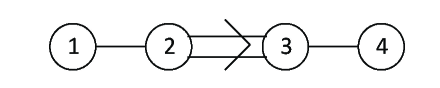
Figure 3: $F_{4}$ Dynkin diagram.

The following table lists the internal Chevalley modules that arise for maximal parabolic subgroups of $F_{4}$. We also indicate where the higher graded pieces arise earlier, except for those which are the standard actions of $SL(n)$. We write the 3rd fundamental representation of $Sp(6)$ as 14 (though caution the reader that the 2nd fundamental representation has the same dimension). The numbering and labeling conventions for the analogous charts for $D_{5}$, $E_{6}$, $E_{7}$, and $E_{8}$ remain in effect.

Node	Type of $[L,L]$	$i\,=\,1$	$i\,=\,2$	$i\,=\,3$	$i\,=\,4$
1	$Sp(6)$	14	Trivial
	$\dim\mathfrak{u}_{i}$	14	1
	action	$\varpi_{2}$
2	$SL(2)\times SL(3)$	Standard $\otimes$ Sym2	$C_{3}$ node 3
	$\dim\mathfrak{u}_{i}$	12	6	2
	action	$\varpi_{1}+2\varpi_{4}$	$2\varpi_{3}$	$\varpi$
3	$SL(3)\times SL(2)$	Tensor product	$B_{4}$ node 3
	$\dim\mathfrak{u}_{i}$	6	9	2	3
	action	$\varpi_{1}+\varpi_{4}$	$\varpi_{2}+2\varpi_{4}$	$\varpi_{4}$	$\varpi_{1}$
4	$SO(7)$	Spin	$B_{4}$ node 1
	$\dim\mathfrak{u}_{i}$	8	7
	action	$\varpi_{3}$	$\varpi_{1}$

5.10.1 $F_{4}$ Node 1

Here $P=LU$ where $U$ is a 15-dimensional Heisenberg group and $\mathfrak{u}=\mathfrak{u}_{1}\oplus\mathfrak{u}_{2}$, with $\dim\mathfrak{u}_{1}=14$ and $\dim\mathfrak{u}_{2}=1$. The semisimple part $[L,L]$ of $L$ is of type $Sp(6)$ and acts on $\mathfrak{u}_{1}$ as its 14-dimensional representation 3rd fundamental representation (corresponding to the long root). Its orbits are as follows.

Orbit Basepoint	Dimension	Coadjoint orbit intersected
1122+1220	14	2000
1222+1231	13	0100
1232	10	0001
1342	7	1000
0000	0	0000

The action on the one-dimensional piece $\mathfrak{u}_{2}$ has two orbits: zero and nonzero.

5.10.2 $F_{4}$ Node 2

Here $P=LU$ where $U$ is a 20-dimensional 3-step Heisenberg group and $\mathfrak{u}=\mathfrak{u}_{1}\oplus\mathfrak{u}_{2}\oplus\mathfrak{u}_{3}$, with $\dim\mathfrak{u}_{1}=12$, $\dim\mathfrak{u}_{2}=6$, and $\dim\mathfrak{u}_{3}=2$. The semisimple part $[L,L]$ of $L$ is of type $SL(2)\times SL(3)$ and acts on $\mathfrak{u}_{1}$ as the tensor product of the standard representation of the $SL(2)$ factor with the 6-dimensional symmetric square representation of the $SL(3)$ factor. It has the following orbits:

Orbit Basepoint	Dimension	Coadjoint orbit intersected
0100+0121+1111+1120	12	0200
0120+0122+1110	11	1010
0122+1110	10	2001
0121+1111+1120	10	0101
0122+1111+1120	9	0010
0121+1111	8	0002
0122+1120	8	2000
1111+1120	7	0100
0122+1121	7	0100
1121	6	0001
1122	4	1000
0000	0	0000

The symmetric square action of the $SL(3)$ factor on $\mathfrak{u}_{2}$ comes up earlier for $Sp(6)$, node 3, and has four orbits there of dimensions 6, 5, 3, and 0, with respective basepoints 021 + 111, 121, 221, and 000. The orbits here are the following:

Orbit Basepoint	Dimension	Coadjoint orbit intersected
1222+1231	6	0100
1232	5	0001
1242	3	1000
0000	0	0000

The action on $\mathfrak{u}_{3}$ is the standard action of $SL(2)$ has 2 orbits: zero and nonzero.

5.10.3 $F_{4}$ Node 3

Here $P=LU$ where $U$ is a 20-dimensional 4-step Heisenberg group and $\mathfrak{u}=\mathfrak{u}_{1}\oplus\mathfrak{u}_{2}\oplus\mathfrak{u}_{3}\oplus\mathfrak{u}_{4}$, with $\dim\mathfrak{u}_{1}=6$, $\dim\mathfrak{u}_{2}=9$, $\dim\mathfrak{u}_{3}=2$, and $\dim\mathfrak{u}_{4}=3$. The semisimple part $[L,L]$ of $L$ is of type $SL(3)\times SL(2)$ and acts on $\mathfrak{u}_{1}$ as the tensor product of the standard representations of the two factors. It has the following orbits:

Orbit Basepoint	Dimension	Coadjoint orbit intersected
0111+1110	6	0002
1111	4	0001
0000	0	0000

The action on $\mathfrak{u}_{2}$ is the tensor product of the standard representation of $SL(3)$ with the symmetric square representation of $SL(2)$, and came up earlier for $SO(5,4)$, node 3. It has orbits there of dimensions 9, 8, 7, 5, 4, and 0, with respective basepoints 0012 + 0111 + 1110, 0112 + 1110, 0112 + 1111, 1111, 1112, and 0000. It has the following orbits here:

Orbit Basepoint	Dimension	Coadjoint orbit intersected
0122+1121+1220	9	0010
1122+1220	8	2000
1122+1221	7	0100
1221	5	0001
1222	4	1000
0000	0	0000

The standard actions of $GL(2)$ and $GL(3)$, respectively, on $\mathfrak{u}_{3}$ and $\mathfrak{u}_{4}$ have two orbits each: zero and nonzero.

5.10.4 $F_{4}$ Node 4

Here $P=LU$ where $U$ is a 15-dimensional 2-step Heisenberg group and $\mathfrak{u}=\mathfrak{u}_{1}\oplus\mathfrak{u}_{2}$, with $\dim\mathfrak{u}_{1}=6$, $\dim\mathfrak{u}_{2}=8$ and $\dim\mathfrak{u}_{2}=7$. The semisimple part $[L,L]$ of $L$ is of type $SO(7)$ and acts on $\mathfrak{u}_{1}$ as its spin representation, with the following orbits:

Orbit Basepoint	Dimension	Coadjoint orbit intersected
0121+1111	8	0002
1231	7	0001
0000	0	0000

The action on $\mathfrak{u}_{2}$ is the 7-dimensional vector action, which came up previously for $SO(5,4)$, node 1. It has orbits there of dimensions 7, 6, and 0, with respective basepoints 1111, 1222, and 0000. Its orbits here are:

Orbit Basepoint	Dimension	Coadjoint orbit intersected
1232	7	0001
2342	6	1000
0000	0	0000

5.11 Type $G_{2}$

$G_{2}$ Dynkin diagram.

The following table lists the internal Chevalley modules for the two conjugacy classes of maximal parabolic subgroups of $G_{2}$. The actions on $\mathfrak{u}_{2}$ are trivial, while the action for node 1 on $\mathfrak{u}_{3}$ is the 2-dimensional standard representation of $SL(2)$ (it has two orbits: zero and nonzero). We list the actions below and the orbits on $\mathfrak{u}_{1}$, which are most interesting in the case of the symmetric cube action for node 2.

Node	Type of $[L,L]$	$i\,=\,1$	$i\,=\,2$	$i\,=\,3$
1	$SL(2)$	Standard	Trivial	Standard
	$\dim\mathfrak{u}_{i}$	2	1	2
	action	$\varpi$		($SL(3)$ node 1)
2	$SL(2)$	Symmetric cube	Trivial
	$\dim\mathfrak{u}_{i}$	4	1
	action	$3\varpi$

Orbit Basepoint	Dimension	Coadjoint orbit intersected
Node 1
11	2	10
00	0	00
Node 2
01+31	4	02
21	3	10
31	2	01
00	0	00

ArtinE.Geometric algebraInterscience Publishers, Inc.New York-London1957@book{artin, author = {Artin, E.}, title = {Geometric Algebra}, publisher = {Interscience Publishers, Inc.}, place = {New York-London}, date = {1957}} AtkinA. O. L.LehnerJ.Hecke operators on $\Gamma_{0}(m)$Math. Ann.1851970134–160ISSN 0025-5831Review MathReviews@article{atkinlehner, author = {Atkin, A. O. L.}, author = {Lehner, J.}, title = {Hecke operators on $\Gamma\sb{0}(m)$}, journal = {Math. Ann.}, volume = {185}, date = {1970}, pages = {134–160}, issn = {0025-5831}, review = {\MR{0268123 (42 \#3022)}}} BateBrandonRutgers University Ph.D. thesis, in preparation@thesis{bate, author = {Bate, Brandon}, note = {Rutgers University Ph.D. thesis, in preparation}} BhargavaA.Higher composition laws i: a new view on gauss composition, and quadratic generalizationsAnnals of Mathematics1592004217–250@article{bhargava, author = {Bhargava, A.}, title = {Higher composition laws I: A new view on Gauss composition, and quadratic generalizations}, journal = {Annals of Mathematics}, volume = {159}, date = {2004}, pages = {217-250}} BorhoW.BrylinskiJ.L.Differential operators on homogeneous spaces, i Invent. Math.691982437–476@article{borho, author = {Borho, W.}, author = {Brylinski, J.L.}, title = {Differential operators on homogeneous spaces, I}, journal = { Invent. Math.}, volume = {69}, date = {1982}, pages = {437-476}} BumpDanielAutomorphic forms on ${\rm GL}(3,{\bf R})$Lecture Notes in Mathematics1083Springer-VerlagBerlin1984xi+184ISBN 3-540-13864-1Review MathReviews@book{bumpgl3, author = {Bump, Daniel}, title = {Automorphic forms on ${\rm GL}(3,{\bf R})$}, series = {Lecture Notes in Mathematics}, volume = {1083}, publisher = {Springer-Verlag}, place = {Berlin}, date = {1984}, pages = {xi+184}, isbn = {3-540-13864-1}, review = {\MR{765698 (86g:11028)}}} DjokovicD. Z.Classification of trivectors of an eight-dimensional real vector spaceLinear Multilinear Algebra133–391983@article{djokovic, author = {Djokovic, D. Z.}, title = {Classification of trivectors of an eight-dimensional real vector space}, journal = {Linear Multilinear Algebra}, volume = {13}, pages = {3–39}, date = {1983}} GinzburgDavidHundleyJosephConstructions of global integrals in the exceptional groupshttp://arxiv.org/abs/1108.1401@article{ginzhund, author = {Ginzburg, David}, author = {Hundley, Joseph}, title = {Constructions of global integrals in the exceptional groups}, note = {\url{http://arxiv.org/abs/1108.1401}}} de GraafWillem A.Computing representatives of nilpotent orbits of $\theta$-groupshttp://arxiv.org/abs/0905.3149@article{deG, author = {de Graaf, Willem A.}, title = {Computing representatives of nilpotent orbits of $\theta$-groups}, note = {\url{http://arxiv.org/abs/0905.3149}}} GanWee TeckGrossBenedictSavinGordanFourier coefficients of modular forms on $G_{2}$Duke Math. J.11520021105–169ISSN 0012-7094Review MathReviewsDocument@article{ggs, author = {Gan, Wee Teck}, author = {Gross, Benedict}, author = {Savin, Gordan}, title = {Fourier coefficients of modular forms on $G_2$}, journal = {Duke Math. J.}, volume = {115}, date = {2002}, number = {1}, pages = {105–169}, issn = {0012-7094}, review = {\MR{1932327 (2004a:11036)}}, doi = {10.1215/S0012-7094-02-11514-2}} GourevitchDmitrySahiSiddharthaAnnihilator varieties, highest derivatives, whittaker functionals, and rank for unitary representations of $GL(n,{\mathbb{R}})$http://arxiv.org/abs/1106.0454@article{Gurevich-Sahi, author = {Gourevitch, Dmitry}, author = {Sahi, Siddhartha}, title = {Annihilator varieties, highest derivatives, Whittaker functionals, and rank for unitary representations of $GL(n,\R)$}, note = {\url{http://arxiv.org/abs/1106.0454}}} GreenMichael B.MillerStephen D.VanhovePierreSmall representations, string instantons, and fourier modes of eisenstein series (with an appendix by d. ciubotaru and p. trapa)http://arxiv.org/abs/1111.2983@article{GMV, author = {Green, Michael B.}, author = {Miller, Stephen D.}, author = {Vanhove, Pierre}, title = {Small representations, string instantons, and Fourier modes of Eisenstein series (with an appendix by D. Ciubotaru and P. Trapa)}, note = {\url{http://arxiv.org/abs/1111.2983}}} HarisStephen J.Some irreducible representations of exceptional algebraic groupsAmerican Journal of Mathematics931197175–106@article{haris, author = {Haris, Stephen J.}, title = {Some Irreducible Representations of Exceptional Algebraic Groups}, journal = {American Journal of Mathematics}, volume = {93}, number = {1}, date = {1971}, pages = {75-106}} HeckeErichLectures on dirichlet series, modular functions and quadratic formsEdited by Bruno Schoeneberg; With the collaboration of Wilhelm MaakVandenhoeck & RuprechtG\"ottingen198398ISBN 3-525-40727-0Review MR 85c:11042@book{Hecke, author = {Hecke, Erich}, title = {Lectures on Dirichlet series, modular functions and quadratic forms}, note = {Edited by Bruno Schoeneberg; With the collaboration of Wilhelm Maak}, publisher = {Vandenhoeck \& Ruprecht}, place = {G\"ottingen}, date = {1983}, pages = {98}, isbn = {3-525-40727-0}, review = {MR 85c:11042}} @article{igusa}

author=Igusa, J., title=A classification of spinors up to dimension twelve, journal=American Journal of Mathematics, volume=92,year=1970, pages=997-1028,

JacquetH.LanglandsR. P.Automorphic forms on ${\rm GL}(2)$Lecture Notes in Mathematics, Vol. 114Springer-VerlagBerlin1970vii+548Review MathReviews@book{jacquetlanglands, author = {Jacquet, H.}, author = {Langlands, R. P.}, title = {Automorphic forms on ${\rm GL}(2)$}, series = {Lecture Notes in Mathematics, Vol. 114}, publisher = {Springer-Verlag}, place = {Berlin}, date = {1970}, pages = {vii+548}, review = {\MR{0401654 (53 \#5481)}}} JiangDihuaDegree $16$ standard $L$-function of ${\rm GSp}(2)\times{\rm GSp}(2)$Mem. Amer. Math. Soc.1231996588viii+196ISSN 0065-9266Review MathReviews@article{jiang, author = {Jiang, Dihua}, title = {Degree $16$ standard $L$-function of ${\rm GSp}(2)\times{\rm GSp}(2)$}, journal = {Mem. Amer. Math. Soc.}, volume = {123}, date = {1996}, number = {588}, pages = {viii+196}, issn = {0065-9266}, review = {\MR{1342020 (97d:11081)}}} JiangDihuaRallisStephenFourier coefficients of eisenstein series of the exceptional group of type $G_{2}$Pacific J. Math.18119972281–314ISSN 0030-8730Review MathReviews@article{jiang-rallis, author = {Jiang, Dihua}, author = {Rallis, Stephen}, title = {Fourier coefficients of Eisenstein series of the exceptional group of type $G_2$}, journal = {Pacific J. Math.}, volume = {181}, date = {1997}, number = {2}, pages = {281–314}, issn = {0030-8730}, review = {\MR{1486533 (99d:11054)}}} JosephA.On the associated variety of a primitive idealJour. of Algebra931985509–523@article{joseph, author = {Joseph, A.}, title = {On the associated variety of a primitive ideal}, journal = {Jour. of Algebra}, volume = {93}, date = {1985}, pages = {509-523}} KazhdanD.PolishchukA.Minimal representations: spherical vectors and automorphic functionalstitle={Algebraic groups and arithmetic}, publisher={Tata Inst. Fund. Res.}, place={Mumbai}, 2004127–198Review MathReviews@article{kazhpoli, author = {Kazhdan, D.}, author = {Polishchuk, A.}, title = {Minimal representations: spherical vectors and automorphic functionals}, conference = {title={Algebraic groups and arithmetic}, }, book = {publisher={Tata Inst. Fund. Res.}, place={Mumbai}, }, date = {2004}, pages = {127–198}, review = {\MR{2094111 (2005i:22018)}}} KrutelevichS.Jordan algebras, exceptional groups, and bhargava compositionJ. Algebra3142007924–977arXiv:math/0411104@article{krutelevich, author = {Krutelevich, S.}, title = {Jordan algebras, exceptional groups, and Bhargava composition}, journal = {J. Algebra}, volume = {314}, date = {2007}, pages = {924-977}, note = {arXiv:math/0411104}} LiJian-ShuNonexistence of singular cusp formsCompositio Math.831992143–51ISSN 0010-437XReview MathReviews@article{jsli, author = {Li, Jian-Shu}, title = {Nonexistence of singular cusp forms}, journal = {Compositio Math.}, volume = {83}, date = {1992}, number = {1}, pages = {43–51}, issn = {0010-437X}, review = {\MR{1168122 (93f:11040)}}} LittelmannP.An effective method to classify nilpotent orbitstitle={Algorithms in algebraic geometry and applications (Santander, 1994)}, series={Progr. Math.}, volume={143}, publisher={Birkh\"auser}, place={Basel}, 1996255–269Review MathReviews@article{littelmann, author = {Littelmann, P.}, title = {An effective method to classify nilpotent orbits}, conference = {title={Algorithms in algebraic geometry and applications (Santander, 1994)}, }, book = {series={Progr. Math.}, volume={143}, publisher={Birkh\"auser}, place={Basel}, }, date = {1996}, pages = {255–269}, review = {\MR{1414453 (98a:20041)}}} MaassHansÜber eine neue art von nichtanalytischen automorphen funktionen und die bestimmung dirichletscher reihen durch funktionalgleichungenGermanMath. Ann.1211949141–183Review MR 11,163c@article{Maass, author = {Maass, Hans}, title = {\"Uber eine neue Art von nichtanalytischen automorphen Funktionen und die Bestimmung Dirichletscher Reihen durch Funktionalgleichungen}, language = {German}, journal = {Math. Ann.}, volume = {121}, date = {1949}, pages = {141\ndash 183}, review = {MR 11,163c}} MatumotoHisayosiWhittaker vectors and associated varietiesInvent. Math.8919871219–224ISSN 0020-9910Review MathReviewsDocument@article{matumoto, author = {Matumoto, Hisayosi}, title = {Whittaker vectors and associated varieties}, journal = {Invent. Math.}, volume = {89}, date = {1987}, number = {1}, pages = {219–224}, issn = {0020-9910}, review = {\MR{892192 (88k:17022)}}, doi = {10.1007/BF01404678}} MillerStephen D.SchmidWilfriedAutomorphic distributions, $L$-functions, and voronoi summation for ${\rm GL}(3)$Ann. of Math. (2)16420062423–488ISSN 0003-486XReview MathReviews@article{voronoi, author = {Miller, Stephen D.}, author = {Schmid, Wilfried}, title = {Automorphic distributions, $L$-functions, and Voronoi summation for ${\rm GL}(3)$}, journal = {Ann. of Math. (2)}, volume = {164}, date = {2006}, number = {2}, pages = {423–488}, issn = {0003-486X}, review = {\MR{2247965}}} MœglinC.WaldspurgerJ.-L.Modèles de whittaker dégénérés pour des groupes $p$-adiquesFrenchMath. Z.19619873427–452ISSN 0025-5874Review MathReviewsDocument@article{Mowa, author = {M{\oe}glin, C.}, author = {Waldspurger, J.-L.}, title = {Mod\`eles de Whittaker d\'eg\'en\'er\'es pour des groupes $p$-adiques}, language = {French}, journal = {Math. Z.}, volume = {196}, date = {1987}, number = {3}, pages = {427–452}, issn = {0025-5874}, review = {\MR{913667 (89f:22024)}}, doi = {10.1007/BF01200363}} Piatetski-ShapiroI. I.Multiplicity one theoremstitle={Automorphic forms, representations and $L$-functions (Proc. Sympos. Pure Math., Oregon State Univ., Corvallis, Ore., 1977), Part 1}, series={Proc. Sympos. Pure Math., XXXIII}, publisher={Amer. Math. Soc.}, place={Providence, R.I.}, 1979209–212Review MathReviews@article{psmult, author = {Piatetski-Shapiro, I. I.}, title = {Multiplicity one theorems}, conference = {title={Automorphic forms, representations and $L$-functions (Proc. Sympos. Pure Math., Oregon State Univ., Corvallis, Ore., 1977), Part 1}, }, book = {series={Proc. Sympos. Pure Math., XXXIII}, publisher={Amer. Math. Soc.}, place={Providence, R.I.}, }, date = {1979}, pages = {209–212}, review = {\MR{546599 (81m:22027)}}} L.Popov,V.Classification of the spinors of dimension fourteenUspekhi Mat. Nauk3219771(193) 199 –200@article{popov, author = {Popov,V. L.}, title = {Classification of the spinors of dimension fourteen}, journal = {Uspekhi Mat. Nauk}, volume = {32}, date = {1977}, number = {1(193) }, pages = {199 -200}} RichardsonRogerRöhrleGerhardSteinbergRobertParabolic subgroups with abelian unipotent radicalInvent. Math.11019923649–671ISSN 0020-9910Review MathReviewsDocument@article{rrs, author = {Richardson, Roger}, author = {R{\"o}hrle, Gerhard}, author = {Steinberg, Robert}, title = {Parabolic subgroups with abelian unipotent radical}, journal = {Invent. Math.}, volume = {110}, date = {1992}, number = {3}, pages = {649–671}, issn = {0020-9910}, review = {\MR{1189494 (93j:20092)}}, doi = {10.1007/BF01231348}} RöhrleGerhardOrbits in internal chevalley modulestitle={Groups, combinatorics \& geometry}, address={Durham}, date={1990}, series={London Math. Soc. Lecture Note Ser.}, volume={165}, publisher={Cambridge Univ. Press}, place={Cambridge}, 1992311–315Review MathReviews@article{rohrleinternal, author = {R{\"o}hrle, Gerhard}, title = {Orbits in internal Chevalley modules}, conference = {title={Groups, combinatorics \& geometry}, address={Durham}, date={1990}, }, book = {series={London Math. Soc. Lecture Note Ser.}, volume={165}, publisher={Cambridge Univ. Press}, place={Cambridge}, }, date = {1992}, pages = {311–315}, review = {\MR{1200268}}} RöhrleGerhard E.On extraspecial parabolic subgroupstitle={Linear algebraic groups and their representations (Los Angeles, CA, 1992)}, series={Contemp. Math.}, volume={153}, publisher={Amer. Math. Soc.}, place={Providence, RI}, 1993143–155Review MathReviews@article{rohrle, author = {R{\"o}hrle, Gerhard E.}, title = {On extraspecial parabolic subgroups}, conference = {title={Linear algebraic groups and their representations (Los Angeles, CA, 1992)}, }, book = {series={Contemp. Math.}, volume={153}, publisher={Amer. Math. Soc.}, place={Providence, RI}, }, date = {1993}, pages = {143–155}, review = {\MR{1247502 (94k:20082)}}} RöhrleGerhard E.On the structure of parabolic subgroups in algebraic groupsJ. Algebra1571993180–115ISSN 0021-8693Review MathReviewsDocument@article{MR1219660, author = {R{\"o}hrle, Gerhard E.}, title = {On the structure of parabolic subgroups in algebraic groups}, journal = {J. Algebra}, volume = {157}, date = {1993}, number = {1}, pages = {80–115}, issn = {0021-8693}, review = {\MR{1219660 (94d:20053)}}, doi = {10.1006/jabr.1993.1092}} SavinGordanDual pair $G_{J}\times PGL_{2}$; $G_{J}$ is the automorphism group of a jordan algebra $J$.Invent. Math.1181994141–160@article{savin, author = {Savin, Gordan}, title = {Dual pair $G_J \times PGL_2$; $G_J$ is the automorphism group of a Jordan algebra $J$.}, journal = {Invent. Math.}, volume = {118}, date = {1994}, pages = {141–160}} SavinGordanWoodburyMichaelStructure of internal modules and a formula for the spherical vector of minimal representationsJ. Algebra31220072755–772ISSN 0021-8693Review MathReviewsDocument@article{savinwoodbury, author = {Savin, Gordan}, author = {Woodbury, Michael}, title = {Structure of internal modules and a formula for the spherical vector of minimal representations}, journal = {J. Algebra}, volume = {312}, date = {2007}, number = {2}, pages = {755–772}, issn = {0021-8693}, review = {\MR{2333183 (2008g:20102)}}, doi = {10.1016/j.jalgebra.2007.01.014}} ShahidiFreydoonA proof of langlands’ conjecture on plancherel measures; complementary series for $p$-adic groupsAnn. of Math. (2)13219902273–330ISSN 0003-486XReview MathReviewsDocument@article{shahidi, author = {Shahidi, Freydoon}, title = {A proof of Langlands' conjecture on Plancherel measures; complementary series for $p$-adic groups}, journal = {Ann. of Math. (2)}, volume = {132}, date = {1990}, number = {2}, pages = {273–330}, issn = {0003-486X}, review = {\MR{1070599 (91m:11095)}}, doi = {10.2307/1971524}} ShalikaJ. A.The multiplicity one theorem for ${\rm GL}_{n}$Ann. of Math. (2)1001974171–193ISSN 0003-486XReview MathReviews@article{shalika, author = {Shalika, J. A.}, title = {The multiplicity one theorem for ${\rm GL}\sb{n}$}, journal = {Ann. of Math. (2)}, volume = {100}, date = {1974}, pages = {171–193}, issn = {0003-486X}, review = {\MR{0348047 (50 \#545)}}}