Finite wave vector pairing in doped two-leg ladders

Abstract

We consider the effects of Umklapp processes in doped two-leg fermionic ladders. These may emerge either at special band fillings or as a result of the presence of external periodic potentials. We show that such Umklapp processes can lead to profound changes of physical properties and in particular stabilize pair-density wave phases.

I Introduction

As is well illustrated by the example of the one-dimensional Hubbard model book , Umklapp processes in strongly correlated systems may lead to a profound restructuring of the ground state. Indeed, at half filling when the Fermi wave vector is such that $4k_{F}=2\pi$, Umklapp scattering processes connect opposite Fermi points and open a spectral gap for single-particle excitations. In a similar way Umklapp processes in undoped two-leg fermionic ladders are known to generate a variety of insulating states balents ; O(8) ; tsuchiizu ; fradkin . In both cases these Umklapp processes become relevant at the particular density of one electron per site, independently of the details of the interactions. In multi-band systems such as the 2-leg ladder there are other kinds of Umklapp processes that can connect Fermi points at certain other band fillings, which generally depend on the microscopic details of both the band structure and the interactions.

One example where such processes may play a crucial role is the “telephone number compound” ${\rm Sr_{14-x}Ca_{x}Cu_{24}O_{41}}$ SrCaCuO1 ; SrCaCuO2 . X-ray scattering techniques have established the presence of a standing wave in the hole density without a significant lattice distortion in this material SrCaCuO1 . The simplest explanation for these findings is a crystalline state of pairs of holes PDW ; Poilblanc . The physical origin of the hole crystal is likely to be the long-ranged Coulomb interaction between ladders. Treating this interladder Coulomb interaction in a mean-field approximation leads to a model of decoupled ladders subject to a (self-consistent) periodic potential Poilblanc . The latter introduces Umklapp processes and an important question of current interest is what effects these have both on the ground state and excitations of the ladders.

A second example in which Umklapp processes may be important is $x=1/8$ doped La_2-xSr_xCuO₄berg_et_al_2007 . In this material regular ”stripe” order is formed below a critical temperature  Stripes . Stripes in neighboring planes are perpendicular to each other and are shifted by one lattice spacing Tranquada1 . The unit cell in the CuO planes contains four sites, which can be thought of as forming two undoped and two doped chains of atoms. Hence the period in the direction perpendicular to the CuO planes is four. On the other hand, the doped chains are 3/4 filled. As a result the period of the potential induced by the neighboring planes is also four, which coincides with the average distance between holes in the doped chains. A simple model describing this situation is given by doped 2-leg ladders in presence of a periodic potential. It is well established that La_1.875Sr_0.125CuO₄ exhibits rather exotic 2D superconducting behavior as a result of the CuO planes being effectively decoupled from one another Tranquada2 ; Basov . Similar dynamical layer decoupling has recently been observed in heavy fermion superconductor CeRhIn₅ CeRhIn .

Umklapp processes can in principle also be induced by imposing external periodic potentials. This has recently been demonstrated by adsorbing noble gas monolayers on the surface on carbon nanotubes cobden .

From a theoretical point of view, there is one particular case, in which it is known that Umklapp processes have very interesting physical consequences. This occurs in the so-called Kondo-Heisenberg model zachar ; berg . The latter describes a situation where the two legs of the ladder are inequivalent. Leg 1 is half-filled and as a consequence of Umklapp interactions has a large Mott gap, while leg 2 has a density of less than one electron per site. At low energies tunneling between the legs is not allowed due to the presence of a large Mott gap in leg 1, but virtual processes lead to a Heisenberg exchange interaction between electron spins on the two legs. The resulting model describing the low-energy physics of such a 2-leg ladder consists of a spin S=1/2 Heisenberg chain (leg 1) interacting via exchange interactions with a one-dimensional electron gas (1DEG, leg 2). Generically the Fermi momentum of the 1DEG will be incommensurate with the lattice. It was demonstrated in zachar that this Kondo-Heisenberg model exhibits quasi-long-range order of particular composite order parameter at a finite wave vector. More recently it was shown berg that there also is quasi-long-range superconducting order with wave number $\pi$, consituting an example of a 1D Fulde-Ferrell-Larkin-Ovchinnikov state FFLO in the absence of a magnetic field. In very recent work FradkinArx it was demonstrated that the PDW state is in fact much more general and in particular does not require the legs to be inequivalent.

In the following we consider spin-1/2 fermions on a two-leg ladder with Hubbard and nearest-neighbor density-density interactions. In addition we allow an external periodic potential to be present. The Hamiltonian is given by

$$H_{\rm ladd}(K) = -t\sum_{n,\alpha}\sum_{j=1}^{2}a^{\dagger}_{j,n+1,\alpha}a_{j,n,\alpha}+a^{\dagger}_{j,n,\alpha}a_{j,n+1,\alpha}-t_{\perp}\sum_{n,\alpha}a^{\dagger}_{1,n,\alpha}a_{2,n,\alpha}+a^{\dagger}_{2,n,\alpha}a_{1,n,\alpha}+U\sum_{j,l}n_{j,l,\uparrow}n_{j,l,\downarrow}$$ (1)

$$+ V_{\perp}\sum_{l}n_{1,l}n_{2,l}+V_{\parallel}\sum_{j,l}n_{j,l}n_{j,l+1}+\sum_{j,l}W_{j}\cos(Kl)\ n_{j,l},$$

where $a_{j,n,\alpha}$ are annihilation operators for spin-$\alpha$ electrons on site $n$ of leg $j$ of the ladder and $n_{j,l,\alpha}=a^{\dagger}_{j,l,\alpha}a_{j,l,\alpha}$. $U$ is the Hubbard interaction strength, $V_{\perp}$ and $V_{\parallel}$ are the density-density interaction strengths along the rung and leg directions respectively and the periodic potential is characterized by its strength on each leg $W_{1,2}$ and the wavenumber of its modulation, $K$. The lattice model (1) has U(1)$\times$SU(2) symmetry, with an additional $\mathbb{Z}_{2}$ symmetry if $W_{1}=W_{2}$. It is useful to rewrite the periodic potential term as

$$\sum_{l}\cos(Kl)\Big{[}W_{+}(n_{1,l}+n_{2,l})+W_{-}(n_{1,l}-n_{2,l})\Big{]},$$ (2)

where $W_{\pm}=(W_{1}\pm W_{2})/2$. A nonzero $W_{-}$ breaks the symmetry between the two legs of the ladder. In the following we consider a case where $W_{-}=0$ (“$4k_{b}$ Umklapp”) and one where $W_{+}=0$ (“$3k_{b}+k_{ab}$ Umklapp”). A schematic diagram of the ladder geometry can be seen in Fig. 1. In order see which wave numbers $K$ will lead to the most pronounced effects for weak interactions and small $W_{1,2}$ it is useful to consider the band structure of $H_{\rm ladd}$ in the absence of interactions. It is useful to introduce the bonding ($b$) and antibonding ($ab$) variables by

$$c_{j,n,\alpha}=\frac{1}{\sqrt{2}}\left(a_{1,n,\alpha}-(-1)^{j}a_{2,n,\alpha}\right)\ ,$$ (3)

where $j=1,2=b,ab$. In terms of these operators the non-interacting tight-binding Hamiltonian $H_{\rm ladd,0}$ is diagonal in momentum space

$$H_{\rm ladd,0}=\sum_{j=1}^{2}\sum_{k}\epsilon_{j}(k)c^{\dagger}_{j,\alpha}(k)c_{j,\alpha}(k)\ ,$$ (4)

where $c_{j,\alpha}(k)=L^{-1/2}\sum_{n}e^{ikn}c_{j,n,\alpha}$ and

$$\epsilon_{1}(k)=-2t\cos(k)-t_{\perp}\ ,\quad\epsilon_{2}(k)=-2t\cos(k)+t_{\perp}\ .$$ (5)

The corresponding band structure is shown in Fig. 1(b). For weak interactions the low energy degrees of freedom occur in the vicinities of $nk_{b}$ and $nk_{ab}$ where $n$ in an integer and $k_{b}$, $k_{ab}$ are the Fermi momenta of the bonding and antibonding bands respectively. It is then clear that external potentials with wave numbers $K=n_{1}k_{b}+n_{2}k_{ab}$ will affect the low-energy degrees of freedom most strongly. In the following we concentrate on the cases $K=3k_{b}+k_{ab}$ and $K=4k_{b}$. As we will see, in the case of strong interactions but small $t_{\perp}$ an analogous picture applies.

(a)

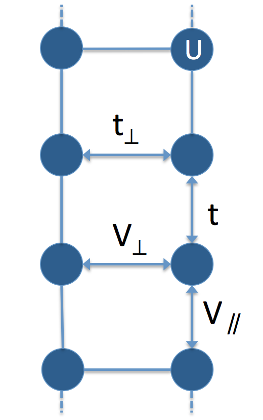
(b)

Figure 1: (a): Extended Hubbard Ladder with different leg and rung hopping amplitudes and density-density interactions. (b): The non-interacting band structure for the tight-binding model on the ladder, with the Fermi wavevectors labelled.

This paper is organized as follows. In Section II we derive the low-energy effective field theories in the “band” and “chain” limits of the Hamiltonian (1) and discuss how we account for the external periodic potential. In Section III we consider the $4k_{b}$ Umklapp process in both band and chain representations of the model. By means of renormalization group methods we derive the effective low energy theories describing the strong coupling fixed points. In Section IV we analyze the effects of the $3k_{b}+k_{ab}$ Umklapp process at low energies in both band and chain representations of the model. Section V presents density matrix renormalization group (DMRG) calculations in intermediate parameter regimes. Section VI contains the conclusions. A number of technical points are discussed in several appendices.

II Low-Energy Description

There are two complementary ways of deriving a field theory description of the lattice Hamiltonian (1), each of which applies to a particular limit of the model. One may start by considering the non-interacting Hamiltonian, diagonalizing the tight-binding model by transforming to bonding and antibonding variables and subsequently treating the interaction using perturbative renormalization group methods Fabr93 ; balents ; schulz96 ; lin . Hereinafter this approach will be called the “band representation”. Alternatively, one may start by considering two strongly interacting uncoupled chains and treat the across rung hopping $t_{\perp}$ and density-density interaction $V_{\perp}$ as perturbations dima ; amt . This approach will be referred to as the “chain representation”. In the following subsections we summarize both approaches in turn.

II.1 The Band Representation $U,V_{j}\ll t,t_{\perp}$

Here the starting point is the tight-binding model obtained by dropping all interaction terms in the Hamiltonian (1). The resulting model is diagonalized in terms of the bonding and antibonding ($b/ab$) variables (3), resulting in split bonding and antibonding bands (4) as depicted in Fig. 1(b). As we are interested in the low-energy behaviour of the system, we linearize the spectrum around the Fermi points. The low-energy projections of the lattice fermion operators are then

$$c_{j,n,\alpha}\sim\sqrt{a_{0}}\left[R_{j,\alpha}(x)e^{ik_{j}x}+L_{j,\alpha}(x)e^{-ik_{j}x}\right],$$ (6)

where $L(x)$ and $R(x)$ are left and right moving fermion fields close to the Fermi points, $k_{b}$ ($k_{ab}$) is the Fermi wavevector in the bonding (antibonding) band and $a_{0}$ is the lattice spacing, which serves as the short-distance cut-off of the theory. The interactions are conveniently expressed in terms of currents balents , which following Ref. CCL we define as

$$I_{ij}^{R} = \frac{1}{2}R_{i,\alpha}\ \epsilon_{\alpha\beta}\ R_{j,\beta}\ ,\qquad I^{aR}_{ij}=\frac{1}{2}R_{i,\alpha}(\epsilon\sigma^{a})_{\alpha\beta}R_{j,\beta}\ ,$$ (7)

$$J_{ij}^{R} = \frac{1}{2}R^{\dagger}_{i,\alpha}\ R_{j,\alpha}\ ,\qquad~{}~{}\quad J^{aR}_{ij}=\frac{1}{2}R^{\dagger}_{i,\alpha}\sigma^{a}_{\alpha\beta}R_{j,\beta},$$ (8)

and similarly for left-moving fermion fields with $R\leftrightarrow L$. The low-energy Hamiltonian then takes the form $H=\int dx\ \left[{\cal H}_{0}+{\cal H}_{U}+{\cal H}_{W}\right]$, where

$${\cal H}_{0} = \sum_{j=1}^{2}v_{j}\Big{(}-iR^{\dagger}_{j,\alpha}\partial_{x}R_{j,\alpha}+iL^{\dagger}_{j,\alpha}\partial_{x}L_{j,\alpha}\Big{)}\ ,$$

$${\cal H}_{U} = \sum_{i,j}\tilde{c}^{\rho}_{ij}J_{ij}^{R}J_{ij}^{L}-\tilde{c}^{\sigma}_{ij}J^{aR}_{ij}J^{aL}_{ij}+\sum_{i\neq j}\tilde{f}^{\rho}_{ij}J_{ii}^{R}J_{jj}^{L}-\tilde{f}^{\sigma}_{ij}J^{aR}_{ii}J^{aL}_{jj}\ ,$$

$${\cal H}_{W} = \sum_{P\in S}\sum_{\sigma=\pm}W_{\sigma,P}\ \delta_{K,P}\left[\rho^{(\sigma)}_{P}(x)+{\rm h.c.}\right].$$ (9)

Here $\rho^{(\sigma)}_{P}(x)$ are the Fourier components of the low-energy projections of $n_{1,l}\pm n_{2,l}$, c.f. Eq. (2), with momenta close to $P$; these components are discussed in some detail in Appendix A. In the following we consider “$4k_{F}$” components with wave numbers around $S=\{4k_{b},~{}4k_{ab},~{}3k_{b}+k_{ab},~{}3k_{ab}+k_{b}\}$. The “$2k_{F}$”-response is generally blocked by the presence of a spin gap in doped Hubbard ladders, see e.g. Appendix A.1, and we shall not consider them here. The $4k_{F}$ components of the density are obtained by integrating out the high-energy degrees of freedom perturbatively in $U$, see Appendix B, and are given in terms of the currents as

$$\rho^{(+)}_{4k_{b}}(x)+{\rm h.c.} = \big{(}I_{11}^{L}\big{)}^{\dagger}I_{11}^{R}+\big{(}I_{11}^{R}\big{)}^{\dagger}I_{11}^{L}\ ,$$

$$\rho^{(+)}_{4k_{ab}}(x)+{\rm h.c.} = \big{(}I_{22}^{L}\big{)}^{\dagger}I_{22}^{R}+\big{(}I_{22}^{R}\big{)}^{\dagger}I_{22}^{L}\ ,$$

$$\rho^{(+)}_{2k_{b}+2k_{ab}}(x)+{\rm h.c.} = 8\left\{\big{(}I_{12}^{L}\big{)}^{\dagger}I_{21}^{R}+\big{(}I_{21}^{R}\big{)}^{\dagger}I_{12}^{L}\right\},$$

$$\rho^{(-)}_{k_{b}+3k_{ab}}(x)+{\rm h.c.} = 2\left\{\big{(}I_{22}^{L}\big{)}^{\dagger}I^{R}_{21}+\big{(}I_{21}^{L}\big{)}^{\dagger}I^{R}_{22}+\big{(}I_{22}^{R}\big{)}^{\dagger}I^{L}_{21}+\big{(}I_{21}^{R}\big{)}^{\dagger}I^{L}_{22}\right\}\ ,$$

$$\rho^{(-)}_{3k_{b}+k_{ab}}(x)+{\rm h.c.} = 2\left\{\big{(}I_{11}^{L}\big{)}^{\dagger}I^{R}_{12}+\big{(}I_{12}^{L}\big{)}^{\dagger}I^{R}_{11}+\big{(}I_{11}^{R}\big{)}^{\dagger}I^{L}_{12}+\big{(}I_{12}^{R}\big{)}^{\dagger}I^{L}_{11}\right\}.$$ (10)

The initial conditions for the coupling constants defined in (9) for the extended Hubbard model are

$$\tilde{c}_{ii}^{\rho} = U+V_{\perp}+4V_{\parallel}\left[1-\frac{1}{2}\cos(2k_{i}a_{0})\right],$$

$$\tilde{c}_{ij}^{\rho} = U-V_{\perp}+4V_{\parallel}\left[\cos((k_{b}-k_{ab})a_{0})-\frac{1}{2}\cos((k_{b}+k_{ab})a_{0})\right],$$

$$\tilde{f}_{ij}^{\rho} = U+3V_{\perp}+4V_{\parallel}\left[1-\frac{1}{2}\cos((k_{b}+k_{ab})a_{0})\right],$$

$$\tilde{c}_{ii}^{\sigma} = U+V_{\perp}+2V_{\parallel}\cos(2k_{i}a_{0}),$$

$$\tilde{f}_{ij}^{\sigma} = \tilde{c}_{ij}^{\sigma}=U-V_{\perp}+2V_{\parallel}\cos((k_{b}+k_{ab})a_{0}).$$

The analysis which we carry out in the band representation requires the bosonized Hamiltonian. Following Ref. GNT , we bosonize the Hamiltonian according to

$$R_{d,\sigma}\sim\frac{\kappa_{d,\sigma}}{\sqrt{2\pi}}e^{i\sqrt{4\pi}\varphi_{d,\sigma}}\ ,\qquad L_{d,\sigma}\sim\frac{\kappa_{d,\sigma}}{\sqrt{2\pi}}e^{-i\sqrt{4\pi}\bar{\varphi}_{d,\sigma}},\qquad d=1,2=b,ab,$$ (11)

where $\varphi_{d,\sigma}$ ($\bar{\varphi}_{d,\sigma}$) is the right (left) chiral component of a canonical boson field and $\{\kappa_{d,\sigma},\kappa_{d^{\prime},\sigma^{\prime}}\}=2\delta_{d,d^{\prime}}\delta_{\sigma,\sigma^{\prime}}$ are Klein factors to ensure the anti-commutation of different species of fermions. The boson fields have commutation relations

$$[\varphi_{d,\sigma}(x),\varphi_{d^{\prime},\sigma^{\prime}}(x^{\prime})]=-[\bar{\varphi}_{d,\sigma}(x),\bar{\varphi}_{d^{\prime},\sigma^{\prime}}(x^{\prime})]=\frac{i}{4}{\rm sgn}(x-x^{\prime})\delta_{d,d^{\prime}}\delta_{\sigma,\sigma^{\prime}},\quad[\varphi_{d,\sigma}(x),\bar{\varphi}_{d^{\prime},\sigma^{\prime}}(x^{\prime})]=\frac{i}{4}\delta_{d,d^{\prime}}\delta_{\sigma,\sigma^{\prime}},$$ (12)

which enforce anti-commutation relations for fermions of the same species. Then, we change to spin and charge bosons according to

$$\Phi_{d,c} = \frac{1}{\sqrt{2}}\left[\varphi_{d,\uparrow}+\varphi_{d,\downarrow}+\bar{\varphi}_{d,\uparrow}+\bar{\varphi}_{d,\downarrow}\right],\quad\Phi_{d,s}=\frac{1}{\sqrt{2}}\left[\varphi_{d,\uparrow}-\varphi_{d,\downarrow}+\bar{\varphi}_{d,\uparrow}-\bar{\varphi}_{d,\downarrow}\right],$$

$$\Theta_{d,c} = \frac{1}{\sqrt{2}}\left[\varphi_{d,\uparrow}+\varphi_{d,\downarrow}-\bar{\varphi}_{d,\uparrow}-\bar{\varphi}_{d,\downarrow}\right],\quad\Theta_{d,s}=\frac{1}{\sqrt{2}}\left[\varphi_{d,\uparrow}-\varphi_{d,\downarrow}-\bar{\varphi}_{d,\uparrow}+\bar{\varphi}_{d,\downarrow}\right],$$ (13)

where $\Phi$ and $\Theta$ are dual bosons obeying $[\Theta(x),\Phi(x^{\prime})]=i\vartheta(x-x^{\prime})$, where $\vartheta(y)$ the Heaviside step function. This relationship also implies that $[\partial_{x}\Theta(x),\Phi(x^{\prime})]=i\delta(x-x^{\prime})$ are canonically conjugate. The resulting bosonized Hamiltonian is given by

$${\cal H}_{0}+{\cal H}_{U} = \sum_{d=1}^{2}\frac{v_{d}}{2\pi}\sum_{\gamma=c,s}\left[\left(\partial_{x}\Phi_{d,\gamma}\right)^{2}+\left(\partial_{x}\Theta_{d,\gamma}\right)^{2}\right]+\frac{\tilde{c}_{dd}^{\rho}}{(2\pi a_{0})^{2}}\frac{1}{8\pi}\left[\left(\partial_{x}\Phi_{d,c}\right)^{2}-\left(\partial_{x}\Theta_{d,c}\right)^{2}\right]$$ (14)

$$+ \frac{\tilde{f}_{12}^{\rho}}{4\pi(2\pi a_{0})^{2}}\left[\partial_{x}\Phi_{1,c}\partial_{x}\Phi_{2,c}-\partial_{x}\Theta_{1,c}\partial_{x}\Theta_{2,c}\right]+\sum_{d=1}^{2}\frac{\tilde{c}_{dd}^{\sigma}}{(2\pi a_{0})^{2}}\left[\cos\big{(}\sqrt{8\pi}\Phi_{d,s}\big{)}-\frac{1}{8\pi}\left[\left(\partial_{x}\Phi_{d,s}\right)^{2}-\left(\partial_{x}\Theta_{d,s}\right)^{2}\right]\right]$$

$$+ \frac{2\tilde{f}^{\sigma}_{12}}{(2\pi a_{0})^{2}}\left[\cos\Big{(}\sqrt{2\pi}\big{(}\Phi_{1,s}+\Phi_{2,s}\big{)}\Big{)}\ \cos\Big{(}\sqrt{2\pi}\big{(}\Theta_{1,s}-\Theta_{2,s}\big{)}\Big{)}-\frac{1}{8\pi}\Big{(}\partial_{x}\Phi_{1,s}\partial_{x}\Phi_{2,s}-\partial_{x}\Theta_{1,s}\partial_{x}\Theta_{2,s}\Big{)}\right]$$

$$+ \left[\frac{\tilde{c}^{\rho}_{12}-\tilde{c}^{\sigma}_{12}}{(2\pi a_{0})^{2}}\cos\Big{(}\sqrt{2\pi}\big{(}\Theta_{1,s}-\Theta_{2,s}\big{)}\Big{)}-\frac{\tilde{c}^{\rho}_{12}+\tilde{c}^{\sigma}_{12}}{(2\pi a_{0})^{2}}\cos\Big{(}\sqrt{2\pi}\big{(}\Phi_{1,s}-\Phi_{2,s}\big{)}\Big{)}\right]\cos\Big{(}\sqrt{2\pi}\big{(}\Theta_{1,c}-\Theta_{2,c}\big{)}\Big{)}$$

$$- \frac{2\tilde{c}^{\sigma}_{12}}{(2\pi a_{0})^{2}}\cos\Big{(}\sqrt{2\pi}\big{(}\Theta_{1,c}-\Theta_{2,c}\big{)}\Big{)}\cos\Big{(}\sqrt{2\pi}\big{(}\Phi_{1,s}+\Phi_{2,s}\big{)}\Big{)}.$$

There is a convenient way to classify the ground state phase of the ladder in terms of the spin and charge bosons. Following Ref. balents , phases will be classified by the number of spin and charge bosons which remain gapless. In particular, we will use the notation $CmSn$ where $m$ is the number of gapless charge bosons and $n$ is the number of gapless spin bosons.

II.2 The Chain Representation $t_{\perp}\ll t,U,t^{2}/U$

The field theory for the chain representation of (1) is derived in a succession of steps, outlined below; a detailed derivation can be found in Ref. amt . An important feature of the chain representation is that longer range density-density interactions along the chain direction

$$\sum_{j,l}\sum_{m\geq 2}V_{\parallel,m}n_{j,l}n_{j,l+m}$$ (15)

can be easily accommodated. As long as $V_{\parallel,m}$ are sufficiently small and decreasing with $m$, the main effect of this extended interaction is to decrease the value of $K_{c}$ in (20). We will make use of this device for tuning the value of $K_{c}$ in the following.

The main assumption of the derivation is that the interchain hopping $t_{\perp}$ is small in comparison to the high-energy cutoffs, which for $V_{\perp},V_{\parallel}\ll U$ are given by the single chain band-width and the exchange energy scale ($\sim t^{2}/U$ at large $U$). The Hamiltonian is first bosonized for $t_{\perp}=V_{\perp}=W_{1,2}=0$ using standard results for the one-dimensional (extended) Hubbard model book ; GNT . The resulting theory (as long as $V_{\parallel}$ is not too large) is the sum of four Gaussian models for spin and charge bosonic fields in each chain. Denoting the bosonic fields by $\Phi^{(i)}_{j}$ where $i=c,s$ denotes the spin or charge sector and $j=1,2$ denotes the chain, we form symmetric and antisymmetric combinations of the fields

$$\Phi_{c}=\frac{1}{\sqrt{2}}(\Phi^{(c)}_{1}+\Phi^{(c)}_{2}),~{}~{}\Phi_{f}=\frac{1}{\sqrt{2}}(\Phi^{(c)}_{1}-\Phi^{(c)}_{2}),$$

$$\Phi_{s}=\frac{1}{\sqrt{2}}(\Phi^{(s)}_{1}+\Phi^{(s)}_{2}),~{}~{}\Phi_{sf}=\frac{1}{\sqrt{2}}(\Phi^{(s)}_{1}-\Phi^{(s)}_{2}).$$ (16)

In the absence of a periodic potential and away from commensurate fillings, the $\Phi_{c}$ field decouples from the other fields. It is then described by a Gaussian (Tomanaga-Luttinger) theory with the Hamiltonian density

$${\cal H}_{c}=\frac{v_{c}}{2}\Big{[}K_{c}(\partial_{x}\Theta_{c})^{2}+K_{c}^{-1}(\partial_{x}\Phi_{c})^{2}\Big{]},$$ (17)

where $K_{c}<1$ is the Luttinger parameter in the charge sector and $v_{c}$ is the charge velocity. The exact dependence of these parameters on the underlying lattice parameters is complicated, but for $V_{\parallel}=0$ can be extracted from the exact solution of the one-dimensional Hubbard model book ; chubukov .

The remaining bosonic fields are refermionized in terms of six Majorana fermion fields. For the right-moving components we have

$$\chi_{R}^{0}=\frac{\kappa_{sf}}{\sqrt{\pi a_{0}}}\sin(\sqrt{4\pi}\phi_{sf}),~{}~{}\chi_{R}^{3}=\frac{\kappa_{sf}}{\sqrt{\pi a_{0}}}\cos(\sqrt{4\pi}\phi_{sf}),$$

$$\chi_{R}^{1}=\frac{\kappa_{s}}{\sqrt{\pi a_{0}}}\sin(\sqrt{4\pi}\phi_{s}),~{}~{}\chi_{R}^{2}=\frac{\kappa_{s}}{\sqrt{\pi a_{0}}}\cos(\sqrt{4\pi}\phi_{s})\ ,$$

$$\xi_{R}^{3}=\frac{\kappa_{c}}{\sqrt{\pi a_{0}}}\sin(\sqrt{4\pi}\phi_{f}),~{}~{}\eta_{R}=\frac{\kappa_{c}}{\sqrt{\pi a_{0}}}\cos(\sqrt{4\pi}\phi_{f})\ ,$$ (18)

where $\phi_{a}$ are the right-moving chiral components of the canonical Bose fields $\Phi_{a}$ ($a=f,s,sf$) and $\kappa_{a}$ are Klein factors fulfilling $\{\kappa_{a},\kappa_{b}\}=2\delta_{a,b}$. Analogous expressions with $R$ replaced by $L$ and $\phi$ by $\bar{\phi}$ hold for the left-moving modes.

The next step of the derivation introduces the interchain tunneling $t_{\perp}$. This induces a hybridization between the $\eta$ and $\chi^{0}$ fermions. Following amt we examine the part of the Hamiltonian which is quadratic in terms of the $\eta$ and $\chi^{0}$ Majorana fermions. We linearize the spectrum about the wavevector $Q=t_{\perp}/\sqrt{v_{c}v_{s}}$ where $E(Q)=0$ and introduce the new Majorana fermions $\xi_{R,L}^{1,2}$ which diagonalize the aforementioned quadratic part of the Hamiltonian. The new Majorana fermions are given by

$$\begin{pmatrix}\chi_{R}^{0}\cr\eta_{R}\end{pmatrix} = \sqrt{\frac{2}{v_{s}+v_{c}}}\begin{pmatrix}\sqrt{v_{c}}\cos(Qx)&\sqrt{v_{c}}\sin(Qx)\cr-\sqrt{v_{s}}\sin(Qx)&\sqrt{v_{s}}\cos(Qx)\end{pmatrix}\begin{pmatrix}\xi_{R}^{1}\cr\xi_{R}^{2}\end{pmatrix}\ ,$$

$$\begin{pmatrix}\chi_{L}^{0}\cr\eta_{L}\end{pmatrix} = \sqrt{\frac{2}{v_{s}+v_{c}}}\begin{pmatrix}\sqrt{v_{c}}\cos(Qx)&-\sqrt{v_{c}}\sin(Qx)\cr\sqrt{v_{s}}\sin(Qx)&\sqrt{v_{s}}\cos(Qx)\end{pmatrix}\begin{pmatrix}\xi_{L}^{1}\cr\xi_{L}^{2}\end{pmatrix}.$$ (19)

In terms of these new variables the low-energy Hamiltonian takes the form ${\cal H}={\cal H}_{c}+{\cal H}_{0}+{\cal V}_{\rm int}+{\cal H}_{W}$, where

$${\cal H}_{c} = \frac{v_{c}}{2}\Big{[}K_{c}(\partial_{x}\Theta_{c})^{2}+K_{c}^{-1}(\partial_{x}\Phi_{c})^{2}\Big{]},$$ (20)

$${\cal H}_{0} = \frac{\mbox{i}v_{c}}{2}(\xi^{3}_{L}\partial_{x}\xi^{3}_{L}-\xi_{R}^{3}\partial_{x}\xi^{3}_{R})+\frac{\mbox{i}u}{2}\sum_{a=1,2}(\xi^{a}_{L}\partial_{x}\xi_{L}^{a}-\xi_{R}^{a}\partial_{x}\xi_{R}^{a})+\frac{\mbox{i}v_{s}}{2}\sum_{a=1}^{3}(\chi^{a}_{L}\partial_{x}\chi_{L}^{a}-\chi_{R}^{a}\partial_{x}\chi_{R}^{a})\ ,$$ (21)

$${\cal V}_{\rm int} = -2(\xi^{3}_{R}\xi^{3}_{L})\Big{[}g_{\sigma,-}(\chi_{R}^{a}\chi_{L}^{a})+g_{c,ss}(\xi_{R}^{1}\xi_{L}^{1}-\xi_{R}^{2}\xi_{L}^{2})\Big{]}-g_{\rho,-}(\xi^{1}_{R}\xi_{L}^{1}-\xi_{R}^{2}\xi_{L}^{2})^{2}$$

$$-2g_{c,st}(\xi^{1}_{R}\xi_{L}^{1}-\xi_{R}^{2}\xi_{L}^{2})\sum_{a=1}^{3}(\chi_{R}^{a}\chi_{L}^{a})-2g_{\sigma,+}\sum_{a>b,a,b=1}^{3}(\chi_{R}^{a}\chi_{L}^{a})(\chi_{R}^{b}\chi_{L}^{b})\ ,$$

$${\cal H}_{W} = \sum_{P\in S}\sum_{\sigma=\pm}W_{\sigma,P}\ \delta_{K,P}\left[\rho^{(\sigma)}_{P}(x)+{\rm h.c.}\right].$$ (22)

Here $v_{c,s}$ are the charge and spin velocities of uncoupled chains, $S=\{4k_{F},4k_{F}\pm Q,4k_{F}\pm 2Q\}$ and

$$u=\frac{2v_{c}v_{s}}{v_{s}+v_{c}}.$$ (23)

The Hamiltonian ${\cal H}_{c}+{\cal H}_{0}+{\cal V}_{\rm int}$ has the same symmetry U(1)$\times$SU(2)$\times\mathbb{Z}_{2}$ as the underlying lattice model for $W_{1,2}=0$. The coupling parameters of the continuum Hamiltonian are determined by the underlying lattice model (1)

$$g_{\sigma-} = \frac{\alpha V_{\perp}}{2},\qquad g_{\sigma+}=\frac{1}{2}\pi v_{s}g_{\lambda},\qquad g_{c,ss}=u\left(\frac{\alpha}{v_{s}}V_{\perp}-2g_{k}\right),$$

$$g_{c,st} = u\left(\frac{\alpha}{v_{c}}V_{\perp}+\pi g_{\lambda}\right),\qquad g_{\rho,-}=\frac{v_{s}v_{c}}{(v_{s}+v_{c})^{2}}\alpha V_{\perp},$$ (24)

where $\alpha$ is a short-distance cut-off, $g_{k}$ characterizes the four-fermion interaction in the $\Phi_{f}$ sector, which for $|K_{c}-1|\ll 1$ is given by $g_{k}\approx 2\pi\left(1/K_{c}-1\right)$, and $g_{\lambda}$ is the strength of the marginally irrelevant spin-current interaction for a single extended Hubbard chain, which is known only for small $U$ and $V_{\parallel}$. The notable differences between this formulation and the band representation is the presence of several different velocities $v_{c}\neq v_{s}\neq u$; for large intrachain interactions these differences can be significant. The low-energy projections of the periodic potential with wave numbers close to $4k_{F}$ are derived in Appendix B.1

$$\rho^{(+)}_{4k_{F}}(x) \sim \frac{\mbox{i}F}{2}e^{i\sqrt{4\pi}\Phi_{c}}\Big{\{}\xi^{3}_{R}\xi^{3}_{L}+\frac{v_{s}}{(v_{s}+v_{c})}[\xi^{1}_{R}\xi^{1}_{L}-\xi^{2}_{R}\xi^{2}_{L}]\Big{\}}\ ,$$ (25)

$$\rho^{(+)}_{4k_{F}-2Q}(x) \sim \frac{iv_{s}F}{2(v_{s}+v_{c})}e^{i\sqrt{4\pi}\Phi_{c}}\ (\xi_{L}^{1}-\mbox{i}\xi_{L}^{2})(\xi_{R}^{1}+\mbox{i}\xi_{R}^{2})\ ,$$ (26)

$$\rho^{(+)}_{4k_{F}+2Q}(x) \sim \frac{iv_{s}F}{2(v_{s}+v_{c})}e^{i\sqrt{4\pi}\Phi_{c}}\ (\xi_{R}^{1}-\mbox{i}\xi_{R}^{2})(\xi_{L}^{1}+\mbox{i}\xi_{L}^{2})\ ,$$ (27)

$$\rho^{(-)}_{4k_{F}-Q}(x) = -iF\sqrt{\frac{v_{s}}{2\left(v_{s}+v_{c}\right)}}e^{i\sqrt{4\pi}\Phi_{c}}\left[\left(\xi_{R}^{1}+i\xi_{R}^{2}\right)\xi_{L}^{3}+\xi_{R}^{3}\left(\xi_{L}^{1}-i\xi_{L}^{2}\right)\right],$$ (28)

$$\rho^{(-)}_{4k_{F}+Q}(x) = -iF\sqrt{\frac{v_{s}}{2\left(v_{s}+v_{c}\right)}}e^{i\sqrt{4\pi}\Phi_{c}}\left[\left(\xi_{R}^{1}-i\xi_{R}^{2}\right)\xi_{L}^{3}+\xi_{R}^{3}\left(\xi_{L}^{1}+i\xi_{L}^{2}\right)\right].$$ (29)

We note that $\rho^{(+)}_{4k_{F}}(x)$ and $\rho^{(+)}_{4k_{F}\pm 2Q}(x)$ are even under interchange of chains 1 and 2, while $\rho^{(-)}_{4k_{F}\pm Q}(x)$ are odd.

II.3 Correspondence between chain and band representations

The correspondence between chain and band representations is as follows

$$4k_{F} \leftrightarrow 2(k_{b}+k_{ab})\ ,$$

$$4k_{F}+2Q \leftrightarrow 4k_{b}\ ,$$

$$4k_{F}-2Q \leftrightarrow 4k_{ab}\ ,$$

$$4k_{F}+Q \leftrightarrow 3k_{b}+k_{ab}\ ,$$

$$4k_{F}-Q \leftrightarrow 3k_{ab}+k_{b}\ .$$ (30)

Without lose of generality, we will consider the $4k_{F}+Q$ and $4k_{F}+2Q$ Umklapp scattering processes. The following analyses are easily performed for $Q\rightarrow-Q$ and yield analogous results.

III $4k_{b}$ Umklapp

In this section we consider the $4k_{b}$ Umklapp scattering process. This may become activated at commensurate filling within the bonding band balents or at incommensurate fillings for an applied external potential modulated at $4k_{b}$. In the following we analyze band and chain limits of (1) in turn and discuss the zero temperature phase diagram. The $4k_{b}$ Mott insulating phase in the two-leg ladder has been analyzed using RG in the band representation in a very recent work by Jaefari and Fradkin FradkinArx , which appeared while our manuscript was being completed. The main result of this analysis is the existence of a pair-density wave phase. As our discussion differs substantially (both in details of the RG procedure, the derivation of the low-energy projections of observables and the analysis of dominant correlations), we nevertheless present it in detail in the following.

III.1 Band Representation

Here our general approach is to consider the 1-loop renormalization group (RG) equations for the Hamiltonian (9) in presence of the $4k_{b}$ Umklapp interaction term. In the field theory limit the latter becomes

$${\cal H}_{W}=\frac{\tilde{u}^{\rho}_{11}}{2}\int dx\ \left[(I^{L}_{11})^{\dagger}I^{R}_{11}+(I^{R}_{11})^{\dagger}I^{L}_{11}\right].$$ (31)

In the notations of Refs. lin ; CCL , the one-loop RG equations are

$$\dot{c}^{\rho}_{11} = -\frac{\alpha}{4}\left[(c^{\rho}_{12})^{2}+3(c^{\sigma}_{12})^{2}\right]+\big{(}u^{\rho}_{11}\big{)}^{2}\ ,$$

$$\dot{c}^{\rho}_{12} = -\frac{1}{4}\left[c^{\rho}_{11}c^{\rho}_{12}+3c^{\sigma}_{11}c^{\sigma}_{12}\right]-\frac{1}{4}\left[c^{\rho}_{12}c^{\rho}_{22}+3c^{\sigma}_{12}c^{\sigma}_{22}\right]+\frac{1}{2}\left[c^{\rho}_{12}f^{\rho}_{12}+3c^{\sigma}_{12}f^{\sigma}_{12}\right]\ ,$$

$$\dot{c}^{\rho}_{22} = -\frac{\alpha}{4}\left[(c^{\rho}_{21})^{2}+3(c^{\sigma}_{21})^{2}\right]\ ,$$

$$\dot{c}^{\sigma}_{11} = -(c^{\sigma}_{11})^{2}-\frac{\alpha}{2}c^{\sigma}_{12}(c^{\rho}_{12}+c^{\sigma}_{12})\ ,$$

$$\dot{c}^{\sigma}_{12} = -\frac{1}{4}\left[(c^{\rho}_{11}+c^{\rho}_{22})c^{\sigma}_{12}+(c^{\rho}_{12}+2c^{\sigma}_{12})(c^{\sigma}_{11}+c^{\sigma}_{22})\right]+\frac{1}{2}\left[c^{\rho}_{12}f^{\sigma}_{12}+c^{\sigma}_{12}f^{\rho}_{12}-2c^{\sigma}_{12}f^{\sigma}_{12}\right]\ ,$$

$$\dot{c}^{\sigma}_{22} = -(c^{\sigma}_{22})^{2}-\frac{\alpha}{2}c^{\sigma}_{12}(c^{\rho}_{12}+c^{\sigma}_{12})\ ,$$

$$\dot{f}^{\rho}_{12} = \frac{1}{4}\left[(c^{\rho}_{12})^{2}+3(c^{\sigma}_{12})^{2}\right]\ ,$$

$$\dot{f}^{\sigma}_{12} = -(f_{12}^{\sigma})^{2}+\frac{1}{2}c^{\sigma}_{12}(c_{12}^{\rho}-c_{12}^{\sigma})\ ,$$

$$\dot{u}_{11}^{\rho} = c^{\rho}_{11}\ u^{\rho}_{11},$$ (32)

where $\alpha=(v_{1}+v_{2})^{2}/(4v_{1}v_{2})$ and the coupling constants have been rescaled by $\tilde{g}_{ij}=g_{ij}\pi(v_{1}+v_{2})$. Equations (32) agree with the RG equations reported in Ref. balents up to a factor of 2 in the equation for $u_{11}^{\rho}$.

Further progress is made by numerically integrating these equations. We consider the case where the Umklapp interaction emerges at a particular doping of an extended Hubbard ladder. We further restrict our discussion to (sufficiently) small values of $V_{\perp}/U$ and $V_{\parallel}/U$. Then, the numerical integration of Eqs. (32) gives

$$c_{11}^{\rho},u_{11}^{\rho}\rightarrow\infty,\quad{\rm with}\quad c_{11}^{\rho}/u_{11}^{\rho}\rightarrow 1,$$ (33)

whilst all other couplings remain small (their ratios to $c_{11}^{\rho}$ vanish).

The coupling constants which flow to strong coupling are only in the bonding charge ($1c$) sector of the bosonized Hamiltonian (14) and cause the $\Phi_{1c}$ boson to become massive. Now, we employ two-cutoff scaling GNT , where we integrate out the now massive $\Phi_{1c}$ boson and its disordered dual $\Theta_{1c}$ perturbatively in the remaining small couplings. Expanding the partition function to second order in the small couplings, we obtain an effective action

$$S_{\rm eff}\approx\tilde{S}_{0}+\langle\tilde{S}_{\rm int}\rangle_{1,c}-\frac{1}{2}\left[\langle\tilde{S}^{2}_{\rm int}\rangle_{1,c}-\langle\tilde{S}_{\rm int}\rangle_{1,c}^{2}\right]+\ldots,$$ (34)

with

$$\langle{\cal O}\rangle_{1,c} = \int{\cal D}\Phi_{1,c}\ e^{-S_{1,c}}\ {\cal O},$$ (35)

$$S_{1c} = \int dxd\tau\left\{\big{(}1+\frac{{c}_{11}^{\rho}}{8\pi v_{1}(2\pi a_{0})^{2}}\big{)}\left[v_{1}\big{(}\partial_{x}\Phi_{1,c}\big{)}^{2}+\frac{1}{v_{1}}\big{(}\partial_{\tau}\Phi_{1,c}\big{)}^{2}\right]-\frac{u_{11}^{\rho}}{(2\pi a_{0})^{2}}\cos\sqrt{8\pi}\Phi_{1,c}\right\},$$ (36)

$$\tilde{S}_{\rm int} = \int dxd\tau\Bigg{\{}\frac{f_{12}^{\rho}}{(2\pi a_{0})^{2}}\frac{1}{4\pi}\left[\partial_{x}\Phi_{1,c}\partial_{x}\Phi_{2,c}+\frac{1}{v_{1}v_{2}}\partial_{\tau}\Phi_{1,c}\partial_{\tau}\Phi_{2,c}\right]$$ (37)

$$\qquad\qquad+\frac{c^{\rho}_{12}-c^{\sigma}_{12}}{(2\pi a_{0})^{2}}\cos\Big{(}\sqrt{2\pi}\big{(}\Theta_{1,c}-\Theta_{2,c}\big{)}\Big{)}\ \cos\Big{(}\sqrt{2\pi}\big{(}\Theta_{1,s}-\Theta_{2,s}\big{)}\Big{)}$$

$$\qquad\qquad-\frac{c^{\rho}_{12}+c^{\sigma}_{12}}{(2\pi a_{0})^{2}}\cos\Big{(}\sqrt{2\pi}\big{(}\Theta_{1,c}-\Theta_{2,c}\big{)}\Big{)}\ \cos\Big{(}\sqrt{2\pi}\big{(}\Phi_{1,s}-\Phi_{2,s}\big{)}\Big{)}$$

$$\qquad\qquad-2\frac{c^{\sigma}_{12}}{(2\pi a_{0})^{2}}\cos\Big{(}\sqrt{2\pi}\big{(}\Theta_{1,c}-\Theta_{2,c}\big{)}\Big{)}\ \cos\Big{(}\sqrt{2\pi}\big{(}\Phi_{1,s}+\Phi_{2,s}\big{)}\Big{)}\Bigg{\}},$$

and $\tilde{S}_{0}$ describes all other terms in the action which do not feature $1c$ bosons. The action for the bonding charge boson $S_{1c}$ is an effective Sine-Gordon model GNT . The RG flow of the coupling $u_{11}^{\rho}$ pins the charge boson $\Phi_{1c}$ to zero. Thus $\langle\Phi_{1c}\rangle_{1c}=0$ and two-point functions obey

$$\big{\langle}e^{i\beta\Theta_{1,c}(\tau,x)}e^{-i\beta^{\prime}\Theta_{1,c}(\tau^{\prime},x^{\prime})}\big{\rangle}_{1,c} \propto \delta_{\beta,\beta^{\prime}}e^{-r_{1}/\xi},$$

$$\left\langle\partial_{y}\Phi_{1,c}(\tau,x)\partial_{y^{\prime}}\Phi_{1,c}(\tau^{\prime},x^{\prime})\right\rangle_{1,c} \propto \partial_{y}\partial_{y^{\prime}}\frac{e^{-2r_{1}/\xi}}{\left(2r_{1}/\xi\right)^{2}},$$

$$\big{\langle}\partial_{y}\Phi_{1,c}(\tau,x)e^{-i\beta^{\prime}\Theta_{1,c}(\tau^{\prime},x^{\prime})}\big{\rangle}_{1,c} = 0,$$ (38)

where $y=x,v_{1}\tau$ and $r_{1}^{2}=v_{1}^{2}(\tau-\tau^{\prime})^{2}+(x-x^{\prime})^{2}$. The first relation follows from topological charge conservation in the sine-Gordon model and the second follows from the properties of massive bosons in one-dimensional systems. For all other operator product expansions we use those of the corresponding Gaussian models. To second order in the perturbative expansion the effective Hamiltonian density is of the form

$${\cal H}_{\rm eff} = \frac{\bar{v}_{2}}{2\pi}\left[\frac{1}{K_{2,c}}\left(\partial_{x}\Phi_{2,c}\right)^{2}+K_{2,c}\left(\partial_{x}\Theta_{2,c}\right)^{2}\right]$$ (39)

$$+ \sum_{d=1}^{2}\frac{\bar{v}_{d}}{2\pi}\left[\left(\partial_{x}\Phi_{d,s}\right)^{2}+\left(\partial_{x}\Theta_{d,s}\right)^{2}\right]+\bar{c}_{dd}^{\sigma}\left[\cos\big{(}\sqrt{8\pi}\Phi_{d,s}\big{)}-\frac{1}{8\pi}\left[\left(\partial_{x}\Phi_{d,s}\right)^{2}-\left(\partial_{x}\Theta_{d,s}\right)^{2}\right]\right]$$

$$+ 2\bar{f}_{12}^{\sigma}\left[\cos\big{(}\sqrt{2\pi}(\Phi_{1,s}+\Phi_{2,s})\big{)}\ \cos\big{(}\sqrt{2\pi}(\Theta_{1,s}-\Theta_{2,s})\big{)}-\frac{1}{8\pi}\Big{(}\partial_{x}\Phi_{1,s}\partial_{x}\Phi_{2,s}-\partial_{x}\Theta_{1,s}\partial_{x}\Theta_{2,s}\Big{)}\right]$$

$$+ \lambda\cos\big{(}\sqrt{2\pi}(\Phi_{1,s}-\Phi_{2,s})\big{)}\ \cos\big{(}\sqrt{2\pi}(\Theta_{1,s}-\Theta_{2,s})\big{)},$$

where $\lambda$ is a coupling constant generated in the renormalization group procedure, which is second order in the remaining small couplings. The $\lambda$-term carries conformal spin and as a result only has minor effects at weak coupling zachar . The structure of the low-energy effective field theory $H_{\rm eff}$ is the same as for the Kondo-Heisenberg model zachar . We therefore can take over the RG analysis of RGKH in order to infer the phase diagram. In the Kondo-Heisenberg model there are two distinct phases: for ferromagnetic Heisenberg exchange interactions between the spin-chain and the one-dimensional electron gas (1DEG) the RG flow is towards weak coupling and approaches a $C1S2$ fixed point, described by a 3-component Luttinger liquid Hamiltonian for the $\Phi_{2,c}$, $\Phi_{1,s}$ and $\Phi_{2,s}$ bosons. On the other hand, for antiferromagnetic Heisenberg exchange interactions between the spin-chain and the one-dimensional electron gas (1DEG) the RG flow is towards strong coupling. Spin gaps open in both spin sectors and one ends up with a $C1S0$ phase.

Which phase the Hamiltonian (39) flows to under RG depends on the values of the bare couplings and concomitantly the ratios $V_{\parallel}/U$ and $V_{\perp}/U$.

III.1.1 $C1S2$ Phase

For Hubbard model initial conditions the RG flow of (39) is always towards weak coupling as discussed by Balents and Fisher balents . This corresponds to ferromagnetic exchange between the spin-chain and the one-dimensional electron gas (1DEG) in the Kondo-Heisenberg model. More generally, we find that this phase occurs for $\check{{f}}_{12}^{\sigma}>0$, where $\check{{f}}_{12}^{\sigma}$ is the initial value of the coupling ${\bar{f}}_{12}^{\sigma}$ after integrating out the $c,1$ boson in our two-cutoff RG scheme. Integrating the RG equations (32) with extended Hubbard model initial conditions (II.1) we observe that the values of $f_{12}^{\sigma}$ after the initial flow in our two-cutoff scheme are positive, as long as $V_{\parallel}/U$ and $V_{\perp}/U$ are sufficiently small. Assuming that $\check{{f}}_{12}^{\sigma}$ are close to the values of $f_{12}^{\sigma}$ after the initial flow this implies that the extended Hubbard model (1) with a half-filled bonding band describes a $C1S2$ phase as long as $V_{\parallel}/U$ and $V_{\perp}/U$ are sufficiently small.

III.1.2 $C1S0$ Phase

Using the interpretation of (39) as the low-energy limit of a Kondo-Heisenberg model, there is a second parameter regime, namely the one corresponding to antiferromagnetic exchange interaction between the spin-chain and the 1DEG. Here it is known that the RG flow is towards a strong coupling phase in which both spin bosons become gapped zachar . This phase occurs when $\check{{f}}_{12}^{\sigma}<0$. following through the same arguments as in the $C1S2$ case, we conclude that the resulting $C1S0$ phase occurs when $V_{\parallel}/U$, $V_{\perp}/U$ are sufficiently large. In other words, the Coulomb interactions should not be screened too strongly in order for the $C1S0$ phase to exist.

Next we turn to the characterization of the physical properties of the $C1S0$ phase. In this we are guided by the existing field theory zachar ; berg and numerical berg studies of the KH model. In particular it is known that the KH model exhibits unconventional finite-wavevector pairing berg . In terms of the field theory the $C1S0$ phase is characterized by zachar

$$\langle\cos\big{(}\sqrt{8\pi}\Phi_{1,c}\big{)}\rangle\neq 0\ ,\quad\langle\cos\big{(}\sqrt{2\pi}(\Phi_{1,s}+\Phi_{2,s})\big{)}\rangle\neq 0\ ,\quad\langle\cos\big{(}\sqrt{2\pi}(\Theta_{1,s}-\Theta_{2,s})\big{)}\rangle\neq 0.$$ (40)

Concomitantly $\Theta_{1,c}$, ($\Theta_{1,s}+\Theta_{2,s})$ and $\Phi_{1,s}-\Phi_{2,s}$ are fluctuating fields, i.e. one-point functions of vertex operators of these fields vanish and (appropriate) two-point functions decay exponentially. Using the fact that the expectation values (40) are non-zero and that the only remaining gapless degree of freedom is the antibonding charge sector we can establish the dominant quasi long range order in the C1S0 phase. To this end we consider the following order parameters:

(1) bonding charge density wave (bCDW)

$$\mathcal{O}_{bCDW}(n)=\frac{1}{2}\sum_{\sigma=\uparrow,\downarrow}\big{(}a_{1,n,\sigma}^{\dagger}+a_{2,n,\sigma}^{\dagger}\big{)}\big{(}a_{1,n,\sigma}+a_{2,n,\sigma}\big{)}.$$ (41)

Bosonizing this at vanishing interactions gives

$$\mathcal{O}_{bCDW}(x)\sim a_{0}\sqrt{\frac{2}{\pi}}\partial_{x}\Phi_{1,c}-\frac{1}{\pi}\sin(2k_{b}x+\sqrt{2\pi}\Phi_{1,c})\cos(\sqrt{2\pi}\Phi_{1,s})+\ldots$$ (42)

(2) charge density wave (CDW)

$$\mathcal{O}_{CDW}(n) = \sum_{\sigma=\uparrow,\downarrow}a^{\dagger}_{1,n,\sigma}a_{1,n,\sigma}+a^{\dagger}_{2,n,\sigma}a_{2,n,\sigma}$$ (43)

$$\sim a_{0}\sqrt{\frac{2}{\pi}}\partial_{x}(\Phi_{1,c}+\Phi_{2,c})-\frac{1}{\pi}\cos\big{(}\sqrt{2\pi}\Phi_{1,s}\big{)}\sin\big{(}2k_{b}x+\sqrt{2\pi}\Phi_{1,c}\big{)}$$

$$-\frac{1}{\pi}\cos\big{(}\sqrt{2\pi}\Phi_{2,s}\big{)}\sin\big{(}2k_{ab}x+\sqrt{2\pi}\Phi_{2,c}\big{)}+$$

$$+{\cal A}e^{i\sqrt{2\pi}(\Phi_{1,c}+\Phi_{2,c})}\cos\big{(}\sqrt{2\pi}(\Theta_{1,s}-\Theta_{2,s})\big{)}\cos\big{(}2(k_{ab}+k_{b})x\big{)}+\ldots$$

where ${\cal A}$ is an amplitude which vanishes in the $U\to 0$ limit. This interaction induced terms for the charge density wave operator are derived in Appendix (B). Using that that certain operators obtain expectation values in the $C1S0$ phase (40), we find the leading contribution is

$${\cal O}_{CDW}(n)\bigg{|}_{C1S0}\sim\tilde{{\cal A}}\cos\big{(}2(k_{b}+k_{ab})n\big{)}e^{i\sqrt{2\pi}\Phi_{1,c}}+\ldots$$ (44)

(3) d-wave superconductivity (SCd)

$${\cal O}_{SCd}(n) = a_{1,n,\uparrow}a_{2,n,\downarrow}+a_{2,n,\uparrow}a_{1,n,\downarrow}$$ (45)

$$\sim 2e^{i\sqrt{2\pi}\Theta_{1,c}}\cos(\sqrt{2\pi}\Phi_{1,s})-2e^{i\sqrt{2\pi}\Theta_{2,c}}\cos(\sqrt{2\pi}\Phi_{2,s})$$

$$+2e^{i\sqrt{2\pi}\Theta_{1,c}}\cos\big{(}2k_{b}x+\sqrt{2\pi}\Phi_{1,c}\big{)}-2e^{i\sqrt{2\pi}\Theta_{2,c}}\cos\big{(}2k_{ab}x+\sqrt{2\pi}\Phi_{2,c}\big{)}+\ldots$$

(4) antibonding pairing (abP)

$${\cal O}_{abP}(n) = (a^{\dagger}_{1,n,\uparrow}-a^{\dagger}_{2,n,\uparrow})(a^{\dagger}_{1,n+1,\downarrow}-a^{\dagger}_{2,n+1,\downarrow})-(a^{\dagger}_{1,n,\downarrow}-a^{\dagger}_{2,n,\downarrow})(a^{\dagger}_{1,n+1,\uparrow}-a^{\dagger}_{2,n+1,\uparrow})$$ (46)

$$\sim {\cal A}_{0}e^{-i\sqrt{2\pi}\Theta_{2,c}}\left[\cos\big{(}2k_{ab}(x+\frac{a_{0}}{2})+\sqrt{2\pi}\Phi_{2,c}\big{)}+\cos\big{(}\sqrt{2\pi}\Phi_{2,s}\big{)}\sin(k_{ab}a_{0})\right]$$

$$+ e^{i\sqrt{2\pi}\Theta_{2,c}}\Bigg{\{}\left[{\cal C}_{1}\cos\left(\sqrt{4\pi}\Phi_{+,s}\right)-{\cal C}_{3}\cos\left(\sqrt{4\pi}\Theta_{-,s}\right)\right]\cos\left(\sqrt{2\pi}\Phi_{1,c}+2k_{b}x\right)+$$

$$\left[{\cal C}_{2}\cos\left(\sqrt{4\pi}\Phi_{+,s}\right)-{\cal C}_{4}\cos\left(\sqrt{4\pi}\Theta_{-,s}\right)\right]\sin\left(\sqrt{2\pi}\Phi_{1,c}+2k_{b}x\right)\Bigg{\}}+\ldots$$

where the amplitudes ${\cal C}_{a}$ vanish in the $U\to 0$ limit, $\Phi_{+,s}=(\Phi_{1,s}+\Phi_{2,s})/\sqrt{2}$ and $\Theta_{-,s}=(\Theta_{1,s}-\Theta_{2,s})/\sqrt{2}$. The interaction-induced contribution in the bosonized expression (46) is derived in Appendix C. Using that some of the operators occurring in (46) have non-zero expectation values in the $C1S0$ phase (40), we conclude that the leading contribution is

$${\cal O}_{abP}(n)\bigg{|}_{C1S0}\sim(-1)^{n}\tilde{\cal C}e^{i\sqrt{2\pi}\Theta_{2,c}}+\ldots$$ (47)

The bosonized form (47) of ${\cal O}_{abP}(n)$ coincides with the PDW order parameter identified by Berg et. al. in the low-energy description of the KHM berg , and with the analogous oder parameter ${\cal O}_{PDW}$ proposed by Jaefari and Fradkin for the doped two-leg ladder FradkinArx .

Using the bosonized expressions of the various order parameters together with (40) we obtain the following results for the long-distance asymptotics of correlation functions in the $C1S0$ phase

$$\langle{\cal O}_{CDW}(x)\ {\cal O}^{\dagger}_{CDW}(0)\rangle \propto x^{-2}+\cos\big{(}2(k_{b}+k_{ab})x\big{)}\frac{{\cal A}}{|x|^{K_{2,c}}}+\ldots,$$

$$\langle{\cal O}_{bCDW}(x)\ {\cal O}^{\dagger}_{bCDW}(0)\rangle \propto e^{-|x|/\xi_{b}}~{}~{}({\rm at~{}2}k_{b})+\ldots,$$

$$\langle{\cal O}_{SCd}(x)\ {\cal O}^{\dagger}_{SCd}(0)\rangle \propto \cos(2k_{ab}x)\frac{1}{|x|^{K_{2,c}}}\frac{1}{|x|^{1/K_{2,c}}}+\ldots\ ,$$

$$\langle{\cal O}_{abP}(x)\ {\cal O}^{\dagger}_{abP}(0)\rangle \propto \frac{(-1)^{x/a_{0}}}{|x|^{1/K_{2,c}}}+\ldots\ ,$$ (48)

where $\xi_{b}$ is correlation length for the bonding charge boson and $K_{2,c}$ is the Luttinger parameter for the charge sector of the antibonding band. These results suggest that there are two different regimes:

1. $K_{2,c}<1$

   Here the slowest decay of correlations is between the $2k_{ab}+2k_{b}$ components of ${\cal O}_{CDW}$. Hence the C1S0 phase is identified as an incommensurate charge density wave.

2. $K_{2,c}>1$

   Here the slowest decay of correlations is between the staggered components of ${\cal O}_{abP}$ and concomitantly the C1S0 phase exhibits unconventional fluctuation superconductivity with finite wavenumber pairing. This “pair-density wave” phase was identified in FradkinArx .

Which regime is realized depends on the precise values of the microscopic parameters $V_{\perp}$, $V_{\parallel}$. Integration of the RG equations (32) suggests that both regimes of $K_{2,c}$ can be realized, although $K_{2,c}<1$ seems to be the more generic case.

As we mentioned before, the above analysis pertains to the case in which the Umklapp interaction is present automatically as a consequence of the bonding band being half-filled. In the case when the Umklapp interaction is induced through an external periodic potential, we expect the same physics to emerge at low energies and in particular both $C1S2$ and $C1S0$ phases to exist.

III.2 Chain Representation

We now consider the effects of the $4k_{b}$ Umklapp interaction in the chain representation. In order to simplify the analysis we will focus on the case of extended density-density interactions along the chains, which have the effect of decreasing the value of $K_{c}$ (see the discussion at the beginning of section II.2). The low energy projection of the Umklapp term is

$$H_{W}=\lambda\int dx\left[ie^{i\sqrt{4\pi K_{c}}\Phi_{c}}\left(\xi_{R}^{1}-i\xi^{R}_{2}\right)\left(\xi_{L}^{1}+i\xi_{L}^{2}\right)+{\rm h.c.}\right],$$ (49)

where we have rescaled the boson field $\Phi_{c}$ to absorb the Luttinger parameter in the kinetic term of the Hamiltonian. The perturbation $H_{W}$ has scaling dimension $d=1+K_{c}<2$ (for generic repulsive interactions) and so this term is relevant in the renormalization group sense. For long-range Coulomb interactions along the chains the Luttinger parameter becomes small $K_{c}\ll 1$ and this term is strongly relevant in the RG sense. It will therefore dominate the marginal four-fermion interactions in (20) and should be treated first. The Umklapp term is simplified by combining the Majorana fermions into a complex (Dirac) fermion according to $\mathcal{R}=(\xi_{1}^{R}+i\xi_{2}^{R})/\sqrt{2}$ and $\mathcal{L}^{\dagger}=(\xi_{L}^{1}-i\xi_{L}^{2})/\sqrt{2}$ and then bosonizing $\mathcal{R},\mathcal{L}$ in terms of a Bose field $\bar{\Phi}$ and its dual field $\bar{\Theta}$ following Ref.GNT . This gives

$$H_{W}=\frac{2\lambda}{\pi}\int dx\ \cos\left[\sqrt{4\pi}(\sqrt{K_{c}}\Phi_{c}+\bar{\Phi})\right].$$ (50)

We proceed by carrying out a canonical transformation

$$\Phi_{\pm} = \frac{1}{\sqrt{2}}\left(\sqrt{K_{c}}\Phi_{c}\pm\bar{\Phi}\right),\qquad\Theta_{\pm}=\frac{1}{\sqrt{2}}\left(\frac{\Theta_{c}}{\sqrt{K_{c}}}\pm\bar{\Theta}\right),$$ (51)

where $\Theta_{c}$ is the field dual to $\Phi_{c}$. In terms of the new bosonic fields the Hamiltonian density can be written as

$${\cal H} = \frac{v}{2}\left[K\left(\partial_{x}\Theta_{+}\right)^{2}+K^{-1}\left(\partial_{x}\Phi_{+}\right)^{2}\right]+m\cos\left(\sqrt{8\pi}\Phi_{+}\right)$$ (52)

$$+\frac{v}{2}\left[K\left(\partial_{x}\Theta_{-}\right)^{2}+K^{-1}\left(\partial_{x}\Phi_{-}\right)^{2}\right]+g_{1}\partial_{x}\Theta_{+}\partial_{x}\Theta_{-}+g_{2}\partial_{x}\Phi_{+}\partial_{x}\Phi_{-}+\frac{iv_{c}}{2}\left(\xi_{L}^{3}\partial_{x}\xi_{L}^{3}-\xi_{R}^{3}\partial_{x}\xi_{R}^{3}\right)+$$

$$+\frac{iv_{s}}{2}\sum_{a}\left(\chi_{L}^{a}\partial_{x}\chi_{L}^{a}-\chi_{R}^{a}\partial_{x}\chi_{R}^{a}\right)-2g_{\sigma-}\left(\xi_{R}^{3}\xi_{L}^{3}\right)\sum_{a}\left(\chi_{R}^{a}\chi_{L}^{a}\right)-2g_{\sigma+}\sum_{a>b}\left(\chi_{R}^{a}\chi_{L}^{a}\right)\left(\chi_{R}^{b}\chi_{L}^{b}\right)$$

$$-\left(\xi_{R}^{1}\xi_{L}^{1}-\xi_{R}^{2}\xi_{L}^{2}\right)\left[2g_{c,ss}\left(\xi_{R}^{3}\xi_{L}^{3}\right)+g_{\rho,-}\left(\xi_{R}^{1}\xi_{L}^{1}-\xi_{R}^{2}\xi_{L}^{2}\right)+2g_{c,st}\sum_{a}\left(\chi_{R}^{a}\chi_{L}^{a}\right)\right],$$

where $g_{1,2}$ and $m$ are redefined coupling constants and

$$v=\frac{1}{2}\sqrt{\big{(}v_{c}+\tilde{u}/K_{c}\big{)}\big{(}v_{c}+\tilde{u}K_{c}\big{)}}\ ,\quad K^{2}=K_{c}\frac{\tilde{u}+v_{c}K_{c}}{v_{c}+\tilde{u}K_{c}}.$$ (53)

As we are considering strongly repulsive interactions we have $K\ll 1$. By construction the cosine term in the sine-Gordon model for the $\Phi_{+}$ boson is strongly relevant and will reach strong coupling before any of the other running couplings becomes large. In other words, the Umklapp-induced gap in the $\Phi_{+}$ sector will be large compared to all other low-energy scales.

In the next step we want to integrate out the ${\Phi}_{+}$ boson, similarly to what we did in the band representation. To this end we express the $\xi^{1,2}$ Majorana fermions in terms of the Dirac fermions ${\cal R}$ and ${\cal L}$ and then proceed to bosonize them. The four-fermion interactions that involve the $\xi^{1,2}$ Majorana fermions are proportional to

$$\left(\xi_{R}^{1}\xi_{L}^{1}-\xi_{R}^{2}\xi_{L}^{2}\right) = \frac{1}{2}\left[\left(\xi_{R}^{1}+i\xi_{R}^{2}\right)\left(\xi_{L}^{1}+i\xi_{L}^{2}\right)+\left(\xi_{R}^{1}-i\xi_{R}^{2}\right)\left(\xi_{L}^{1}-i\xi_{L}^{2}\right)\right],$$ (54)

$$= \mathcal{R}^{\dagger}\mathcal{L}^{\dagger}+\mathcal{R}\mathcal{L}\sim\frac{i}{2\pi}\cos\left[\sqrt{2\pi}\left(\Theta_{+}+\Theta_{-}\right)\right].$$

When integrating out the $\Phi_{+}$ boson we therefore only generate interactions proportional to $\cos\big{(}\sqrt{8\pi}{\Theta}_{-}\big{)}$, which are irrelevant as $K\ll 1$. At energies small compared to the mass gap of the $\Phi_{+}$ boson, the effective Hamiltonian density has the form

$${\cal H}_{\mathrm{eff}} = \frac{\tilde{v}}{2}\left[\tilde{K}\left(\partial_{x}\Theta_{-}\right)^{2}+\tilde{K}^{-1}\left(\partial_{x}\Phi_{-}\right)^{2}\right]+\frac{iv_{c}}{2}\left[\xi_{L}^{3}\partial_{x}\xi_{L}^{3}-\xi_{R}^{3}\partial_{x}\xi_{R}^{3}\right]+$$ (55)

$$\frac{iv_{s}}{2}\left[\chi_{L}^{a}\partial_{x}\chi_{L}^{a}-\chi_{R}^{a}\partial_{x}\chi_{R}^{a}\right]-2\tilde{g}_{\sigma-}\left(\xi_{R}^{3}\xi_{L}^{3}\right)\sum_{a}\left(\chi_{R}^{a}\chi_{L}^{a}\right)-2\tilde{g}_{\sigma+}\sum_{a>b}\left(\chi_{R}^{a}\chi_{L}^{a}\right)\left(\chi_{R}^{b}\chi_{L}^{b}\right).$$

where $\tilde{g}$ are renormalized couplings, $\tilde{v}$ is the renormalized velocity and $\tilde{K}$ is the renormalized Luttinger parameter. The effective Hamiltonian (55) is remarkably similar in form to the field theory limit of the Kondo-Heisenberg model, with the difference that the velocity of the singlet and triplet Majorana modes are not equal.

In order to analyze the effective theory (55) further we carry out a renormalization group analysis, which gives

$$\dot{\tilde{g}}_{\sigma-}=-\frac{2}{\pi v_{s}}\tilde{g}_{\sigma-}\tilde{g}_{\sigma+}\ ,\qquad\dot{\tilde{g}}_{\sigma+}=-\frac{\tilde{g}_{\sigma-}^{2}}{\pi v_{c}}-\frac{\tilde{g}_{\sigma+}^{2}}{\pi v_{s}}\ .$$ (56)

These RG equations are easily integrated. Defining $g_{\pm}=\frac{\tilde{g}_{\sigma-}}{\pi\sqrt{v_{c}v_{s}}}\pm\frac{\tilde{g}_{\sigma+}}{\pi v_{s}}$, Eqs. (56) become $\dot{g}_{\pm}=\mp g^{2}_{\pm}$, which have the solution

$$g_{\pm}(l)=\frac{g_{\pm}(l_{0})}{1\pm g_{\pm}(l_{0})(l-l_{0})}.$$ (57)

Assuming that $g_{\sigma,\pm}$ renormalize only weakly from their bare values up to the RG time $l_{0}$ at which the $\Phi_{+}$ sector reaches strong coupling, we conclude that

$$\tilde{g}_{\sigma,\pm}(l_{0})>0.$$ (58)

This then implies that the RG flow of $g_{+}$ is always towards weak coupling. On the other hand, $g_{-}$ flows to a strong coupling C1S0 fixed point if

$$\tilde{g}_{\sigma-}(l_{0})>\tilde{g}_{\sigma+}(l_{0})\sqrt{\frac{v_{c}}{v_{s}}},$$ (59)

In order to get a sense of what this requirement implies in terms of the underlying microscopic theory we consider the case when $\tilde{g}_{\sigma\pm}(l_{0})$ are close to their bare values and $U,V_{\parallel},V_{\perp}$ are small. Then

$$g_{\sigma-}\sim\frac{V_{\perp}a_{0}}{2}\ ,\quad g_{\sigma+}\sim a_{0}\big{(}U+2\cos(2k_{F}a_{0})V_{\parallel}\big{)},$$ (60)

where $a_{0}$ is the lattice spacing and $k_{F}\approx\pi/2$.

$$V_{\perp}\gtrsim 2\sqrt{\frac{v_{c}}{v_{s}}}\big{(}U-2V_{\parallel}).$$ (61)

Hence, just as was the case for the weak-coupling analysis of the previous subsection, having repulsive interactions between neighboring sites is crucial for driving the systems into a C1S0 phase. Having established the existence of a C1S0 phase in the chain representation, the next step would be to determine which correlations are dominant. This is difficult for the following reason. General local observables can be expressed in terms of Ising models, but it remains an open problem to determine how products of Ising order and disorder operators transform under Tsvelik’s transformation (19).

IV $3k_{b}+k_{ab}$ Umklapp

In this section we consider the $3k_{b}+k_{ab}$ Umklapp process. Unlike in the $4k_{b}$ case, where the Umklapp emerged automatically for a particular value of the doping as a result of the Hubbard interaction, we now need to introduce an external periodic potential with the appropriate modulation.

IV.1 Chain Representation

The $3k_{b}+k_{ab}$ Umklapp is most easily treated in the chain representation. We add to the low-energy Hamiltonian (20) the term

$$H_{W} = \lambda\int dx\left[\rho^{(-)}_{4k_{F,0}+Q}(x)+{\rm h.c.}\right]$$ (62)

$$= -i\lambda\int dx\big{[}(\cos\big{(}\sqrt{4\pi}\Phi_{c}\big{)}~{}\xi_{R}^{1}-\sin\big{(}\sqrt{4\pi}\Phi_{c}\big{)}~{}\xi_{R}^{2})\xi_{L}^{3}+\xi_{R}^{3}(\cos\big{(}\sqrt{4\pi}\Phi_{c}\big{)}~{}\xi_{L}^{1}+\sin\big{(}\sqrt{4\pi}\Phi_{c}\big{)}~{}\xi_{L}^{2})\big{]},$$

The scaling dimension of $H_{W}$ is $d=1+K_{c}<2$ and the Umklapp is therefore strongly relevant in the RG sense for the case of strong, long-ranged repulsive interactions ($K_{c}\ll 1$), see the discussion at the beginning of section II.2. In this case, the Umklapp term quickly flows to strong coupling under RG, while other interactions remain small in comparison. However, a naïve mean-field treatment of the Umklapp term is not possible as it would break a (hidden) continuous $U(1)$ symmetry of the Hamiltonian. In order to analyze the effects of $H_{W}$ we therefore perform a field redefinition (in the path integral)

$$\xi_{R}^{1}=\cos\big{(}\sqrt{4\pi}\Phi_{c}\big{)}r+\sin\big{(}\sqrt{4\pi}\Phi_{c}\big{)}r_{0},\qquad\xi_{R}^{2}=-\sin\big{(}\sqrt{4\pi}\Phi_{c}\big{)}r+\cos\big{(}\sqrt{4\pi}\Phi_{c}\big{)}r_{0},$$

$$\xi_{L}^{1}=\cos\big{(}\sqrt{4\pi}\Phi_{c}\big{)}l-\sin\big{(}\sqrt{4\pi}\Phi_{c}\big{)}l_{0},\qquad\xi_{L}^{2}=\sin\big{(}\sqrt{4\pi}\Phi_{c}\big{)}l+\cos\big{(}\sqrt{4\pi}\Phi_{c}\big{)}l_{0}.$$ (63)

The new fields $r_{0}$, $l_{0}$, $r$, $l$ are fermionic in nature and the Jacobian of (63) is unity. The transformation (63) diagonalizes the Umklapp interaction and removes from it the total charge boson $\Phi_{c}$

$$H_{W}=i\lambda(\xi_{L}^{3}r+l\xi_{R}^{3}).$$ (64)

The Lagrangian density then reads

$$\mathcal{L} = \frac{1}{8\pi}\big{[}v_{c}^{-1}(\partial_{\tau}\Phi)^{2}+v_{c}(\partial_{x}\Phi)^{2}\big{]}+\sqrt{K_{c}}rr_{0}(\partial_{\tau}-iu\partial_{x})\Phi-\sqrt{K_{c}}ll_{0}(\partial_{\tau}+iu\partial_{x})\Phi$$ (65)

$$+ \frac{1}{2}r(\partial_{\tau}-iu\partial_{x})r+\frac{1}{2}r_{0}(\partial_{\tau}-iu\partial_{x})r_{0}+\frac{1}{2}l(\partial_{\tau}+iu\partial_{x})l+\frac{1}{2}l_{0}(\partial_{\tau}+iu\partial_{x})l_{0}$$

$$+ \frac{1}{2}\xi_{R}^{3}(\partial_{\tau}-iv_{c}\partial_{x})\xi_{R}^{3}+\frac{1}{2}\xi_{L}^{3}(\partial_{\tau}+iv_{c}\partial_{x})\xi_{L}^{3}+\frac{1}{2}\sum_{a=1}^{3}\big{[}\chi_{R}^{a}(\partial_{\tau}-iv_{s}\partial_{x})\chi_{R}^{a}+\chi_{L}^{a}(\partial_{\tau}+iv_{s}\partial_{x})\chi_{L}^{a}\big{]}$$

$$+ i\lambda(\xi_{L}^{3}r+l\xi_{R}^{3})+V_{\rm int},$$

where we have defined $\Phi=\sqrt{4\pi/K_{c}}\Phi_{c}$ and

$$V_{\mathrm{int}} = -2g_{s,cc}(\xi_{R}^{3}\xi_{L}^{3})(rl-r_{0}l_{0})-g_{\rho,-}(rl-r_{0}l_{0})^{2}$$ (66)

$$- 2\big{[}g_{c,st}(rl-r_{0}l_{0})+g_{\sigma,-}(\xi_{R}^{3}\xi_{L}^{3})\big{]}\sum_{a}(\chi_{R}^{a}\chi_{L}^{a})-2g_{\sigma,+}\sum_{a>b}(\chi_{R}^{a}\chi_{L}^{a})(\chi_{R}^{b}\chi_{L}^{b}).$$

To make further progress we now drop the terms containing $rr_{0}\partial\Phi$ and $ll_{0}\partial\Phi$. These terms carry non-zero Lorentz spin and do not produce singularities in perturbation theory. We also note that the corresponding interaction vertices do not induce a mass for the $r_{0}$ or $l_{0}$ fermions.

Inspection of (65) then indicates that the Umklapp interaction acts as a mass term for the fermions $(r,\xi_{L}^{3})$ and $(l,\xi_{R}^{3})$ and the neglected terms renormalize these gaps, in accordance with the scaling dimension of the original $H_{W}$. These substantial gaps allow us to integrate out the Fermi fields Fermi fields $r,l,\xi_{R,L}^{3}$, leading to the following effective theory at low energies

$${\cal H}_{\rm{eff}} = {\cal H}_{c}+i\frac{u}{2}(l_{0}\partial_{x}l_{0}-r_{0}\partial_{x}r_{0})+\frac{iv_{s}}{2}\sum_{a}(\chi_{L}^{a}\partial_{x}\chi_{L}^{a}-\chi_{R}^{a}\partial_{x}\chi_{R}^{a})$$ (67)

$$+ 2\tilde{g}_{c,st}(r_{0}l_{0})\sum_{a}(\chi_{R}^{a}\chi_{L}^{a})-2\tilde{g}_{\sigma+}\sum_{a>b}(\chi_{R}^{a}\chi_{L}^{a})(\chi_{R}^{b}\chi_{L}^{b}).$$

This effective Hamiltonian is of the same form as (55), found in the analysis of the $4k_{F}+2Q$ Umklapp, so it also is similar to the Kondo-Heisenberg model. If the four-fermion couplings are large, such that we can perform a mean-field treatment, the resulting theory is a C1S0 phase, where the charge boson $\Phi_{c}$ remains massless, whilst the $r_{0},\ l_{0}$ and $\chi$ Majorana fermions have dynamically generated masses. To extract the low-energy behavior of our effective Hamiltonian with weak four-fermion coupling, let us consider the RG equations

$$\dot{\tilde{g}}_{c,st} = -\frac{2}{\pi v_{s}}\tilde{g}_{c,st}\tilde{g}_{\sigma+},$$ (68)

$$\dot{\tilde{g}}_{\sigma+} = -\frac{\tilde{g}_{c,st}^{2}}{\pi u}-\frac{\tilde{g}_{\sigma+}^{2}}{\pi v_{s}}.$$ (69)

These equations can be integrated in the same way as (56). The RG flow is towards a C1S0 strong coupling phase if

$$\tilde{g}_{c,st}(l_{1})>\tilde{g}_{\sigma+}(l_{1})\sqrt{\frac{u}{v_{s}}},$$ (70)

where $l_{1}$ is the RG time at which the Umklapp interaction strength $\lambda$ reaches strong coupling. Considering the case when the renormalized couplings are close to their original values we find that (70) is generically satisfied as for repulsive interactions $v_{s}<v_{c}$.

In summary, depending on the values of the coupling constants the effective Hamiltonian (67) describes either a C1S2 or a C1S0 phase. When the criterion (70) is not met, the effective Hamiltonian flows to weak-coupling under RG and we end up in a C1S2 phase, where only the antisymmetric charge boson obtains a mass. Pairing fluctuations may occur with finite-wavevector, but the correlations are unlikely to be dominant in the absence of a spin gap. On the other hand, if (70) is fulfilled there is a spin gap and it is tempting to speculate that at low energies strong superconducting correlations exist. The determination of the long-distance asymptotics of local operators in this C1S0 phase is difficult, because their field theory expressions generally involve Ising order and disorder operators and it is not known how these transform under (19).

IV.2 Band Representation

In the band representation the $3k_{b}+k_{ab}$ Umklapp scattering adds a term to the Hamiltonian (9) of the form

$$H_{W}=\tilde{\lambda}\int dx~{}(I^{L}_{11})^{\dagger}I^{R}_{12}+(I^{L}_{12})^{\dagger}I^{R}_{11}+{\rm H.c.}$$ (71)

In the absence of the Umklapp interaction, the one-loop renormalization group equations have been derived in balents ; CCL . The additional terms in the one-loop RG equations are most easily derived using operator product expansions. The one-loop RG equations are found to be of the form

$$\dot{c}^{\rho}_{11} = -\frac{\alpha}{4}\left[(c^{\rho}_{12})^{2}+3(c^{\sigma}_{12})^{2}\right]+2\lambda^{2}\ ,$$

$$\dot{c}^{\rho}_{12} = -\frac{1}{4}\left[c^{\rho}_{11}c^{\rho}_{12}+3c^{\sigma}_{11}c^{\sigma}_{12}\right]-\frac{1}{4}\left[c^{\rho}_{12}c^{\rho}_{22}+3c^{\sigma}_{12}c^{\sigma}_{22}\right]+\frac{1}{2}\left[c^{\rho}_{12}f^{\rho}_{12}+3c^{\sigma}_{12}f^{\sigma}_{12}\right]+\lambda^{2}\ ,$$

$$\dot{c}^{\rho}_{22} = -\frac{\alpha}{4}\left[(c^{\rho}_{21})^{2}+3(c^{\sigma}_{21})^{2}\right]\ ,$$

$$\dot{c}^{\sigma}_{11} = -(c^{\sigma}_{11})^{2}-\frac{\alpha}{2}c^{\sigma}_{12}(c^{\rho}_{12}+c^{\sigma}_{12})\ ,$$

$$\dot{c}^{\sigma}_{12} = -\frac{1}{4}\left[(c^{\rho}_{11}+c^{\rho}_{22})c^{\sigma}_{12}+(c^{\rho}_{12}+2c^{\sigma}_{12})(c^{\sigma}_{11}+c^{\sigma}_{22})\right]+\frac{1}{2}\left[c^{\rho}_{12}f^{\sigma}_{12}+c^{\sigma}_{12}f^{\rho}_{12}-2c^{\sigma}_{12}f^{\sigma}_{12}\right]\ ,$$

$$\dot{c}^{\sigma}_{22} = -(c^{\sigma}_{22})^{2}-\frac{\alpha}{2}c^{\sigma}_{12}(c^{\rho}_{12}+c^{\sigma}_{12})\ ,$$

$$\dot{f}^{\rho}_{12} = \frac{1}{4}\left[(c^{\rho}_{12})^{2}+3(c^{\sigma}_{12})^{2}\right]+\lambda^{2}\ ,$$

$$\dot{f}^{\sigma}_{12} = -(f_{12}^{\sigma})^{2}+\frac{1}{2}c^{\sigma}_{12}(c_{12}^{\rho}-c_{12}^{\sigma})\ ,$$

$$\dot{\lambda} = \frac{\lambda}{2}\left[c_{11}^{\rho}+c_{12}^{\rho}+f_{12}^{\rho}\right].$$

where $\alpha=(v_{1}+v_{2})/4v_{1}v_{2}$ and the coupling constants have been rescaled according to

$$c_{ij}=\frac{\tilde{c}_{ij}}{\pi(v_{i}+v_{j})}\ ,\quad f_{ij}=\frac{\tilde{f}_{ij}}{\pi(v_{i}+v_{j})}\ ,\quad\lambda=\frac{\tilde{\lambda}}{\sqrt{2\pi v_{1}\pi(v_{1}+v_{2})}}.$$ (72)

The next step is then to numerically integrate (IV.2) in an attempt to infer the strong-coupling fixed point. To be explicit, let us consider a particular example at vanishingly weak coupling, when the the $3k_{b}+k_{ab}$ Umklapp interaction emerges at a particular band filling. In the absence of interactions the Fermi momenta of bonding/antibonding bands are

$$k_{b}={\rm arccos}\left(-\frac{t_{\perp}+\mu}{2t}\right)\,\quad k_{ab}={\rm arccos}\left(\frac{t_{\perp}-\mu}{2t}\right)\ .$$ (73)

For the Umklapp to be present as a result of the Hubbard interactions we require $3k_{b}+k_{ab}=2\pi$. For the ladder with $2t_{\perp}=t$ this corresponds to a chemical potential of $\mu=-0.245898t$, resulting in $v_{b}=1.98380ta_{0}$, $v_{ab}=1.85570ta_{0}$, and concomitantly $\alpha=1.0011$. Integrating the RG equations leads to a flow with $f_{12}^{\sigma}\rightarrow 0$, $c_{12}^{\rho}\to\infty$ and

$$c_{11}^{\rho}\rightarrow-\frac{1}{2}c_{12}^{\rho}\ ,\quad c_{22}^{\rho}\rightarrow-\frac{1}{2}c_{12}^{\rho}\ ,\quad f_{12}^{\rho}\rightarrow\frac{1}{2}c_{12}^{\rho}\ ,$$

$$c_{11}^{\sigma}\rightarrow-c_{12}^{\rho}\ ,\quad c_{22}^{\sigma}\rightarrow-c_{12}^{\rho}\ ,\quad c_{12}^{\sigma}\rightarrow c_{12}^{\rho}\ .$$ (74)

In the case when $U=8V_{\parallel}=16V_{\perp}$ and Umklapp coupling $\tilde{\lambda}=U$, the renormalization group flow is $f_{12}^{\rho}\rightarrow\infty$ while

$$\frac{c_{ij}^{\sigma}}{f_{12}^{\rho}}\rightarrow 0\ ,\quad\frac{f_{12}^{\sigma}}{f_{12}^{\rho}}\rightarrow 0\ ,\quad\frac{c_{11}^{\rho}}{f_{12}^{\rho}}\rightarrow 0.9869\ ,\quad\frac{c_{12}^{\rho}}{f_{12}^{\rho}}\rightarrow 0.1648\ ,\quad\frac{c_{22}^{\rho}}{f_{12}^{\rho}}\rightarrow-0.006568\ ,\quad\frac{\lambda}{f_{12}^{\rho}}\rightarrow 0.7169.$$ (75)

Provided the extended interactions are sufficiently weak, we find the same pattern of diverging couplings, but the final ratios depend on $v_{1,2}$. In the band representation it is difficult to analyze the fixed point Hamiltonian further and we leave this for future studies.

V Numerical Results: DMRG

In this section we use the density matrix renormalization group (DMRG) algorithm dmrg1 ; dmrg2 to study the extended Hubbard model on the two-leg ladder. Hubbard-like models have been previously studied using DMRG, both on single chains and multiple leg ladders noack ; NoackBulutScalapinoZacher97 ; eric ; WhiteAffleckScalapino02 ; noack94 ; endres ; weihong ; orignac . In the following we first consider the case where the Umklapp interaction does not play a role and analyze the resulting “generic strong coupling regime” in Section V.1. Having established this crucial reference point, we then turn to the case where the Umklapp interaction is marginally relevant.

V.1 Generic Strong Coupling Regime

For sufficiently small extended interactions, the (weak-coupling) renormalization group flow of the model is towards a strong-coupling fix point described by a SO(6) Gross-Neveu model Fabr93 ; schulz ; balents ; lin , which can be analyzed by exact methods ek07 . In this theory three of the bosons, $\Theta_{-,c}$, $\Phi_{+,s}$ and $\Phi_{-,s}$, become massive under the RG flow whilst the remaining massless charge boson $\Phi_{+,c}$ is described by a U(1) Luttinger liquid theory. The values to which the bosons become pinned by the RG flow can be extracted from a classical analysis of the effective theory. Following such an analysis, the asymptotic form of the two-point function of the order parameters discussed in Section III.1.2 are found to be schulz ; balents

$$\langle{\cal O}_{CDW}(x)\ {\cal O}^{\dagger}_{CDW}(0)\rangle_{\rm Generic} \propto {\cal A}_{1}x^{-2}+{\cal A}_{2}\cos\big{(}2(k_{b}+k_{ab})x\big{)}x^{-2K_{c}},$$

$$\langle{\cal O}_{SCd}(x){\cal O}^{\dagger}_{SCd}(0)\rangle_{\rm Generic} \propto |x|^{-1/2K_{c}},$$

$$\langle{\cal O}_{abP}(x){\cal O}^{\dagger}_{abP}(0)\rangle_{\rm Generic} \propto |x|^{-1/2K_{c}},$$ (76)

where $K_{c}$ is the Luttinger parameter for the remaining massless $\Phi_{+,c}$ boson. The $2k_{F}$ response of the CDW and bCDW order parameters are blocked by the presence of a spin gap, as is discussed in Appendix A.1. The second term in the two-point function of the charge density wave (CDW) order parameter is interaction-induced, with the amplitude ${\cal A}_{2}$ vanishing in the $U\to 0$ limit; further discussion of interaction-induced terms may be found in Appendix B.

As an example of the generic strong coupling regime, we present results for the Hamiltonian (1) on the $64\times 2$ ladder with $t=t_{\perp}=1$, $U=4$ and $V_{\parallel}=V_{\perp}=W_{1,2}=0$. As is usual with DMRG calculations, we take open boundary conditions on the ends of the ladder dmrg2 . We consider the system with $N=110$ electrons and keep up to $m=1500$ density matrix states in the DMRG simulation, leading to truncation errors of $\sim 3\times 10^{-6}$. Performing an extrapolation of the ground state energy per site against the number of density matrix states kept in the calculation allows one to estimate the relative error in quantities calculated by the DMRG algorithm. We define the relative error in the ground state energy per site $\epsilon=(\bar{E}_{0}-\bar{E}_{\rm DMRG})/\bar{E}_{0}$, where $\bar{E}_{0}$ is the extrapolated value and $\bar{E}_{\rm DMRG}$ is the measured value for the ground state energy per site. In this case, we find that $m=1500$ density matrix states results in a relative error of $\epsilon\approx 5\times 10^{-4}$.

Figure 2 shows the calculated two-point functions of the SCd and abP order parameters and appropriate power law fits. Additional oscillations at $2k_{ab}$ are observed in the two-point function of the antibonding pairing order parameter, which may be due to a small amplitude for the power law decay term and/or a large spin-correlation length for the exponentially decaying terms. This would be consistent with a small spin gap in the system. The power law fits to the two-point functions give the Luttinger parameter for the massless $\Phi_{+,c}$ boson as $K_{c}\approx 0.45$.

Figure 3 show the one-point function of the density operator across leg-$1$ of the ladder. The oscillations in the density are induced by the the open boundary conditions on the ends of the ladder. The presence of a spin gap in the system suppresses the $2k_{F}$ response (Friedel oscillations) in the ladder, consequently the leading order oscillations occur at $4k_{F}=2(k_{b}+k_{ab})$, known as “Wigner crystal” oscillations Eggert09 . We fit the “Wigner crystal” oscillations to the standard form Eggert09

$$\langle n(x)\rangle_{4k_{F}}=\rho+A\frac{\sin\left(4k_{F}x+\varphi\right)}{\sin\left(\frac{\pi}{L+1}x\right)^{2K_{c}}},$$ (77)

where $A$ and $\varphi$ are fitting parameters, $\rho$ is the average electron density and $L$ is the length of the ladder. Additional oscillations which arise in the one-point function of the density operator are from the sub-leading contributions to the density operator, such as those discussed in Appendix B. In the presented fit we use the value for the Luttinger parameter extracted from the two-point functions of the SCd and abP order parameter. The value of the Luttinger parameter is also consistent with the long-distance asymptotics of the two-point function of the charge density operator, as would be expected from the analysis of the one-point function.

It is clear that the dominant correlations for the discussed generic strong coupling regime depend upon the microscopic parameters of the Hamiltonian (1). For the case which we have considered, the Luttinger parameter $K_{c}<1/2$ and the phase is best described by charge density wave correlations, with the leading contribution arising from the $2(k_{b}+k_{ab})$ interaction-induced component of the charge density.

(a)

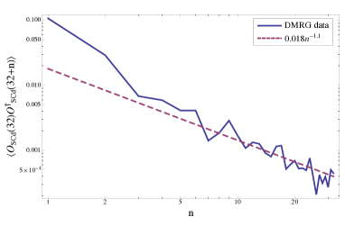
(b)

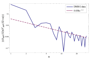
Figure 2: DMRG data (solid) and power law fits (dashed) for (a) the superconducting d-wave order parameter ${\cal O}_{SCd}$, and (b) the antibonding pairing order parameter ${\cal O}_{abP}$ on the $64\times 2$ ladder with $t=t_{\perp}=1$, $U=4$, $V_{\parallel}=V_{\perp}=0$ and $N=110$ electrons. Oscillations present in both two-point functions are contributions from sub-leading terms.

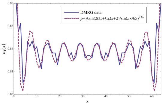
Figure 3: DMRG data (solid) and fit (dashed) for the one-point function of the density operator on leg $1$ of the the $64\times 2$ ladder with $t=t_{\perp}=1$, $U=4$, $V_{\parallel}=V_{\perp}=0$ and $N=110$ electrons. The fit function parameters take values $\rho=0.857$, $A=0.0054$ and $2K_{c}=0.91$. The bonding and antibonding wavevectors are given by $k_{b}=\rho_{b}\pi/2=1.17\pi/2$ and $k_{ab}=\rho_{ab}\pi/2=0.55\pi/2$, with $\rho_{b}$ ($\rho_{ab}$) the average density in the bonding (antibonding) band. The fit function takes the form discussed in Ref. Eggert09 for the $4k_{F}$ Wigner crystal oscillations. Additional oscillations arise from the sub-leading contributions of the charge density

V.2 $4k_{b}$ Umklapp

As is discussed in detail in Section III, there are two possible phases when the $4k_{b}$ Umklapp interaction is present and marginally relevant for the considered initial conditions. We consider in turn the $C1S2$ phase and the $C1S0$ phase which may occur as a result of the $4k_{b}$ Umklapp modifying the renormalization group equation. To that end we have carried out DMRG computations on the Hamiltonian

$$H=H_{\rm ladd}(\pi)+\mu_{-}\sum_{j,\sigma}\big{(}c^{\dagger}_{1,j,\sigma}-c^{\dagger}_{2,j,\sigma}\big{)}\big{(}c_{1,j,\sigma}-c_{2,j,\sigma}\big{)},$$ (78)

where $H_{\rm ladd}(K)$ is given by (1) and the bonding band is at quarter-filling. The additional term in (78) corresponds to a chemical potential for the antibonding pair and is introduced for convenience so that the antibonding density can be varied while keeping the interaction parameters constant. A quarter-filled bonding band requires an applied external potential of wavevector $4k_{b}=\pi$ to activate the $4k_{b}$ Umklapp interaction.

The reason for studying the model (78) rather than the doped ladder with quarter filled bonding band but without external potential is that in the latter both the Mott gap and spin gaps depend on the interaction strengths $U$, $V_{\parallel}$, $V_{\perp}$ and therefore cannot be tuned independently. As a result spin and charge gaps can be comparable in size and small, which makes a numerical analysis extremely challenging. In fact, our DMRG results for this case are inconclusive in the sense that we have not found convincing evidence for the existence of a C1S0 phase.

On the other hand, applying an external potential as in (78) allows us to control the Mott gap in the bonding sector without significantly affecting spin gaps. A sizeable Mott gap makes the numerical analysis much simpler.

V.2.1 $C1S2$ Phase

The RG analysis of section III shows that for sufficiently weak extended interactions (small $V_{\parallel},V_{\perp}$) the renormalization group flow of the extended Hubbard model in the presence of a $4k_{b}$ Umklapp interaction is towards a $C1S2$ fixed point. The two-point functions of the order parameters discussed in section III then have the following forms

$$\langle{\cal O}_{CDW}(x)\ {\cal O}^{\dagger}_{CDW}(0)\rangle_{C1S2} \propto {\cal A}_{3}\cos(2k_{ab}x){|x|^{-K_{2,c}-K_{2,s}}}+{\cal A}_{4}\cos(2k_{b}x)|x|^{-K_{1,s}}+{\cal A}_{5}x^{-2}+\ldots\ ,$$

$$\langle{\cal O}_{bCDW}(x)\ {\cal O}^{\dagger}_{bCDW}(0)\rangle_{C1S2} \propto e^{-|x|/\xi_{b}}\quad({\rm at~{}2}k_{b})+\ldots\ ,$$

$$\langle{\cal O}_{SCd}(x){\cal O}^{\dagger}_{SCd}(0)\rangle_{C1S2} \propto \cos(2k_{ab}x)|x|^{-K_{2,c}-1/K_{2,c}}+\ldots\ ,$$

$$\langle{\cal O}_{abP}(x){\cal O}^{\dagger}_{abP}(0)\rangle_{C1S2} \propto {\cal A}_{6}\cos(2k_{ab}x)|x|^{-K_{2,c}-1/K_{2,c}}+{\cal A}_{6}|x|^{-K_{2,s}-1/K_{2,c}}+\ldots,$$ (79)

where ${\cal A}_{j}$ are unknown amplitudes, $\xi_{b}$ is the bonding charge boson correlation length and $K_{2,c}$ ($K_{2,s}$) is the Luttinger parameter for antibonding charge (spin) sector.

In this section we present DMRG results for the $64\times 2$ extended-Hubbard ladder with $t=2t_{\perp}=1$, $U=8V_{\perp}=8V_{\parallel}=4$ and applied external potential of period $4k_{b}=\pi$ and amplitude $W_{1}=W_{2}=1.5$. The chemical potential $\mu_{-}$ has been adjusted so that the total electron number is $N=90$ with the bonding band at quarter-filling. Up to $m=1200$ density matrix states were kept in the simulations, leading to truncation errors of $\sim 10^{-6}$. This corresponds to a relative error in the ground state energy per site of $\epsilon\approx 10^{-4}$.

The presence of a charge gap in the bonding sector is confirmed by the examination of the Green’s functions in the bonding ($G_{b}(n)$) and antibonding ($G_{ab}(n))$ bands. The RG analysis suggests that $G_{ab}(n)$ decays as a power law, whereas $G_{b}(n)$ decreases with distance as an exponential multiplied by a power law.

The bonding Green’s function is shown in Fig. 4(a), where the leading oscillations at $k_{b}$ have been removed by performing a fit to the Green’s function and dividing out the oscillatory part. So, in Fig. 4(a) we plot

$$G_{b}(n)=\frac{G_{b,{\rm Full}}(n)}{\cos\left(k_{b}x\right)},$$

where $G_{b,{\rm Full}}(n)$ is the full bonding Green’s function with oscillations at $k_{b}$. The leading oscillation has been removed in order to elucidate the long-distance behaviour of the Green’s function. In this case the asymptotic behaviour is well described by an exponential multiplied by a power law, as predicted by the RG analysis. We perform a similar procedure for the antibonding Green’s function in Fig. 4(b), where the leading oscillations occur at $k_{ab}$. The power law decay of the antibonding Green’s function is in agreement with the RG analysis. The form of both Green’s functions is consistent with the expectations of the $C1S2$ phase, with a single massive charge boson in the bonding sector of the theory.

(a)

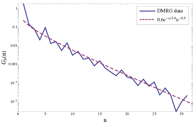
(b)

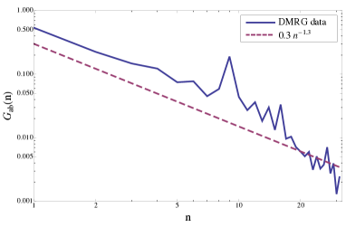
Figure 4: DMRG data (solid) and fits (dashed) for (a) the bonding Green’s function $G_{b}(n)=\langle c_{b}(32)c_{b}^{\dagger}(32+n)\rangle$ with $k_{b}$ oscillations removed (see text), and (b) the antibonding Green’s function $G_{ab}(n)=\langle c_{ab}(32)c_{ab}^{\dagger}(32+n)\rangle$ with $k_{ab}$ oscillations removed. Additional oscillations in both cases are due to sub-leading contributions of the Green’s functions. For both figures the $64\times 2$ ladder is considered with $t=2t_{\perp}=1$, $U=8V_{\perp}=8V_{\parallel}=4$ and $W_{+}=1.5$. The chemical potential $\mu_{-}$ was chosen such that the bonding band is quarter-filled for the system with $N=90$ electrons. Fit functions are of the form predicted by the RG analysis.

Having established the presence of a charge gap in the bonding sector, we now consider the two-point functions of the order parameters (79), shown in Fig. 5. As with our analysis of the Green’s function, the two-point functions of the antibonding pairing order parameter and the superconducting d-wave order parameter, shown in Fig. 5(a) and Fig. 5(b) respectively, have had the leading order $2k_{ab}$ oscillation removed. Both two-point functions show power law decay with the same exponent, giving an approximate value for the Luttinger parameter in the antibonding charge sector $K_{2,c}\approx 0.35$.

Figure 6 shows the two-point function of the charge density wave (CDW) order parameter. At intermediate distances this is well described by $x^{-2}$ decay, whilst for large distances it decays at slower-than-$x^{-2}$ and oscillates with wavenumber $2k_{ab}$, as predicted from the bosonization analysis (79). Sub-leading $4k_{b}$ contributions are also observed. The long-distance decay suggests that the Luttinger parameter in the antibonding spin sector is $K_{2,s}=1$, as expected from $SU(2)$ symmetry. The dominant correlations for considered parameters are of the charge density wave type.

(a)

(b)

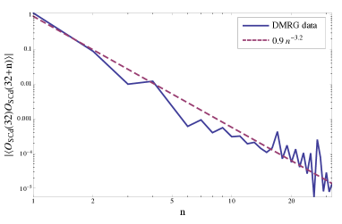
Figure 5: DMRG data (solid) and fit functions (dashed) for (a) the two-point function of the antibonding pairing order parameter ${\cal O}_{abP}$ with the $2k_{ab}$ oscillations removed (see text), and (b) the two-point function of the superconducting d-wave order parameter ${\cal O}_{SCd}$ with $2k_{ab}$ oscillations removed on the $64\times 2$ ladder with $t=2t_{\perp}=1$, $U=8V_{\perp}=8V_{\parallel}=4$ and $W_{+}=1.5$. The chemical potential has been adjusted so that $N=90$ coincides with a quarter-filled bonding band. Fit functions are of the form given in Eqs. (79).

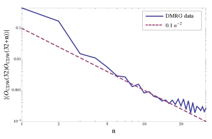
Figure 6: DMRG data (solid) and $x^{-2}$ guide (dashed) for the two-point function of the charge density wave order parameter ${\cal O}_{CDW}$ on the $64\times 2$ ladder with $t=2t_{\perp}=1$, $U=8V_{\perp}=8V_{\parallel}=4$ and $W_{+}=1.5$. The chemical potential has been adjusted so that $N=90$ coincides with a quarter-filled bonding band. Sub-$x^{-2}$ decay is observed with oscillations at $2k_{ab}$ at large distances.

V.2.2 $C1S0$ $4k_{b}$ Mott Insulator Phase

As has been discussed in Section III.1.2, in order for the $C1S0$ $4k_{b}$ Mott insulating phase to occur, it is necessary for the interchain exchange interaction to be antiferromagnetic after the initial renormalization group procedure. This can always be achieved provided the interchain density-density interaction coupling is large $V_{\perp}>U$, such that for the initial conditions the exchange interaction is antiferromagnetic and remains so under the renormalization group procedure.

At the $C1S0$ fixed point, the $4k_{b}$ Mott insulator phase is characterized by the following asymptotic forms of the two-point functions

$$\langle{\cal O}_{CDW}(x)\ {\cal O}^{\dagger}_{CDW}(0)\rangle \propto {\cal A}_{8}x^{-2}+{\cal A}_{9}\cos\big{(}2(k_{b}+k_{ab})x\big{)}|x|^{-K_{2,c}}+\ldots,$$

$$\langle{\cal O}_{bCDW}(x)\ {\cal O}^{\dagger}_{bCDW}(0)\rangle \propto e^{-|x|/\xi_{b}}~{}~{}({\rm at~{}2}k_{b})+\ldots,$$

$$\langle{\cal O}_{SCd}(x)\ {\cal O}^{\dagger}_{SCd}(0)\rangle \propto \cos(2k_{ab}x)|x|^{-K_{2,c}-1/K_{2,c}}+\ldots\ ,$$

$$\langle{\cal O}_{abP}(x)\ {\cal O}^{\dagger}_{abP}(0)\rangle \propto {\cal A}_{10}\cos(2k_{ab}x)|x|^{-K_{2,c}-1/K_{2,c}}+{\cal A}_{11}\cos\big{(}2k_{b}x\big{)}|x|^{-1/K_{2,c}}+\ldots\ ,$$ (80)

where ${\cal A}_{d}$ are unknown amplitudes.

We present results for the Hamiltonian (78) on on the $96\times 2$ ladder with $t=2t_{\perp}=1$, $V_{\perp}=5$, $V_{\parallel}=0$ and $U=4$. The chemical potential $\mu_{-}$ is used to set the total number of electrons to $N=88$ whilst maintaining the bonding band at quarter-filling. A periodic potential with period $4k_{b}=\pi$ and amplitude $W_{+}=1$ is applied to the bonding band. Up to $m=2000$ density matrix states were kept in the calculations, giving truncation errors of $\sim 10^{-7}$. The increased number of states in the procedure results in a relative error for the ground state energy per site of $\epsilon\approx 2\times 10^{-5}$.

The presence of a spin gap in both bands and a charge gap in the bonding band is inferred from the forms of the two-point functions (80) and the Green’s functions shown in Fig. 7. The RG analysis predicts that the bonding Green’s function should decay exponentially, whilst the antibonding Green’s function should decay as an exponential multiplied by a power law. In Fig. 7(a) the bonding Green’s function ($G_{b}(n)$) is shown with an exponential fit and is well described by exponential decay, implying both spin and charge gaps in the bonding sector. Figure 7(b) shows the antibonding Green’s function with with the leading oscillation at wavevector $k_{ab}$ removed in order to more clearly show the exponential multiplied by power law fit, as predicted by the RG analysis. The break in the plot of $G_{ab}(n)$ close to $n=28$ is a result of removing the oscillation; for this point the fit and $G_{ab}(n)$ differ in sign whilst both magnitudes are close to zero. The fit gives an approximate value for the Luttinger parameter in the antibonding charge sector $K_{2,c}\approx 0.27$.

With both Green’s functions being consistent with the $C1S0$ phase, the two-point functions of the order parameters in Eqs. (80) are now considered. The two-point functions for the SCd order parameter and the abP order parameter are presented in Fig. 8(a) and Fig. 8(b) respectively. In both cases the leading oscillation at frequency $2k_{ab}$ has been removed in order to elucidate the form of the decay, which in both cases is well described by a power law with an exponent consistent with $K_{2,c}\approx 0.27$. The absence of power law decay with exponent $1/K_{2,c}$ for the antibonding pairing order parameter is not inconsistent with being in the $C1S0$ phase, as the amplitude ${\cal A}_{11}$ is interaction-dependent and may be much smaller than the amplitude ${\cal A}_{10}$ of the sub-leading decay, in which case at short-distances the sub-leading decay would dominate.

The two-point function of the charge density wave order parameter is shown in Fig. 9. At long distances there are large wavelength oscillations with wavevector $2k_{b}+2k_{ab}$ decaying at sub-$x^{-2}$, consistent with the bosonization predictions for the $C1S0$ phase (80). The exact form of the decay of the $2k_{b}+2k_{ab}$ oscillations cannot be accurately extracted in the $L=96$ system, due to the large spin correlation length and the amplitudes ${\cal A}_{8}$ and ${\cal A}_{9}$ being unknown.

The two-point function of the bonding charge density wave order parameter can also be calculated, however information is not easily extracted from this two-point function due to the long spin correlation length and unknown interaction-induced amplitudes of $4k_{F}$ components of the bonding charge density operator, which are similar in form to those in Eqs. 95.

As discussed in detail in Section III.1.2, there are two possibilities for the dominant correlation in the $4k_{b}$ Mott insulator, depending upon $K_{2,c}$. For the presented case, $K_{2,c}<1$ and the dominant correlations are of charge density wave type, arising from the interaction-induced $2k_{b}+2k_{ab}$ component of the charge density.

(a)

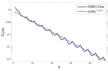
(b)

Figure 7: DMRG data (solid) and fit function (dashed) for (a) the bonding Green’s function $G_{b}(n)=\langle c_{b}(48)c_{b}^{\dagger}(48+n)\rangle$, and (b) the antibonding Green’s function $G_{ab}(n)=\langle c_{ab}(48)c_{ab}^{\dagger}(48+n)\rangle$, with the $k_{ab}$ oscillation removed (see text), for the $96\times 2$ ladder with $t=2t_{\perp}=1$, $U=4$, $V_{\parallel}=0$, $V_{y}=5$, $W_{+}=1$ and $N=88$ electrons. The chemical potential $\mu_{-}$ was chosen such that this corresponds to a quarter-filled bonding band. Oscillations in both plots are from other contributions to the Green’s function. The break in data of (b) at $n=29$ is a remnant of removing the $k_{ab}$ oscillations.

(a)

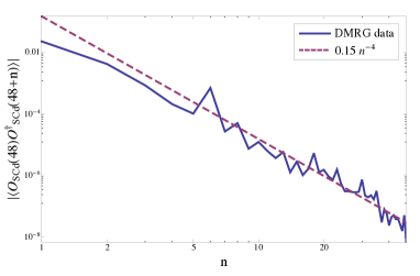
(b)

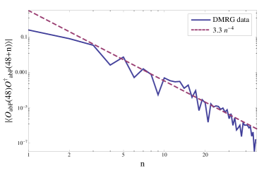
Figure 8: DMRG data (solid) and fit functions (dashed) for (a) the absolute value of the two-point function of the superconducting d-wave order parameter ${\cal O}_{SCd}$ with $2k_{ab}$ oscillations removed (see text), and (b) the absolute value of the two-point function of the antibonding pairing order parameter ${\cal O}_{abP}$ on the $96\times 2$ ladder with $t=2t_{\perp}=1$, $U=4$, $V_{\parallel}=0$, $V_{y}=5$, $W_{+}=1$ and $N=88$ electrons. The chemical potential $\mu_{-}$ was chosen such that this corresponds to a quarter-filled bonding band.

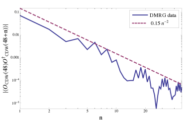
Figure 9: The two-point function of charge density wave order parameter ${\cal O}_{CDW}$ (solid) and $x^{-2}$ power law (dashed) for the $96\times 2$ ladder with $t=2t_{\perp}=1$, $U=4$, $V_{\perp}=5$ and $W_{+}=1$. A chemical potential applied to the antibonding band is used to set the electron number to $N=88$ with the bonding band quarter-filled.

VI Conclusions

In this work we have established a mechanism for finite wavevector pairing in doped fermionic ladders with equivalent legs. This mechanism is driven by Umklapp scattering processes, which occur either at special band fillings as a result of electron electron interactions, see also FradkinArx , or are induced by “externally” applied periodic potentials. The latter can arise via charge-density wave formation driven by the (three-dimensional) long-ranged Coulomb interaction in real crystal structures. We have applied renormalization group methods in the low-energy limit of the lattice model (1) for (i) weak interactions (”band representation”) and (ii) arbitrary interaction strength but very small tunneling along the rung direction (“chain representation”). In both cases we have found that the theory describing the strong coupling fixed point is the same as the low energy description of the so-called Kondo-Heisenberg Model (KHM) zachar ; berg . In the case of the $4k_{b}$ Mott insulator analyzed in section III this fact may be anticipated on the basis of the following arguments. The $4k_{b}$ Umklapp scattering process leads to formation of a Mott gap $\Delta$ within the bonding band. At low-energies the charge dynamics is the blocked by the Mott gap and at energies small compared to $\Delta$ one is left with spin degrees of freedom, that can be thought of in terms of an effective spin-1/2 Heisenberg chain. The antibonding degrees of freedom remain gapless, and at low energies compared to $\Delta$ the most important interaction with the bonding degrees of freedom is then through an effective spin exchange interaction. The resulting picture is an effective KHM, where the spin-1/2 chain corresponds to the bonding band and the role of the interacting 1D electron gas is played by the antibonding band. The low energy limit is crucial for these considerations to hold, because in the lattice model (1) electron number in the bonding band is not conserved.

Another important difference between the effective KHM that emerges as the low-energy description of the ladder and the lattice KHM model considered in zachar ; berg is that the effective exchange interaction between the bonding and antibonding bands is not a priori antiferromagnetic. In the case of weakly interacting Hubbard chains it is in fact ferromagnetic, which results in a C1S2 phase as the exchange interaction is marginally irrelevant. On the other hand, we found that extended density-density interactions (we explicitly consider repulsive nearest-neighbor interactions) can cause this exchange interaction to become antiferromagnetic. In this case the low-energy sector of the theory is a C1S0 phase, where the remaining gapless degree of freedom describes the antibonding charge sector and is characterized by its Luttinger parameter $K_{2,c}$. The dominant correlations are then either of superconducting PDW (if $K_{2,c}>1$) or CDW (if $K_{2,c}<1$) type.

The activation of the Umklapp scattering process at $3k_{b}+k_{ab}$ results in a similar low-energy description, although here the remaining massless degree of freedom $\tilde{\Phi}_{2}$ is significantly more complicated: it is a combination of the symmetric charge boson $\Phi_{c}$ and the U(1) doublet Majorana fermions $\xi^{1,2}$, which are themselves comprised of the SU(2) singlet Majorana fermion from the antisymmetric spin sector and a Majorana fermion from the antisymmetric charge sector. The composite nature of this gapless degree of freedom makes the analysis of ground state correlations difficult and we leave this issue to future studies.

Appendix A The Charge Density Operator

At commensurate fillings, or by applying an appropriate external periodic potential, Umklapp scattering processes can be activated in the doped ladder. In this case, oscillatory components of the charge density which are usually suppressed away from commensurate fillings now feature in the Hamiltonian. In this appendix we consider the $2k_{F}$ and $4k_{F}$ harmonics of the charge density operator in the “band” and “chain” representations in turn.

A.1 $2k_{F}$ Components of the Charge Density

We first consider the $2k_{F}$ harmonics in the “band” representation. The number operators on each leg of the ladder can be expressed in terms of the bonding/antibonding fermions introduced in (3) as

$$n_{1,j,\alpha}+n_{2,j,\alpha} = c^{\dagger}_{b,j,\alpha}c_{b,j,\alpha}+c^{\dagger}_{ab,j,\alpha}c_{ab,j,\alpha}\ ,$$

$$n_{1,j,\alpha}-n_{2,j,\alpha} = c^{\dagger}_{b,j,\alpha}c_{ab,j,\alpha}+c^{\dagger}_{ab,j,\alpha}c_{b,j,\alpha}\ .$$ (81)

Linearizing about the Fermi surface and taking the continuum limit as in (6), we obtain the following decompositions

$$n_{1,j,\alpha}+n_{2,j,\alpha} \sim a_{0}\rho^{(+)}_{0,\alpha}(x)+a_{0}\left[\rho^{(+)}_{2k_{b},\alpha}(x)\ e^{2ik_{b}x}+\rho^{(+)}_{2k_{ab},\alpha}(x)\ e^{2ik_{b}x}+{\rm h.c.}\right]+\ldots\ ,$$

$$n_{1,j,\alpha}-n_{2,j,\alpha} \sim a_{0}\left[\rho^{(-)}_{k_{b}+k_{ab},\alpha}(x)\ e^{i(k_{b}+k_{ab})x}+{\rm h.c.}\right]+\ldots,$$ (82)

where

$$\rho^{(+)}_{0,\alpha}(x) = R^{\dagger}_{b,\alpha}R_{b,\alpha}+L^{\dagger}_{b,\alpha}L_{b,\alpha}+R^{\dagger}_{ab,\alpha}R_{ab,\alpha}+L^{\dagger}_{ab,\alpha}L_{ab,\alpha}\ ,$$

$$\rho^{(+)}_{2k_{b},\alpha}(x) = L^{\dagger}_{b,\alpha}R_{b,\alpha}\ ,\ \rho^{(+)}_{2k_{ab},\alpha}(x)=L^{\dagger}_{ab,\alpha}R_{ab,\alpha}\ ,$$

$$\rho^{(-)}_{k_{b}+k_{ab},\alpha}(x) = L^{\dagger}_{ab,\alpha}R_{b,\alpha}+L^{\dagger}_{b,\alpha}R_{ab,\alpha}\ .$$ (83)

We note that $\rho_{0,\alpha}(x)$, $\rho_{2k_{b},\alpha}(x)$ and $\rho_{2k_{ab},\alpha}(x)$ are even under interchange of legs 1 and 2 of the ladder, while $\rho_{k_{b}+k_{ab},\alpha}(x)$ is odd. The components can then be bosonized following GNT and (11-13). This leads to the following expressions for components of the charge density operator

$$\rho^{(+)}_{0}(x) = \sum_{\alpha}\rho^{(+)}_{0,\alpha}(x)\sim\frac{1}{\sqrt{2\pi}}\partial_{x}\Phi_{+c}\ ,$$

$$\rho^{(+)}_{2k_{b}}(x) = \sum_{\alpha}\rho^{(+)}_{2k_{b},\alpha}(x)\sim-2i\ e^{i\sqrt{\pi}(\Phi_{+,c}+\Phi_{-,c})}\cos\Big{[}\sqrt{\pi}(\Phi_{+,s}+\Phi_{-,s})\Big{]}\ ,$$

$$\rho^{(+)}_{2k_{ab}}(x) = \sum_{\alpha}\rho^{(+)}_{2k_{ab},\alpha}(x)\sim-2i\ e^{i\sqrt{\pi}(\Phi_{+,c}-\Phi_{-,c})}\cos\Big{[}\sqrt{\pi}(\Phi_{+,s}-\Phi_{-,s})\Big{]}\ ,$$

$$\rho^{(-)}_{k_{b}+k_{ab}}(x) \sim -2i\ e^{i\sqrt{\pi}\Phi_{+,c}}\Big{[}e^{-i\sqrt{\pi}\Theta_{-,c}}\cos\left(\sqrt{\pi}[\Phi_{+,s}-\Theta_{-,s}]\right)-e^{i\sqrt{\pi}\Theta_{-,c}}\cos\left(\sqrt{\pi}[\Phi_{+,s}+\Theta_{-,s}]\right)\Big{]},$$ (84)

where $\Phi_{\pm,d}=(\Phi_{1,d}\pm\Phi_{2,d})/\sqrt{2}$ and $\Theta_{\pm,d}=(\Theta_{1,d}\pm\Theta_{2,d})/\sqrt{2}$ for $d=c,s$. In the final term we have used that $\kappa_{b,\uparrow}\kappa_{ab,\uparrow}\equiv\kappa_{b,\downarrow}\kappa_{ab,\downarrow}$ and $(\kappa_{b,\sigma}\kappa_{ab,\sigma})^{2}=-1$. Here we note that the $2k_{F}$ response of the charge density in spin gapped phases is blocked as each term features a spin boson.

Having moved to a new basis of bosons, the $\pm$ bosons, we can consider refermionizing the spin bosons and the antisymmetric charge bosons using the using the identities GNT

$$e^{i\sqrt{\pi}\Phi_{+,s}} \sim \mu_{1}\mu_{2}+i\sigma_{1}\sigma_{2}\ ,\qquad e^{i\sqrt{\pi}\Theta_{+,s}}\sim\sigma_{1}\mu_{2}+i\mu_{1}\sigma_{2}\ ,$$

$$e^{i\sqrt{\pi}\Phi_{-,s}} \sim \mu_{3}\mu_{4}+i\sigma_{3}\sigma_{4}\ ,\qquad e^{i\sqrt{\pi}\Theta_{-,s}}\sim\sigma_{3}\mu_{4}+i\mu_{3}\sigma_{4}\ ,$$

$$e^{i\sqrt{\pi}\Phi_{-,c}} \sim \mu_{5}\mu_{6}+i\sigma_{5}\sigma_{6}\ ,\qquad e^{i\sqrt{\pi}\Theta_{-,c}}\sim\sigma_{5}\mu_{6}+i\mu_{5}\sigma_{6}\ ,$$ (85)

where $\mu_{i}$ and $\sigma_{i}$ are Majorana fermions. Then the $2k_{F}$ components of the charge density operator can be expressed in terms of the Majorana fermions as

$$\rho^{(+)}_{2k_{b}}(x) \propto -2i\ e^{i\sqrt{\pi}\Phi_{+,c}}\left[\mu_{5}\mu_{6}+i\sigma_{5}\sigma_{6}\right]\left[\mu_{1}\mu_{2}\mu_{3}\mu_{4}-\sigma_{1}\sigma_{2}\sigma_{3}\sigma_{4}\right]\ ,$$

$$\rho^{(+)}_{2k_{ab}}(x) \propto -2i\ e^{i\sqrt{\pi}\Phi_{+,c}}\left[\mu_{5}\mu_{6}-i\sigma_{5}\sigma_{6}\right]\left[\mu_{1}\mu_{2}\mu_{3}\mu_{4}+\sigma_{1}\sigma_{2}\sigma_{3}\sigma_{4}\right]\ ,$$

$$\rho^{(-)}_{k_{b}+k_{ab}}(x) \propto -4i\ e^{i\sqrt{\pi}\Phi_{+,c}}\left[\sigma_{1}\sigma_{2}\mu_{3}\sigma_{4}\sigma_{5}\mu_{6}-i\mu_{1}\mu_{2}\sigma_{3}\mu_{4}\mu_{5}\sigma_{6}\right]\ .$$

Similar expressions are obtained in the chain description with leg indices substituted for band indices.

Appendix B $4k_{F}$ Density Components in the Band Picture

To derive the $4k_{F}$-components of the charge density, we consider the on-site Hubbard interaction

$$U\sum_{m=1}^{L}[n_{1,m,\uparrow}n_{1,m,\downarrow}+n_{2,m,\uparrow}n_{2,m,\downarrow}]\ ,$$ (86)

which gives a contribution $S_{\rm int}=S_{\rm int}^{(1)}+S_{\rm int}^{(2)}$ to the action

$$S_{\rm int}^{(1)} = -\frac{U}{2}\int d^{2}{\bf y}\left[c^{\dagger}_{b,\uparrow}c_{b,\uparrow}+c^{\dagger}_{ab,\uparrow}c_{ab,\uparrow}\right]({\bf y})\left[c^{\dagger}_{b,\downarrow}c_{b,\downarrow}+c^{\dagger}_{ab,\downarrow}c_{ab,\downarrow}\right]({\bf y})$$

$$S_{\rm int}^{(2)} = -\frac{U}{2}\int d^{2}{\bf y}\left[c^{\dagger}_{b,\uparrow}c_{ab,\uparrow}+c^{\dagger}_{ab,\uparrow}c_{b,\uparrow}\right]({\bf y})\left[c^{\dagger}_{b,\downarrow}c_{ab,\downarrow}+c^{\dagger}_{ab,\downarrow}c_{b,\downarrow}\right]({\bf y})\ .$$ (87)

We then decompose the continuum fields into their high and low-energy parts, e.g.

$$c_{b}(x)=c_{b,<}(x)+c_{b,>}(x)\ .$$ (88)

The $4k_{F}$ components of the charge density are then found by taking the average

$$-\Big{\langle}c^{\dagger}_{b}(x)c_{b}(x)S_{\rm int}\Big{\rangle}_{>}$$ (89)

over the high-energy degrees of freedom and keep only the $4k_{F}$ oscillating parts. For example, we obtain a contribution

$$\frac{U}{2}\Big{\langle}c^{\dagger}_{b,\uparrow,<}(x)c_{b,\uparrow,>}(x)\int dyd\tau\ c^{\dagger}_{b,\uparrow,>}c_{b,\uparrow,<}\left[c^{\dagger}_{b,\downarrow,<}c_{b,\downarrow,<}+c^{\dagger}_{ab,\downarrow,<}c_{ab,\downarrow,<}\right]\Big{\rangle}_{>},$$ (90)

where we now use that

$$\big{\langle}c_{b,\uparrow,>}(x)\ c^{\dagger}_{b,\uparrow,>}(\tau,y)\big{\rangle}=G_{b,>}(-\tau,x-y)=-\int_{k>\Lambda}\frac{dk}{2\pi}\ e^{-ik(x-y)-\epsilon_{b}(k)\tau}$$ (91)

is short ranged in $\tau$, so it becomes

$$\frac{U}{2}c^{\dagger}_{b,\uparrow,<}(x)\int d\tau dy\ G_{b,>}(-\tau,x-y)c_{b,\uparrow,<}(y)\left[c^{\dagger}_{b,\downarrow,<}c_{b,\downarrow,<}+c^{\dagger}_{ab,\downarrow,<}c_{ab,\downarrow,<}\right](y).$$ (92)

Next we linearize about the Fermi surface, which decomposes the fermion operators into their chiral components

$$c_{b,\uparrow,<}(y)\simeq R_{b,\uparrow}e^{ik_{b}y}+L_{b,\uparrow}e^{-ik_{b}y}$$ (93)

and then we replace the arguments of the left and right moving fermions by $x$, which is justified as the Green’s function is also short-ranged in $x-y$. Implementation of this procedure leads to the following results for the $4k_{F}$-components of the charge density

$$\rho^{(+)}_{4k_{b}}(x) \sim {U}G_{b,>}(3k_{b})\sum_{\alpha=\uparrow,\downarrow}L^{\dagger}_{b,\alpha}R_{b,\alpha}L^{\dagger}_{b,-\alpha}R_{b,-\alpha}\ ,$$

$$\rho^{(+)}_{4k_{ab}}(x) \sim {U}G_{ab,>}(3k_{ab})\sum_{\alpha=\uparrow,\downarrow}L^{\dagger}_{ab,\alpha}R_{ab,\alpha}L^{\dagger}_{ab,-\alpha}R_{ab,-\alpha}\ ,$$

$$\rho^{(+)}_{2k_{b}+2k_{ab}}(x) \sim \frac{U}{2}\big{[}G_{b,>}(k_{ab}+2k_{b})+G_{b,>}(k_{b}+2k_{ab})\big{]}\sum_{\alpha=\uparrow,\downarrow}\Big{\{}2L^{\dagger}_{b,\alpha}R_{b,\alpha}L^{\dagger}_{ab,-\alpha}R_{ab,-\alpha}$$

$$+2L^{\dagger}_{b,\alpha}R_{ab,\alpha}L^{\dagger}_{ab,-\alpha}R_{b,-\alpha}+L^{\dagger}_{b,\alpha}R_{ab,\alpha}L^{\dagger}_{b,-\alpha}R_{ab,-\alpha}+L^{\dagger}_{ab,\alpha}R_{b,\alpha}L^{\dagger}_{ab,-\alpha}R_{b,-\alpha}\Big{\}}\ ,$$

$$\rho^{(-)}_{k_{b}+3k_{ab}}(x) \sim \frac{U}{2}\big{[}3G_{b,>}(k_{ab}+2k_{b})+G_{ab,>}(3k_{ab})\big{]}\sum_{\alpha=\uparrow,\downarrow}\Big{\{}L^{\dagger}_{ab,\alpha}R_{ab,\alpha}L^{\dagger}_{ab,-\alpha}R_{b,-\alpha}+L^{\dagger}_{ab,\alpha}R_{ab,\alpha}L^{\dagger}_{b,-\alpha}R_{ab,-\alpha}\Big{\}}\ ,$$

$$\rho^{(-)}_{3k_{b}+k_{ab}}(x) \sim \frac{U}{2}\big{[}3G_{ab,>}(k_{ab}+2k_{b})+G_{b,>}(3k_{b})\big{]}\sum_{\alpha=\uparrow,\downarrow}\Big{\{}L^{\dagger}_{b,\alpha}R_{b,\alpha}L^{\dagger}_{b,-\alpha}R_{ab,-\alpha}+L^{\dagger}_{b,\alpha}R_{b,\alpha}L^{\dagger}_{ab,-\alpha}R_{b,-\alpha}\Big{\}}\ .$$ (94)

These expressions can be bosonized following Ref. GNT , giving

$$\rho^{(+)}_{4k_{b}}(x) \sim -2UG_{b,>}(3k_{b})\ e^{i\sqrt{4\pi}\Phi_{+,c}}\ e^{i\sqrt{4\pi}\Phi_{-,c}}\ ,$$

$$\rho^{(+)}_{4k_{ab}}(x) \sim -2UG_{ab,>}(3k_{ab})\ e^{i\sqrt{4\pi}\Phi_{+,c}}\ e^{-i\sqrt{4\pi}\Phi_{-,c}}\ ,$$

$$\rho^{(+)}_{2k_{b}+2k_{ab}}(x) \sim {\cal C}_{2k_{b}+2k_{ab}}\ e^{i\sqrt{4\pi}\Phi_{+,c}}\left[\cos\big{(}\sqrt{4\pi}\Phi_{-,s}\big{)}+\cos\big{(}\sqrt{4\pi}\Theta_{-,s}\big{)}-\cos\big{(}\sqrt{4\pi}\Theta_{-,c}\big{)}\right]\ ,$$

$$\rho^{(-)}_{3k_{b}+k_{ab}}(x) \sim {\cal C}_{3k_{b}+k_{ab}}e^{i\sqrt{4\pi}\Phi_{+,c}}\left[e^{-i\sqrt{\pi}\bar{\varphi}_{-,c}}\cos(\sqrt{\pi}\varphi_{-,s})-e^{i\sqrt{\pi}{\varphi}_{-,c}}\cos(\sqrt{\pi}\bar{\varphi}_{-,s})\right]\ ,$$

$$\rho^{(-)}_{k_{b}+3k_{ab}}(x) \sim {\cal C}_{k_{b}+3k_{ab}}e^{i\sqrt{4\pi}\Phi_{+,c}}\left[e^{-i\sqrt{\pi}{\varphi}_{-,c}}\cos(\sqrt{\pi}\bar{\varphi}_{-,s})-e^{i\sqrt{\pi}{\bar{\varphi}}_{-,c}}\cos(\sqrt{\pi}{\varphi}_{-,s})\right]\ ,$$ (95)

where ${\cal C}_{p}$ are non-universal prefactors that are proportional to $U$ for small interactions and the fields $\varphi_{\pm,d}$ and $\bar{\varphi}_{\pm,d}$ are chiral components of the boson field $\Phi_{\pm,d}$ for $d=c,s$ which satisfy

$$\Phi_{\pm,d} = \varphi_{\pm,d}+\bar{\varphi}_{\pm,d}\ ,$$

$$\Theta_{\pm,d} = \varphi_{\pm,d}-\bar{\varphi}_{\pm,d}\ .$$

Once more we may refermionize Eqs. (95) in terms of the new basis of bosons, i.e.

$$R_{1}+iR_{2} \sim \frac{\kappa_{+,s}}{\sqrt{\pi a_{0}}}e^{i\sqrt{4\pi}\varphi_{+,s}},\quad L_{1}+iL_{2}\sim\frac{\kappa_{+,s}}{\sqrt{\pi a_{0}}}e^{-i\sqrt{4\pi}\bar{\varphi}_{+,s}}\ ,$$

$$R_{3}+iR_{4} \sim \frac{\kappa_{-,s}}{\sqrt{\pi a_{0}}}e^{i\sqrt{4\pi}\varphi_{-,s}},\quad L_{3}+iL_{4}\sim\frac{\kappa_{-,s}}{\sqrt{\pi a_{0}}}e^{-i\sqrt{4\pi}\bar{\varphi}_{-,s}}\ ,$$

$$R_{5}+iR_{6} \sim \frac{\kappa_{-,c}}{\sqrt{\pi a_{0}}}e^{i\sqrt{4\pi}\varphi_{-,c}},\quad L_{5}+iL_{6}\sim\frac{\kappa_{-,c}}{\sqrt{\pi a_{0}}}e^{-i\sqrt{4\pi}\bar{\varphi}_{-,c}}\ ,$$ (96)

where $\kappa$ are Klein factors introduced to ensure that different Majoranas anticommute. This choice of basis for the Majorana fermions will make the “dictionary” (30) between the “band” representation and the “chain” representation particularly clear. The $4k_{F}$ components of the charge density are local with respect to the Majoranas

$$\rho^{(+)}_{4k_{b}}(x) \propto e^{i\sqrt{4\pi}\Phi_{+,c}}\ \left[R_{5}L_{6}-R_{6}L_{5}+i(R_{5}L_{5}+R_{6}L_{6})\right]\ ,$$

$$\rho^{(+)}_{4k_{ab}}(x) \propto e^{i\sqrt{4\pi}\Phi_{+,c}}\ \left[R_{5}L_{6}-R_{6}L_{5}-i(R_{5}L_{5}+R_{6}L_{6})\right]\ ,$$

$$\rho^{(+)}_{2k_{b}+2k_{ab}}(x) \propto e^{i\sqrt{4\pi}\Phi_{+,c}}\ i\left[2R_{4}L_{4}+R_{5}L_{5}-R_{6}L_{6}\right]\ ,$$

$$\rho^{(-)}_{3k_{b}+k_{ab}}(x) \propto e^{i\sqrt{4\pi}\Phi_{+,c}}\left[(L_{5}+iL_{6})R_{3}-(R_{5}+iR_{6})L_{3}\right]\,,$$

$$\rho^{(-)}_{k_{b}+3k_{ab}}(x) \propto e^{i\sqrt{4\pi}\Phi_{+,c}}\left[(R_{5}-iR_{6})L_{3}-(L_{5}-iL_{6})R_{3}\right]\ .$$ (97)

B.1 “$4k_{F}$” Density Components in the Chain Picture

In this Appendix we determine the Fourier components with momenta close to $4k_{F}$ of the low-energy projections of $n_{1,l}\pm n_{2,l}$, c.f. eqn (2), in the chain picture. For uncoupled chains we have

$$n_{1,l}\pm n_{2,l}\Big{|}_{t_{\perp}=0}\propto\sum_{n\in\mathbb{Z}}\widetilde{\rho}^{(\pm)}_{2nk_{F}}(x)e^{2ink_{F}x}.$$ (98)

For non-zero $t_{\perp}$ this expressions gets modified to

$$n_{1,l}\pm n_{2,l}\propto\sum_{P\in S_{\pm}}{\rho}^{(\pm)}_{P}(x)e^{iPx},$$ (99)

where $S_{\pm}$ are appropriately defined sets of momenta. Our starting point is the bosonized expression for the $4k_{F}$ components of the charge density of the extended Hubbard chains describing the uncoupled legs $\ell=1,2$ of the ladder (i.e. $t_{\perp}=0=V_{\perp}=W_{1,2}$)

$$\rho_{4k_{F}}^{(\ell)}(x)\sim\tilde{F}e^{i4k_{F}x}e^{i\sqrt{8\pi}\Phi^{(c)}_{\ell}}+\mathrm{h.c.}\ ,$$ (100)

where $\tilde{F}$ is a non-universal amplitude. The sum of the $4k_{F}$ densities of the two legs can be expressed in terms of the rotated boson basis (16) as

$$\widetilde{\rho}^{(+)}_{4k_{F}}(x)\sim 2\tilde{F}\cos(4k_{F}x+\sqrt{4\pi}\Phi_{c})\cos(\sqrt{4\pi}\Phi_{f}).$$ (101)

We will now take into account the effects of a nonzero $t_{\perp}$ by following through the same steps as in the analysis of the Hamiltonian in section II.2. Refermionizing in terms of Majorana fermions using the identities

$$\tilde{\kappa}e^{i\sqrt{\pi}\big{(}\Phi_{f}+\Theta_{f}\big{)}} = \sqrt{\pi a_{0}}\left(\xi_{R}^{3}+i\eta_{R}\right),$$

$$\tilde{\kappa}e^{-i\sqrt{\pi}\big{(}\Phi_{f}+\Theta_{f}\big{)}} = \sqrt{\pi a_{0}}\left(\xi_{L}^{3}+i\eta_{L}\right),$$ (102)

where $\tilde{\kappa}$ is a Klein factor and $\tilde{\kappa}^{2}=1$ leads to

$$\cos(\sqrt{4\pi}\Phi_{f})=i\pi a_{0}\left(\xi_{R}^{3}\xi_{L}^{3}+\eta_{R}\eta_{L}\right).$$ (103)

Finally, performing the rotation (II.2) we arrive at

$$\cos(\sqrt{4\pi}\Phi_{f}) \approx i\pi a_{0}\Bigg{\{}\xi_{R}^{3}\xi_{L}^{3}+\frac{v_{s}}{v_{s}+v_{c}}\Big{[}\xi_{R}^{1}\xi^{1}_{L}-\xi_{R}^{2}\xi_{L}^{2}-\frac{1}{2}e^{2iQx}\left(\xi_{R}^{1}-i\xi_{R}^{2}\right)\left(\xi_{L}^{1}+i\xi_{L}^{2}\right)$$ (104)

$$\qquad\qquad\qquad-\frac{1}{2}e^{-2iQx}\left(\xi_{R}^{1}+i\xi_{R}^{2}\right)\left(\xi_{L}^{1}-i\xi_{L}^{2}\right)\Big{]}\Bigg{\}}.$$

Substituting (104) into (101) then gives us expressions for the Fourier components of the total symmetric charge density of the ladder for non-zero $t_{\perp}$

$$\rho^{(+)}_{4k_{F}}(x) \sim iFe^{i\sqrt{4\pi}\Phi_{c}}\left[\xi_{R}^{3}\xi_{L}^{3}+\frac{v_{s}}{v_{s}+v_{c}}\left(\xi_{R}^{1}\xi_{L}^{1}-\xi_{R}^{2}\xi_{L}^{2}\right)\right],$$

$$\rho^{(+)}_{4k_{F}+2Q}(x) \sim \frac{iFv_{s}}{2\left(v_{s}+v_{c}\right)}e^{i\sqrt{4\pi}\Phi_{c}}\left(\xi_{L}^{1}+i\xi_{L}^{2}\right)\left(\xi_{R}^{1}-i\xi_{R}^{2}\right),$$

$$\rho^{(+)}_{4k_{F}-2Q}(x) \sim \frac{iFv_{s}}{2\left(v_{s}+v_{c}\right)}e^{i\sqrt{4\pi}\Phi_{c}}\left(\xi_{L}^{1}-i\xi_{L}^{2}\right)\left(\xi_{R}^{1}+i\xi_{R}^{2}\right),$$

and $F=\tilde{F}\pi a_{0}$ is a non-universal constant. The analogous analysis for the antisymmetric combination of charge densities gives the following result

$$\rho^{(-)}_{4k_{F}-Q}(x) = -iF\sqrt{\frac{v_{s}}{2\left(v_{s}+v_{c}\right)}}e^{i\sqrt{4\pi}\Phi_{c}}\left[\left(\xi_{R}^{1}+i\xi_{R}^{2}\right)\xi_{L}^{3}+\xi_{R}^{3}\left(\xi_{L}^{1}-i\xi_{L}^{2}\right)\right]\ ,$$ (105)

$$\rho^{(-)}_{4k_{F}+Q}(x) = -iF\sqrt{\frac{v_{s}}{2\left(v_{s}+v_{c}\right)}}e^{i\sqrt{4\pi}\Phi_{c}}\left[\left(\xi_{R}^{1}-i\xi_{R}^{2}\right)\xi_{L}^{3}+\xi_{R}^{3}\left(\xi_{L}^{1}+i\xi_{L}^{2}\right)\right]\ ,$$ (106)

where $F$ is the same non-universal constant as in the $(+)$ component case.

Appendix C Higher Harmonics of the Bond-Centered Antibonding Superconducting Order Parameter

We consider the order parameter for bond-centered pairing in the antibonding band:

$$\Phi_{B}(j)=c_{ab,\uparrow}(j)c_{ab,\downarrow}(j+1)-c_{ab,\downarrow}(j)c_{ab,\uparrow}(j+1)$$

and consider the higher-order term generated by the four-fermion interaction. We integrate out the high-energy part of the Hubbard interaction (87) by splitting the fermion operators into fast (high-energy $>$) and slow (low-energy $<$) components as shown in (88). We separate the “mixed” part of the bond-centered pairing order parameter into four contributions

$${\cal O}_{1} = c_{ab,\uparrow,>}(x)c_{ab,\downarrow,<}(x+a_{0}),\qquad\qquad{\cal O}_{3}=c_{ab,\uparrow,<}(x)c_{ab,\downarrow,>}(x+a_{0}),$$

$${\cal O}_{2} = -c_{ab,\downarrow,>}(x)c_{ab,\uparrow,<}(x+a_{0}),\qquad\quad~{}{\cal O}_{4}=-c_{ab,\downarrow,<}(x)c_{ab,\uparrow,>}(x+a_{0}).$$ (107)

We now discuss in some detail the perturbative averaging of the operator ${\cal O}_{1}$ with respect to the interaction term $S_{\rm int}^{(1)}$. We have

$$\langle{\cal O}_{1}S_{\rm int}^{(1)}\rangle_{>} = -\frac{U}{2}\int{\rm d}^{2}{\bf y}~{}\Biggl{\langle}c_{ab,\uparrow,>}(x)c_{ab,\downarrow,<}(x+a_{0})$$

$$\times \left[c_{ab,\uparrow,<}^{\dagger}c_{ab,\uparrow,<}+c_{ab.\uparrow,<}^{\dagger}c_{ab,\uparrow,>}+c_{ab,\uparrow,>}^{\dagger}c_{ab,\uparrow,<}+c_{ab,\uparrow,>}^{\dagger}c_{ab,\uparrow,>}+b\leftrightarrow ab\right]({\bf y})$$

$$\times \left[c_{ab,\downarrow,<}^{\dagger}c_{ab,\downarrow,<}+c_{ab.\downarrow,<}^{\dagger}c_{ab,\downarrow,>}+c_{ab,\downarrow,>}^{\dagger}c_{ab,\downarrow,<}+c_{ab,\downarrow,>}^{\dagger}c_{ab,\downarrow,>}+b\leftrightarrow ab\right]({\bf y})\Biggr{\rangle}_{>}.$$

This can now be averaged over the high-energy parts and the resulting expression evaluated in the continuum limit by following the same steps as in Appendix B. We then bosonize, following GNT , and the result is

$$\langle{\cal O}_{1}S_{\rm int}^{(1)}\rangle_{>}\sim\frac{U}{2}\frac{\kappa_{ab,\downarrow}\kappa_{ab,\uparrow}}{(2\pi)^{2}}ie^{i\sqrt{2\pi}\Theta_{2,c}} \Bigg{\{} G_{ab,\uparrow,-}\cos\left(\sqrt{2\pi}\Phi_{1,c}+2k_{b}x\right)\cos\left(\sqrt{4\pi}\Phi_{+,s}-k_{ab}a_{0}\right)+$$ (108)

$$G_{ab,\uparrow,-}\sin\left(\sqrt{2\pi}\Phi_{1,c}+2k_{b}x\right)\sin\left(\sqrt{4\pi}\Phi_{+,s}-k_{ab}a_{0}\right)+$$

$$iG_{ab,\uparrow,+}\sin\left(\sqrt{2\pi}\Phi_{1,c}+2k_{b}x\right)\cos\left(\sqrt{4\pi}\Phi_{+,s}-k_{ab}a_{0}\right)-$$

$$iG_{ab,\uparrow,+}\cos\left(\sqrt{2\pi}\Phi_{1,c}+2k_{b}x\right)\sin\left(\sqrt{4\pi}\Phi_{+,s}-k_{ab}a_{0}\right)\Bigg{\}}$$

where $G_{ab,\uparrow,\pm}=G_{ab,\uparrow}(2k_{b}-k_{ab})\pm G_{ab,\uparrow}(k_{ab}-2k_{b})$. There terms arise from the four-fermion products

$$R_{ab,\downarrow}(x+a_{0})L_{ab,\uparrow}(x)L_{b,\downarrow}^{\dagger}(x)R_{b,\downarrow}(x)\qquad\qquad L_{ab,\downarrow}(x+a_{0})R_{ab,\uparrow}(x)R_{b\downarrow}^{\dagger}(x)L_{b,\downarrow}(x)\ .$$

These describe the coupling of “$2k_{b}$” density oscillations in the bonding band to bond-centered hole pairs in the antibonding band. Carrying out the analogous analyses for ${\cal O}_{2}$, ${\cal O}_{3}$ and ${\cal O}_{4}$ we find the sum of the contributions is given by

$$\langle\Phi_{B}S_{\rm int}^{(1)}\rangle\sim e^{i\sqrt{2\pi}\Theta_{2,c}} \Big{[}{\cal C}_{1}\cos\left(\sqrt{2\pi}\Phi_{1,c}+2k_{b}x\right)+{\cal C}_{2}\sin\left(\sqrt{2\pi}\Phi_{1,c}+2k_{b}x\right)\Big{]}\cos\left(\sqrt{4\pi}\Phi_{+,s}\right)+\ldots\ ,$$ (109)

where the complex coefficients ${\cal C}_{1,2}$ are given in terms of $G_{ab,\uparrow,\pm}$ and where we have retained only the terms which contribute power-law decay to the two point function. Terms which have zero expectation value in the $4k_{b}$ Mott insulator, e.g. contributions proportional to $\sin(\sqrt{4\pi}\Phi_{+,s})$ or $\sin(\sqrt{4\pi}\Theta_{-,s})$, have been dropped from (109). The order parameter $\Phi_{B}$ being bond-centered is important; the contributions (109) which decay as a power law in the $4k_{b}$ Mott insulating phase vanish due to cancellation in the site-centered case. Following through the same steps for $S_{\rm int}^{(2)}$ we find that

$$\langle\Phi_{B}S_{\rm int}^{(2)}\rangle \sim -e^{i\sqrt{2\pi}\Theta_{2,c}}\Big{[}{\cal C}_{3}\cos\left(\sqrt{2\pi}\Phi_{1,c}+2k_{b}x\right)+{\cal C}_{4}\sin\left(\sqrt{2\pi}\Phi_{1,c}+2k_{b}x\right)\Big{]}\cos\left(\sqrt{4\pi}\Theta_{-,s}\right)+\ldots\ .$$ (110)

Combining the two contributions gives the following result for the interaction induced contribution to the low-energy projection of $\Phi_{B}(j)$

$$\langle\Phi_{B}S_{\rm int}\rangle\sim e^{i\sqrt{2\pi}\Theta_{2,c}} \Bigg{\{} \left[{\cal C}_{1}\cos\left(\sqrt{4\pi}\Phi_{+,s}\right)-{\cal C}_{3}\cos\left(\sqrt{4\pi}\Theta_{-,s}\right)\right]\cos\left(\sqrt{2\pi}\Phi_{1,c}+2k_{b}x\right)+$$ (111)

$$\left[{\cal C}_{2}\cos\left(\sqrt{4\pi}\Phi_{+,s}\right)-{\cal C}_{4}\cos\left(\sqrt{4\pi}\Theta_{-,s}\right)\right]\sin\left(\sqrt{2\pi}\Phi_{1,c}+2k_{b}x\right)\Bigg{\}}+\ldots$$

References

- (1) F. H. L. Essler, H. Frahm, F. Göhmann, A. Klümper, and V. E. Korepin, The One-Dimensional Hubbard Model, Cambridge University Press, Cambridge (2005).
- (2) H. L. Lin, L. Balents and M. P. A. Fisher, Phys. Rev. B 58, 1794 (1998); R. M. Konik and A. W. W. Ludwig, Phys. Rev. B 64, 155112 (2001).
- (3) M. Tsuchiizu and A. Furusaki, Phys. Rev. B 66, 245106 (2002).
- (4) C. Wu, W. V. Liu and E. Fradkin, Phys. Rev. B 68, 115104 (2004).
- (5) L. Balents and M. P. A. Fisher, Phys. Rev. B 53, 12133 (1996).
- (6) P. Abbamonte, G. Blumberg, A. Rusydi, A. Gozar, P. G. Evans, T. Siegrist, L. Venema, H. Eisaki, E. D. Isaacs, and G. A. Sawatzky, Nature 431, 1078 (2004); A. Rusydi, , P. Abbamonte, H. Eisaki, Y. Fujimaki, G. Blumberg, S. Uchida, and G. A. Sawatzky, Phys. Rev. Lett. 97, 016403 (2006).
- (7) S. Notbohm, P. Ribeiro, B. Lake, D. A. Tennant, K. P. Schmidt, G. S. Uhrig, C. Hess, R. Klingeler, G. Behr, B. Büchner, M. Reehuis, R. I. Bewley, C. D. Frost, P. Manuel, and R. S. Eccleston, Phys. Rev. Lett. 98, 027403 (2007); T. Yoshida, X.J. Zhou, Z.-X. Shen, A. Fujimori, H. Eisaki and S. Uchida, Phys. Rev. B 80, 052504 (2009); A. Koitzsch, D. S. Inosov, H. Shiozawa, V. B. Zabolotnyy, S. V. Borisenko, A. Varykhalov, C. Hess, M. Knupfer, U. Ammerahl, A. Revcolevschi, and B. B chner, Phys. Rev. B 81, 113110 (2010).
- (8) A. Rusydi, M. Berciu, P. Abbamonte, S. Smadici, H. Eisaki, Y. Fujimaki, S. Uchida, M. Rübhausen, and G. A. Sawatsky, Phys. Rev. B 75, 104510 (2007); A. Rusyidi, W. Ku, B. Schulz, R. Rauer, I. Mahns, D. Qi, X. Gao, A. T. S. Wee, P. Abbamonte, H. Eisaki, Y. Fujimaki, S. Uchida, and M. Rübhausen Phys. Rev. Lett. 105, 026402 (2010).
- (9) J. Almeida, G. Roux, and D. Poilblanc, Phys. Rev. B 82, 041102 (2010).
- (10) E. Berg, E. Fradkin, E.-A. Kim, S.A. Kivelson, V. Oganesyan, J. Tranquada and S.-C. Zhang, Phys. Rev. Lett. 99, 127003 (2007).
- (11) E. Berg, E. Fradkin, S. A. Kivelson, and J. M. Tranquada, New J. Phys. 11, 115004 (2009).
- (12) J. M. Tranquada, B. J. Sternlieb, J. D. Axe, Y. Nakamura, and S. Uchida, Nature 375, 561 (1995).
- (13) J. M. Tranquada, G. D. Gu, M. Hücker, Q. Jie, H.-J. Kang, R. Klingeler, Q. Li, N. Tristan, J. S. Wen, G. Y. Xu, Z. J. Zu, J. Zhou, and M. v. Zimmermann, Phys. Rev. B 78, 17452 (2008).
- (14) A. A. Schafgans, A. D. LaForge, S. V. Dordevic, M. M. Qazilbash, W. J. Padilla, K. S. Burch, Z. Q. Li, S. Komiya, Y. Ando, and D. N. Basov, Phys. Rev. Lett. 104, 15700 (2010).
- (15) T. Park, H. Lee, I. Martin, X. Lu, V. A. Sidorov, F. Ronning, E. D. Bauer, and J. D. Thompson, arXiv:1108.4732.
- (16) Z. Wang, P. Morse, J. Wei, O. E. Vilches, and D. H. Cobden, Science 327, 552 (2010).
- (17) O. Zachar and A. M. Tsvelik, Phys. Rev. B 64, 033103 (2001).
- (18) E. Berg, E. Fradkin and S. Kivelson, Phys. Rev. Lett. 105, 146403 (2010).
- (19) P. Fulde and R. A. Ferrell, Phys. Rev. 135, A550 (1964); A. I. Larkin and Y. N. Ovchinnikov, Zh. Eksp. Teor. Fiz. 47, 1136 (1964) [Sov. Phys.-JETP 20, 762 (1965)].
- (20) A. Jaefari and E. Fradkin, Phys. Rev. B85, 035104 (2012); arXiv:1111.6320.
- (21) M. Fabrizio, Phys. Rev. B 48, 15838 (1993).
- (22) H. J. Schulz, Phys. Rev. B 53, R2959 (1996).
- (23) H. L. Lin, L. Balents and M. P. A. Fisher, Phys. Rev. B 56, 6569 (1997).
- (24) D. V. Khveshenko and T. M. Rice, Phys. Rev. B 50, 252 (1994).
- (25) A. M. Tsvelik, Phys. Rev. B 83, 104405 (2011).
- (26) M.-S. Chang, W. Chen and H.-H. Lin, Progr. Theo. Phys. (Supplement) 160, 79 (2005), arXiv:cond-mat/0508660.
- (27) A. O. Gogolin, A. A. Nersesyan and A. M. Tsvelik, Bosonization in Strongly Correlated Systems (Cambridge University Press, 1999).
- (28) A. Chubukov, D.L. Maslov and F.H.L. Essler, Phys. Rev. B77, 161102(R) (2008).
- (29) S.R. White and I. Affleck, Phys. Rev. B 54, 9862 (1996); A.E. Sikkema, I. Affleck, and S.R. White, Phys. Rev. Lett. 79, 929 (1997).
- (30) F. H. L. Essler and R. M. Konik, Phys. Rev. B 75, 144403 (2007).
- (31) H. J. Schulz, cond-mat/9808167.
- (32) C.M. Varma and A. Zawadowski, Phys. Rev. B 32, 7399 (1985).
- (33) D. Controzzi and A. M. Tsvelik, Phys. Rev. B 72, 035110 (2005).
- (34) H. C. Lee, P. Azaria and E. Boulat, Phys. Rev. B 69, 155109 (2004).
- (35) S. R. White, Phys. Rev. Lett. 69, 2863 (1992).
- (36) U. Schollwöck, Rev. Mod. Phys. 77, 259 (2005) and references therein.
- (37) R. Noack, S. White and D. J. Scalapino, Phys. Rev. Lett. 73, 882 (1994);
- (38) R. M. Noack, S. R. White and D. J. Scalapino, Physica C270, 281 (1996).
- (39) R . M. Noack, N. Bulut, D. J. Scalapino and M. G. Zachar, Phys. Rev. B56, 7162 (1997).
- (40) E. Jeckelmann, D. J. Scalapino and S. R. White, Phys. Rev. B58, 9492 (1998).
- (41) S. R. White, I. Affleck and D. J. Scalapino, Phys. Rev. B65, 165122 (2002).
- (42) R. M. Noack, M. G. Zacher, H. Endres and W. Hanke, preprint cond-mat/9808020, unpublished.
- (43) Z. Weihong, J. Oitmaa, C. J. Hamer and R. J. Bursill, J. Phys. Cond. Matt. 13, 433 (2001).
- (44) D. Poilblanc, E. Orignac, S. R. White and S. Capponi, Phys. Rev. B 69, 220406 (2004).
- (45) S. A. Söffing, M. Bortz, I. Schneider, A. Struck, M. Fleischhauer and S. Eggert, Phys. Rev. B 79, 195114 (2009).