Maximum entropy estimation of probability distributions with Gaussian conditions

Abstract

We describe a method to computationally estimate the probability density function of a univariate random variable by applying the maximum entropy principle with some local conditions given by Gaussian functions. The estimation errors and optimal values of parameters are determined. Experimental results are presented. The method estimates the distribution well if a large enough selection is used, typically at least 1 000 values. Compared to the classical approach of entropy maximisation, local conditions allow improving estimation locally. The method is well suited for a heuristic optimisation approach.

Keywords: Maximum Entropy Method, Probability distribution estimation, Gaussian function, Simulated Annealing

1 Description of method

Consider a continuous random variable $X\in\mathbb{R}$ with probability density function (pdf) $\rho(x)$ and a selection of $N$ values $\left(X_{i}\right)$, $i=1,2,...,N$ of $X$. We assume $\rho(x)$ to be of class $C^{2}$ everywhere. The purpose of the described method is to computationally estimate $\rho(x)$ using this selection of $X$. For this, $\rho(x)$ is restricted to the interval $[X_{\min};X_{\max}]$, where $X_{\min}=\min\{X_{i}:i=1,2,...,N\}$, $X_{\max}=\max\{X_{i}:i=1,2,...,N\}$, and label $\Delta X=X_{\max}-X_{\min}$. Next the pdf is discretised on $N_{p}$ equidistant points $x_{j}\in[X_{\min};X_{\max}]$, $j=1,2,...,N_{p}$ of the form $x_{j}=X_{\min}+\Delta X\cdot(j-1)/(N_{p}-1)$, generating a probability distribution $\left(p_{j}\right)$, $j=1,2,...,N_{p}$. The values of $p_{j}$ are computed from the selection $\left(X_{i}\right)$ as presented below. Next, the pdf $\rho(x)$ is estimated on each $x_{j}$ as $\rho\left(x_{j}\right)\approx p_{j}\Delta X\cdot(j-1)/(N_{p}-1)$.

In order to apply the maximum entropy principle [2], some conditions are imposed. These are constructed with a function $f:\mathbb{R}\rightarrow\mathbb{R}$, $f(x)=\exp\left(-x^{2}/2\right)$, $x\in\mathbb{R}$. These functions are inspired by the Kernel Density Estimation method [4, 8].

We center the function $f(x)$ on different points in the domain of values of $X$. For this, take $N_{c}$ equidistant values $c_{k}\in[X_{\min};X_{\max}]$ of the form $c_{k}=X_{\min}+\Delta X\cdot(k-1)/(N_{c}-1)$ and parameters $\sigma_{k}>0$, $k=1,2,...,N_{c}$. For each $c_{k}$ a function $f_{k}$ is built as $f_{k}(x)=f\left(\frac{x-c_{k}}{\sigma_{k}}\right)$. Next, two averages of $f_{k}$ are computed: an empirical average given by selection values:

$$F_{k}^{emp}=\frac{1}{N}\sum_{i=1}^{N}f_{k}\left(X_{i}\right)$$ (1)

and a simulated average given by estimated probabilities $p_{j}$:

$$F_{k}^{sim}=\frac{1}{N_{p}}\sum_{j=1}^{N_{p}}p_{j}f_{k}\left(x_{j}\right).$$ (2)

The probability distribution $(p_{j})$ is determined by maximising the Shannon entropy of $(p_{j})$: $H=-\sum_{j=1}^{N_{p}}p_{j}\ln p_{j}$ with conditions $F_{k}^{sim}=F_{k}^{emp}$, $k=1,2,...,N_{c}$ and $\sum_{j=1}^{N_{p}}p_{j}=1$. For ease of computation, $\left(p_{j}\right)$ is obtained by minimising a cost function of the form:

$$E=\sum_{k=1}^{N_{c}}\left(F_{k}^{sim}-F_{k}^{emp}\right)^{2}-k_{H}\cdot H,$$ (3)

where $k_{H}>0$. This relaxes the above conditions. The unit sum of $\left(p_{j}\right)$ is imposed at the end by dividing each obtained $p_{j}$ to $\sum_{j=1}^{N_{p}}p_{j}$.

The value of $k_{H}$ regulates the smoothness of the estimated pdf. This is necessary because the empirical averages $F_{k}^{emp}$ contain statistical noise, which is transmitted to the estimated pdf. By maximising the entropy the noise is reduced. Nevertheless, too great an importance given to entropy maximisation may lead to smoothing real features of the pdf. The parameters $\sigma_{k}$ control the locality and the smoothness of the estimated pdf, i.e. a smaller value of $\sigma_{k}$ define conditions on a smaller neighbourhood of $c_{k}$, allowing a better local approximation of $\rho\left(c_{k}\right)$. In practice, the minimisation was done on a computer with the Simulated Annealing (SA) algorithm [3]. Because of the finite number of steps of this algorithm, some more noise is introduced in the final pdf estimation. This is eliminated by applying a moving average on the final result.

2 Errors of estimation

We determine the errors of the pdf estimation and calculate optimal values of $\sigma_{k}$. We work in a small perturbations setting. Experimentally, the algorithm was observed to reproduce the theoretical pdf well for $N\geq 1\,000$ selection values, which supports this assumption.

The algorithm converges to a perturbed pdf $\rho_{p}(x)$ with respect to the theoretical pdf $\rho(x)$, where $\rho,\rho_{p}:D\rightarrow\mathbb{R}$, $D\subset\mathbb{R}$. The perturbation of the pdf is $\delta\rho(x)=\rho_{p}(x)-\rho(x)$. Since both $\rho$ and $\rho_{p}$ have unit integral, it follows that $\int_{D}\delta\rho(x)dx=0$.

Consider the case where there is only one condition given by a function $f_{1}(x)$ centered at $c_{1}=c\in D$ with parameter $\sigma_{1}=\sigma$. We are interested in the behaviour of the estimated pdf in a neighbourhood of $c$. Replace $F_{k}^{emp}$ by the theoretical average $F=\int f_{1}(x)\rho(x)dx$ and $F_{k}^{sim}$ by the perturbed average $F_{p}=\int_{D}f_{1}(x)\rho_{p}(x)dx$. The perturbation of the average is $\delta F=F_{p}-F=\int_{D}f_{1}(x)\delta\rho(x)dx$. Then the cost function is perturbed to $\delta E=E_{p}-E=-k_{H}\delta H+\left(\delta F\right)^{2}$.

Here we take the continuous Shannon entropy $H=-\int_{D}\rho(x)\ln\rho(x)dx$. We consider that $|\delta\rho(x)|\ll\rho(x)$, $\forall x\in\mathbb{R}$. Then we have from the Taylor series:

$$\rho_{p}(x)\ln\rho_{p}(x)=\rho(x)\ln\rho(x)+\delta\rho(x)\ln\rho(x)+\delta\rho(x)+\frac{1}{2}\frac{\left(\delta\rho(x)\right)^{2}}{\rho(x)}+O\left(\delta\rho\right)^{3}$$ (4)

as $\delta\rho(x)\rightarrow 0$. We compute the entropy perturbation to the second degree with respect to $\delta\rho(x)$.The perturbation of the cost function becomes:

$$\delta E=k_{H}\left(\int_{D}\delta\rho(x)\ln\rho(x)dx+\frac{1}{2}\int_{D}\frac{\left(\delta\rho(x)\right)^{2}}{\rho(x)}dx\right)+\left(\int_{D}f(x)\delta\rho(x)dx\right)^{2}.$$ (5)

The condition $E_{p}=\min$ reduces to $\delta E=\min$, since $E$ is fixed by $\rho$. Then, by the method of Lagrange multipliers, $\delta\rho(x)$ can be determined by minimising a functional $\delta\Lambda=\delta E+\lambda\int_{D}\delta\rho(x)dx$, $\lambda\in\mathbb{R}$. For a small variation $\delta^{\prime}\delta\rho(x)$ of $\delta\rho(x)$ there corresponds a small variation $\delta^{\prime}\delta\Lambda$ of $\delta\Lambda$ and the condition of minimum reduces to $\delta^{\prime}\delta\Lambda=0$, i.e.:

$$\int_{D}\left(k_{H}\frac{\delta\rho(x)}{\rho(x)}+k_{H}\ln\rho(x)+2f_{1}(x)\delta F+\lambda\right)\delta^{\prime}\delta\rho(x)dx=0.$$ (6)

It holds for any $\delta^{\prime}\delta\rho(x)$ if and only if the paranthesis under the integral is zero. The multiplier $\lambda$ is obtained from $\int_{D}\delta\rho(x)dx=0$. The perturbation of the pdf becomes:

$$\delta\rho(x)=-\rho(x)\left[\frac{2}{k_{H}}\left(f_{1}(x)-F\right)\delta F+\ln\rho(x)+H\right].$$ (7)

We label the variation of $\rho$ around $c$ $\Delta\rho(x)=\rho(x)-\rho(c)$. Now consider the interval $D$ is chosen such that $|\Delta\rho(x)|\ll\rho(x)$, $\forall x\in D$. This assumption is not very restrictive, since $D$ can be taken as a subset of the interval of values of $X$ in order to study $\rho(x)$ locally. We label $\Delta P=\int_{D}\Delta\rho(x)dx$. Then $H$ can be further expressed by Taylor series development of $\rho\ln\rho$ as $H=-\ln\rho(c)-\Delta P+O\left(\Delta\rho\right)^{2}$ and $\ln\rho(x)=\ln\rho(c)+\Delta\rho(x)/\rho(c)+O\left(\Delta\rho\right)^{2}$, such that (7) becomes:

$$\delta\rho(x)=-\rho(x)\left[\frac{2}{k_{H}}\left(f_{1}(x)-F\right)\delta F+\frac{\Delta\rho(x)}{\rho(c)}-\Delta P\right]+O\left(\Delta\rho\right)^{2}.$$ (8)

Here $\delta\rho(x)$ is identified with the error of the estimation of pdf, while $\delta F$ represents the error of the average of $f_{1}$. The free term $\Delta\rho(x)/\rho(c)-\Delta P$ is an error given by the local variation of the pdf around $x=c$. We have $\Delta\rho(c)=0$ and $f_{1}(c)=1$.

The total error of conditions $\delta F^{tot}$ has two sources: the computation error of $F_{1}^{emp}$, which gives a term $\delta F^{emp}$ and the pdf estimation process, which gives a term $\delta F^{est}$. The term $\delta F^{emp}$ can be estimated by considering that $F_{1}^{emp}$ is computed with a large enough number $N$ of values from the selection $\left(X_{i}\right)$, such that $F_{1}^{emp}$ is approximately normally distributed. From the law of large numbers $\delta F_{1}^{emp}$ is a random variable with approximately normal distribution with average $E\delta F^{emp}=0$ and variance $Var\delta F^{emp}=Var(f_{1}(X))/N$, where $Var\left(f_{1}(X)\right)$ is the variance of $f_{1}$: $Var\left(f_{1}(X)\right)=F_{2}-F^{2}$, with $F_{2}=\int_{D}f_{1}^{2}(x)\rho(x)dx$.

We identify $\delta F^{est}=\delta F=\int_{D}f_{1}(x)\delta\rho(x)dx$. Label $H_{1}=-\int_{D}f_{1}(x)\rho(x)\ln\rho(x)dx$ and $\Delta F=\int_{D}f_{1}(x)\Delta\rho(x)dx$. Then the expression of $\delta\rho(x)$ becomes:

$$\delta\rho(x)=-\rho(x)\left[\frac{2}{k_{H}}\left(f_{1}(x)-F\right)\left(\delta F^{emp}+\delta F\right)+\ln\rho(x)+H\right].$$ (9)

Putting this expression into the integral form of $\delta F$, we get:

$$\delta F=\delta F^{est}=\frac{H_{1}-HF-\frac{2}{k_{H}}Var(f_{1}(X))\cdot\delta F^{emp}}{1+\frac{2}{k_{H}}Var(f_{1}(X))}.$$ (10)

If $|\Delta\rho(x)|\ll\rho(x)$, $\forall x\in D$, by the Taylor series of $\rho\ln\rho$ we have $H_{1}-HF=F\Delta P-\Delta F+O(\Delta\rho)^{2}$ and the error of the pdf estimation becomes:

$$\delta\rho(c)=-\frac{2}{k_{H}}\rho(c)\left(1-F\right)\frac{\delta F^{emp}+F\Delta P-\Delta F}{1+\frac{2}{k_{H}}Var(f_{1}(X))}+\rho(c)\Delta P.$$ (11)

It follows that, for large enough $N$, $\delta\rho(c)$ is an approximately normally distributed random variable with parameters:

$$E\delta\rho(c) = -\frac{2}{k_{H}}\rho(c)\left(1-F\right)\frac{F\Delta P-\Delta F}{1+\frac{2}{k_{H}}Var(f_{1}(X))}+\rho(c)\Delta P,$$ (12)

$$Var\delta\rho(c) = \frac{4}{Nk_{H}^{2}}\rho^{2}(c)\left(1-F\right)^{2}\frac{Var(f_{1}(X))}{\left(1+\frac{2}{k_{H}}Var(f_{1}(X))\right)^{2}}.$$ (13)

In the same way, the total error of conditions $\delta F^{tot}$ is a normally distributed random variable

$$\delta F^{tot}=\frac{F\Delta P-\Delta F+\delta F^{emp}}{1+\frac{2}{k_{H}}Var(f_{1}(X))}$$ (14)

with parameters:

$$E\delta F^{tot} = \frac{F\Delta P-\Delta F}{1+\frac{2}{k_{H}}Var(f_{1}(X))},$$ (15)

$$Var\delta F^{tot} = \frac{1}{N}\frac{Var(f_{1}(X))}{\left(1+\frac{2}{k_{H}}Var(f_{1}(X))\right)^{2}}.$$ (16)

Take $D=[c-d/2;c+d/2]$ and $\rho(x)\approx\rho(c)+\rho^{\prime}(c)(x-c)+\frac{\rho^{\prime\prime}(c)}{2}(x-c)^{2}$, $x\in D$. With the Gaussian function $f_{1}(x)$ we have:

$$F = \sqrt{2\,\pi}\,\left(\rho(c)\,C_{1}\,\sigma+\frac{\rho^{\prime\prime}(c)}{2}\,C_{2}\,{\sigma}^{3}\right),$$ (17)

$$F_{2} = \sqrt{\pi}\,\left(\rho(c)\,C_{3}\,\sigma+\frac{\rho^{\prime\prime}(c)}{2}\,C_{4}\,{\sigma}^{3}\right),$$ (18)

where $C_{1},C_{2},C_{3},C_{4}\in(0;1]$ are functions of $\sigma$. If $\sigma\ll d$ then $C_{i}\approx 1$, $i=1,2,3,4$. Also $\Delta P=\rho^{\prime\prime}(c)\,\frac{{d}^{3}}{24}$ and $F\Delta P-\Delta F=\frac{\rho^{\prime\prime}(c)}{2}\,\left(F\frac{{d}^{3}}{12}-{\sigma}^{3}\,\sqrt{2\,\pi}\,C_{2}\right)$.

3 Pdf error minimisation

We want to find the value of $\sigma$ that minimises $|\delta\rho(c)|$. Putting the condition $E\delta\rho(c)=0$ one obtains a sixth degree equation in $\sigma$, which can be solved numerically only. Nevertheless, this condition can be relaxed for small $k_{H}$ and $Var(f_{1}(X))$ to cancellation of the first term in $E\delta\rho(c)$. The average error of approximation will be then $E\delta\rho(c)=\rho(c)\Delta P=\rho(c)\rho^{\prime\prime}(c)d^{3}/24$. We put the condition $F=1$, which leads to the third-degree equation, which can be solved exactly [1, 7]:

$$\frac{\rho^{\prime\prime}(c)}{2}C_{2}\,{\sigma}^{3}+\rho(c)\,C_{1}\,\sigma-\frac{1}{\sqrt{2\pi}}=0.$$ (19)

Its discriminant is $\Delta=-\rho^{\prime\prime}(c)\left(\frac{27}{8\pi}\rho^{\prime\prime}(c)C_{2}^{2}+2\rho^{3}(c)C_{1}^{3}C_{2}\right)$. The parenthesis cancels for $\rho^{\prime\prime}(c)=\rho^{\prime\prime}_{0}(c)=-\frac{16\pi}{27}\frac{C_{1}^{3}}{C_{2}}\rho^{3}(c)$. If $\rho^{\prime\prime}(c)\in\left[\rho^{\prime\prime}_{0}(c);0\right]$ then $\Delta\geq 0$ and the equation has 3 real solutions; otherwise, $\Delta<0$ and the equation has 1 real and 2 complex solutions. If $\rho^{\prime\prime}(c)=0$ there is only one solution:

$$\sigma_{0}=\frac{1}{\sqrt{2\pi}C_{1}\rho(c)}.$$ (20)

For $\rho^{\prime\prime}(c)\neq 0$ and $\Delta<0$ label $A=\left[\frac{1}{\sqrt{2\pi}C_{2}\rho^{\prime\prime}(c)}\left(1+\sqrt{1-\frac{\rho^{\prime\prime}_{0}(c)}{\rho^{\prime\prime}(c)}}\right)\right]^{1/3}$. Then the three solutions are:

$$\sigma_{1} = A-\frac{2C_{1}\rho(c)}{3AC_{2}\rho^{\prime\prime}(c)},$$ (21)

$$\sigma_{2} = \exp\left(\frac{2\pi}{3}i\right)A-\exp\left(-\frac{2\pi}{3}i\right)\frac{2C_{1}\rho(c)}{3AC_{2}\rho^{\prime\prime}(c)},$$ (22)

$$\sigma_{3} = \exp\left(-\frac{2\pi}{3}i\right)A-\exp\left(\frac{2\pi}{3}i\right)\frac{2C_{1}\rho(c)}{3AC_{2}\rho^{\prime\prime}(c)}.$$ (23)

The first solution is always real. It can be approximated as: $\sigma_{1}\approx\sigma_{0}-\frac{C_{2}\rho^{\prime\prime}(c)}{2{\sqrt{2\pi}}^{3}C_{1}^{4}\rho^{4}(c)}$ for small $\rho^{\prime\prime}(c)>0$. The 3 solutions are represented in Figure 1. Only $\sigma>0$ is meaningful.

4 Error of conditions minimisation

Another way to find optimal $\sigma$ is to put the condition $E\delta F^{tot}=0$ or equivalently $F\Delta P-\Delta F=0$. For $D$ centered in $c$ as above, this yields the equation:

$$\sigma\left[C_{2}\,{\sigma}^{2}\,\left(\rho^{\prime\prime}(c)\,{d}^{3}-24\right)+2\,C_{1}\,\rho(c)\,{d}^{3}\right]=0.$$ (24)

Its only positive solution is:

$$\sigma_{4}=\sqrt{\frac{2\,C_{1}\,\rho(c)\,d^{3}}{C_{2}\left(24-\rho^{\prime\prime}(c)\,{d}^{3}\right)}}.$$ (25)

This solution increases with $\rho^{\prime\prime}(c)$ and has a vertical asymptote for $\rho^{\prime\prime}_{1}(c)=24/d^{3}$.

5 Experimental verifications and conclusions

In practice the conditions were given by Gaussian functions. The width $\sigma$ was chosen the same for all $c_{k}$. Gaussian conditions allowed measuring the error of estimation locally through the relative error of conditions:

$$\varepsilon\left(c_{k}\right)=\frac{\left|F_{k}^{sim}-F_{k}^{emp}\right|}{F_{k}^{emp}},k=1,2,...,N_{c}.$$ (26)

We used $N_{c}=101$ conditions and $k_{H}=10^{-3}$. The pdf was estimated on $N_{p}=1\,000$ points and the final pdf was further smoothed with a 10 - point moving average. Tests were carried on the pdf $\rho(x)=\frac{1}{Z}\exp[-10^{4}\cdot(x-0.1)(x-0.2)(x-0.3)(x-0.5)(x-0.8)(x-0.9)]$, $x\in[0;1]$, with $Z$ such that $\int_{0}^{1}\rho(x)dx=1$. Computed values of $\sigma$ vary from 0 up to $\approx\Delta X/20$ for $\sigma_{1}$ and up to $\approx\Delta X/35$ for $\sigma_{4}$. Results are shown in Figure 1. For $N=100$ the choice of $\sigma$ is important for the quality of the estimation. Generally, $\sigma_{4}$ can be used around pdf maxima, while $\sigma_{1}$ can be used between maxima. For small $|\delta\rho^{\prime\prime}(c)|$ $\sigma_{0}$ may be used. For $N=1\,000$ the estimation is quite good. The error $\varepsilon\left(c_{k}\right)$ is small except where $\rho(x)\approx 0$.

Compared to the classical Maximum Entropy Method using power law conditions, the presented method has some advantages: (i) local conditions allow improving the estimation locally and also measuring its quality with $\varepsilon\left(c_{k}\right)$; (ii) the discretised pdf is well suited for a heuristic optimisation approach such as the SA, even for high $N_{p}$, because there are no intrinsic parameters to be determined (the Lagrange multipliers of the classical approach), which the SA has difficulty finding; (iii) the pdf estimate lies between a uniform pdf, obtained for $k_{H}\rightarrow\infty$ and the experimental values pdf, obtained for $k_{H}=0$ and $\sigma\rightarrow 0$; a bad pdf estimate obtained for too small $k_{H}$ or $\sigma$ can be improved by smoothing; (iv) for large $N$ the method works well for $\sigma$ far from optimal. The method was applied to the study of some asteroid parameters [5] and solar cycles [6].

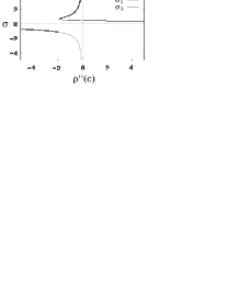
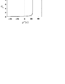
Figure 1: Variation of optimal $\sigma$ with $\rho^{\prime\prime}(c)$ for $C_{1}=C_{2}=1$, $d=1$, $\rho(c)=1$: (left) from pdf error minimisation and (right) from error of conditions minimisation.

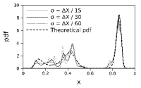
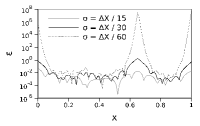
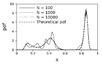
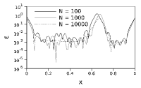
Figure 2: Pdf estimations and relative error of conditions obtained for: (first 2 graphics from left) $N=100$ and varying $\sigma$; (last 2 graphics) varying $N$ and $\sigma=\Delta X/30$.

References

[1] M. Abramowitz, I. A. Stegun (Eds.), Handbook of Mathematical Functions with Formulas, Graphs, and Mathematical Tables, 9th printing, Dover, New York, 1972, p. 17.
[2] E.T. Jaynes, Information Theory and Statistical Mechanics, Phys. Rev. 106 (1957) 620-630.
[3] S. Kirkpatrick, C.D. Gelatt Jr., M.P. Vecchi, Optimization by Simulated Annealing, Science 220 (1983) 671-680.
[4] E. Parzen, On Estimation of a Probability Density Function and Mode, Ann. Math. Statist. 33 (1962) 1065-1076.
[5] M.-I. Pop, Statistical distribution of some asteroid parameters, Bull. of the Transilvania University of Braşov III 4(53) (2011) 139-146.
[6] M.-I. Pop, Distribution of the daily sunspot number variation for the last 14 solar cycles, Solar Physics 276 (2012) 351-361.
[7] W.H. Press, S.A. Teukolsky, W.T. Vetterling, B.P. Flannery, Numerical Recipes: The Art of Scientific Computing, Third Edition, Cambridge University Press, 2007, pp. 228-229.
[8] M. Rosenblatt, Remarks on some nonparametric estimates of a density function, Ann. Math. Statist. 27 (1956) 832-837.