Estimations of the distances of stellar collapses in the galaxy by analyzing the energy spectrum of neutrino bursts
Abstract
The neutrino telescopes of the present generation, depending on their specific features, can reconstruct the neutrino spectra from a galactic burst. Since the optical counterpart could be not available, it is desirable to have at hand alternative methods to estimate the distance of the supernova explosion using only the neutrino data. In this work we present preliminary results on the method we are proposing to estimate the distance from a galactic supernova based only on the spectral shape of the neutrino burst and assumptions on the gravitational binding energy released an a typical supernova explosion due to stellar collapses.
1 Introduction
There is a consensus both in theoretical and experimental frameworks, the latter coming from observations of the SN1987A[2, 3, 4, 5], that a supernova explosion is preceeded by a huge neutrino flux of all flavours and their antiparticles. In principle, large neutrino telescopes are able to disentangle the neutrino burst signal from the background fluctuations, and to sample data with statistical significance to build the neutrino energy spectrum. The method proposed in this work is dedicated to estimate the distance from the collapsing star, i.e. the supernova explosion, by using only the information of the spectral shape from expected events on neutrino telescopes, as well as assumptions on the total binding energy of the stellar core released in the collapsing process. In this preliminary phase our discussion is focused on the errors of the method related to the theoretical uncertainties concerning the energy released in the formation of the compact object from the collapsing star.
2 Motivation
The distance from a galactic SN explosion determined by other methods can present some difficulties, for instance, the optical counterpart from galactic neutrino bursts can be fainted, introducing large errors in traditional photometry, or even obscured by the disk matter, making measurements in the visible spectrum completely unfeasible. Triangulation with other neutrino telescopes could result in large angular errors. Parameter scanning in data analysis is a possibility. In this case, the result of this method can be used as an independent input, or even as a prior in other statiscal methods such as a bayesian approach.
3 The Method
The number of expected events in a neutrino telescope, , is given by the expression:
| (1) |
Where is the number of target particles, is the SN neutrino spectrum, is the cross-section of the neutrino interaction to be detected and is the detection efficiency. D is the SN distance we are trying to estimate from data analysis. Supernova neutrino spectra are generally calculated by numerical methods and were obtained by different groups. We adopt the most standard approach, a Fermi-Dirac spectrum with a temperature T and a non-thermal parameter (pseudo-degeneracy) [6]:
| (2) |
Where and the normalization imposed by the total energy emitted as neutrinos, is the Fermi integral of 3rd order.
An important issue of the method is that can be related to the binding energy released in stellar collapse, since 99% of is carried away by neutrinos. The binding energy is given by[7]: . Considering that is tightly bound to the Chandrasekhar mass (1.2-1.4) and is the neutron star radius (12 - 15 km), thus is within a rather narrow range and consequently is constrained between . From Eq.1 one can see that an observation of a given number of counts by an experiment result as information only the ratio , i.e the normalization of the total neutrino flux diluted by the square of the collapse distance. We can go further if only from the spectral shape the parameters (T,) could be determined. Since is constrained as described above, by assuming a standard value for within a conservative range, it is possible to obtain the propper normalization constant for Eq.2 rather accurately. Then, we can solve Eq.1 for the distance , as it is the last free parameter.
The method can be summarized as follows: 1. A neutrino telescope measures events and builds their energy spectrum. 2. The Kolmogorov-Smirnov test is applied over data to determine spectral parameters (T, ). KS-test was specially chosen since is a test for shapes and it does not depend on relative normalizations of the distributions, thus at this step, and D are not relevant. 3. Counts from step 1. and parameters from data analysis (step 2.) are then used as inputs on the Eq.1, which is solved for D, by assuming as a prior the conservative, but nonetheless restrictive assumption erg as discussed before. We expect that the narrow range in can have minimum impact over the distance estimation. Simulations were used to evaluate the method sensitivity, as described in the next section.
4 Simulations
We selected for simulation the following parameters: (i) neutrino spectrum[6]: T= 3.0 MeV, ; (ii) erg; (iii) = 10 kpc. As a first case study we have taken the LVD experiment [8], running at the Gran Sasso underground laboratory (Italy) with 1 kton of active scintillator mass, target protons. The energy threshold was taken as . For simplicity, we have made .
Simulation steps: 1)Statistical fluctuations: is calculated from Eq.1, and then a random number is draw from a Poissonian distribution with mean , obtaining a new number of events ; 2)Simulation of experimental spectrum: values of energy are then draw following the distribution given by the integrand of Eq.1 ; 3) Experimental uncertainties: Each energy value from step (2) was properly fluctuated accordingly the energy resolution of the experiment[9]; 4)Systematics induced by uncertainties: Events bellow energy threshold are discarded; 5)End of the data set modelling: The resulting set of values are used as simulated experimental events to work as the neutrino energy spectrum.
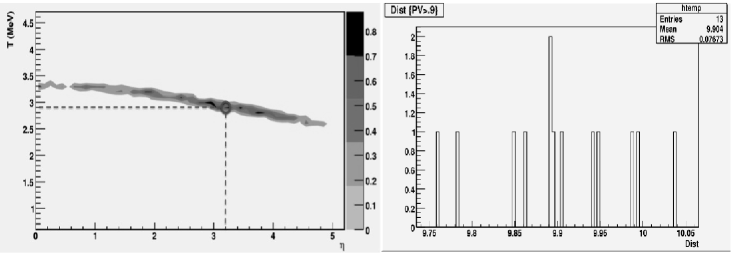
Analysis: In the proposed method, the KS-test is applied in a non-orthodox way: we scan a reasonable range for T and in very small steps, assuming each scanned pair (T, ) as a null hypothesis for the neutrino emission, . The (T, ) with greater KS probability pointed from the scan is chosen as the “best parametrization” (T,)∗. The corresponding values , (T,)∗, and the assumption for the analysis erg, are then used to solve Eq.1, as described before to obtain D. The Fig.1 shows in plane (T, ) the results for KS probability, obtained from the simulated spectra. Regardless the uncertainties that were introduced, only a small region of the parameter space has significant probability to be recognized as neutrino emission parameters. Moreover, the region’s boundary suggests a parameter correlation, explained by the mutually inverse action of parameters T and in the shape of the neutrino spectrum. In our study the best parametrization was found at (T,)∗ = (2.9, 3.1). The distribution of distances we found solving Eq.1 by selecting only the spectral parameters with KS-probability is also shown in figure 1. Despite the fluctuations that were introduced we have accurately determined the distance kpc. We also tested the opposite limit, simulating the SN explosion with erg but still assuming erg in the simulated data analysis, resulting in kpc.
5 Conclusions
The method to estimate the SN distance by neutrino spectral shape is very promising and was tested through simulations. When , we have obtained errors , meanwhile by testing over extreme limits, i.e. simulating the SN explosion with the lowest plausible energy and still assuming in the simulated data analysis the maximum plausible value for (see text for details) we have obtained errors . Enhancements on the simulations should be done by including different parameterization of neutrino spectra and more details on experimental uncertainties. Studies on the statistical distribution of should also be considered to obtain a more robust evaluation of the sensitivity of the method.
References
- [1] H.-Th. Janka et al., Phys. Rept. 442 (2007) 38
- [2] Aglietta, M. et al., Europhys. Lett., 3 (1987) 1315.
- [3] Hirata, K., et al., Phys. Rev. Lett., 58 (1987) 1490.
- [4] Bionta, R. M., et al., Phys. Rev. Lett., 58 (1987) 1494.
- [5] Alexeyev, E. N., et al., Pis’ma Zh. Eksp. Teor. Fiz., 45 (1987) 461; [JETPLett., 45 (1987) 589].
- [6] E.S.Myra and A.Burrows, Astrophys.J. 364 (1990) 222.
- [7] S. Shapiro, in Gravitational Radiation, ed. L. Smarr (Oxford University Press, E.U.A., 1978)
- [8] M.Aglieta et al., Il Nuovo Cimento A105 (1992) 1793.
- [9] P.Antonioli et al., Nucl. Instr. and Meth. 309A (1991) 569.