Gaia Universe Model Snapshot

Abstract

Context. This study has been developed in the framework of the computational simulations executed for the preparation of the ESA Gaia astrometric mission.

Aims. We focus on describing the objects and characteristics that Gaia will potentially observe without taking into consideration instrumental effects (detection efficiency, observing errors).

Methods. The theoretical Universe Model prepared for the Gaia simulation has been statistically analyzed at a given time. Ingredients of the model are described, giving most attention to the stellar content, the double and multiple stars, and variability.

Results. In this simulation the errors have not been included yet. Hence we estimate the number of objects and their theoretical photometric, astrometric and spectroscopic characteristics in the case that they are perfectly detected. We show that Gaia will be able to potentially observe 1.1 billion of stars (single or part of multiple star systems) of which about 2% are variable stars, 3% have one or two exoplanets. At the extragalactic level, observations will be potentially composed by several millions of galaxies, half million to 1 million of quasars and about 50,000 supernovas that will occur during the 5 years of mission. The simulated catalogue will be made publicly available by the DPAC on the Gaia portal of the ESA web site http://www.rssd.esa.int/gaia/

1 Introduction

The ESA Gaia astrometric mission has been designed for solving one of the most difficult yet deeply fundamental challenges in modern astronomy: to create an extraordinarily precise 3D map of about a billion stars throughout our Galaxy and beyond (Perryman et al. 2001).

The survey aims to reach completeness at $V_{\text{lim}}\sim 20-25$ mag depending on the color of the object, with astrometric accuracies of about 10$\mu$as at V=15. In the process, it will map stellar motions and provide detailed physical properties of each star observed: characterizing their luminosity, temperature, gravity and elemental composition. Additionally, it will perform the detection and orbital classification of tens of thousands of extra-solar planetary systems, and a comprehensive survey of some $10^{5}-10^{6}$ minor bodies in our solar system, as well as galaxies in the nearby Universe and distant quasars.

This massive stellar census will provide the basic observational data to tackle important questions related to the origin, structure and evolutionary history of our Galaxy and new tests of general relativity and cosmology.

It is clear that the Gaia data analysis will be an enormous task in terms of expertise, effort and dedicated computing power. In that sense, the Data Processing and Analysis Consortium (DPAC) is a large pan-European team of expert scientists and software developers which are officially responsible for Gaia data processing and analysis. The consortium is divided into specialized units with a unique set of processing tasks known as Coordination Units (CUs). More precisely, the CU2 is the task force in charge of the simulation needs for the work of other CUs, ensuring that reliable data simulations are available for the various stages of the data processing and analysis development. One key piece of the simulation software developed by CU2 for Gaia is the Universe Model that generates the astronomical sources.

The main goal of the present paper is to analyze the content of a full sky snapshot (for a given moment in time) of the Universe Model. With that objective in mind, the article has been organized in two main parts: in section 2, the principal components of the Gaia simulator are exposed, while the results of the analysis are detailed in section 3, complemented with a wide variety of diagrams and charts for better understanding.

In order to understand those results, it is important to remark that four passbands (and their corresponding magnitudes) are associated with the Gaia instruments: $G$, $G_{\mathrm{BP}}$ , $G_{\mathrm{RP}}$ and $G_{\mathrm{\mathrm{missing}}}{RVS}$ (see fig. 1.1).

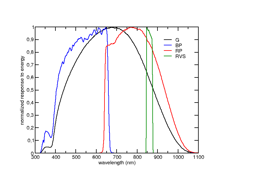
Figure 1.1: Gaia $G$, $G_{\mathrm{BP}}$ , $G_{\mathrm{RP}}$ and $G_{\mathrm{RVS}}$ passbands

As described in Jordi et al. (2010), from the astrometric measurements of unfiltered (white) light, Gaia will yield $G$ magnitudes in a very broad band covering the $350\text{\textendash}1000$ nm wavelength range. The $G$ band can be related to Johnson-Cousins V and I_C passband by the following approximation (Jordi et al. 2010) for unreddened stars :

$$G=V-0.0257-0.0924\;(V-I_{C})-0.1623\;(V-I_{C})^{2}+\\ +0.0090\;(V-I_{C})^{3}$$ (1.1)

for $-0.4<V-I\lesssim 6$ . The approximation can be simplifed to $G-V=0.0\pm 0.1$ for the range $-0.4<V-I<1.4$.

Besides, the spectrophotometric instrument (Jordi et al. 2010) consists on two low-resolution slitless spectrographs named ’Blue Photometer’ (BP) and ’Red Photometer’ (RP). They cover the wavelength intervals $330\text{\textendash}680$ nm and $650\text{\textendash}1050$ nm, and its total flux will yield $G_{\mathrm{BP}}$ and $G_{\mathrm{RP}}$ magnitudes. Additionally, for the brighter stars, Gaia also features a high-resolution ($R=11500$) integral field spectrograph in the range $847\text{\textendash}874$ nm around CaII triplet named Radial Velocity Spectrometer or RVS instrument. Its integrated flux will provide the $G_{\mathrm{RVS}}$ magnitude.

The RVS will provide the radial velocities of stars up to $G_{\mathrm{RVS}}=17$ with precisions ranging from 15 km s^-1 at the faint end to 1 km s^-1 or better at the bright end. Individual abundances of key chemical elements (e.g. Ca, Mg and Si) will be derived for stars up to $G_{\mathrm{RVS}}=12$.

Colour equations to transform Gaia photometric systems to the Johnson, SDSS and Hipparcos photometric systems can be found in Jordi et al. (2010).

The catalogue described in this paper will be made publicly available by the DPAC on the Gaia portal of the ESA web site http://www.rssd.esa.int/gaia/

2 Gaia simulator

Gaia will acquire an enormous quantity of complex and extremely precise data that will be transmitted daily to a ground station. By the end of Gaia’s operational life, around 150 terabytes ($10^{14}$ bytes) will have been transmitted to Earth: some 1000 times the raw volume from the related Hipparcos mission.

An extensive and sophisticated Gaia data processing mechanism is required to yield meaningful results from the collected data. In this sense, an automatic system has been designed to generate the simulated data required for the development and testing of the massive data reduction software.

The Gaia simulator has been organized around a common tool box (named GaiaSimu library) containing a universe model, an instrument model and other utilities, such as numerical methods and astronomical tools. This common tool box is used by several specialized components:

• Provides simulations of number counts and lists of observable objects from the universe model. It is designed to directly simulate catalog data.

• Simulates how the Gaia instruments will observe the sky at the pixel level, using realistic models of the astronomical sources and of the instrument properties.

• In charge of massive simulations of the raw telemetry stream generated by Gaia.

As a component of the GaiaSimu library, the universe model aims at simulating the characteristics of all the different types of objects that Gaia will observe: their spatial distribution, photometry, kinematics and spectra.

To handle the simulation, the sky is partitioned by a Hierarchical Triangular Mesh (HTM) (Kunszt et al. 2001), which subdivides the spherical surface into triangles in a recursive/multi level process which can be higher or lower depending on the area density. The first level divides the northern and southern sphere in four areas each, being identified by the letter N or S respectively and a number from 0 to 3. The second level for one of these areas (for instance, ’S1’) is generated by subdividing it in four new triangles as stated in figure 2.1. At each level, the area of the different triangles is almost the same.

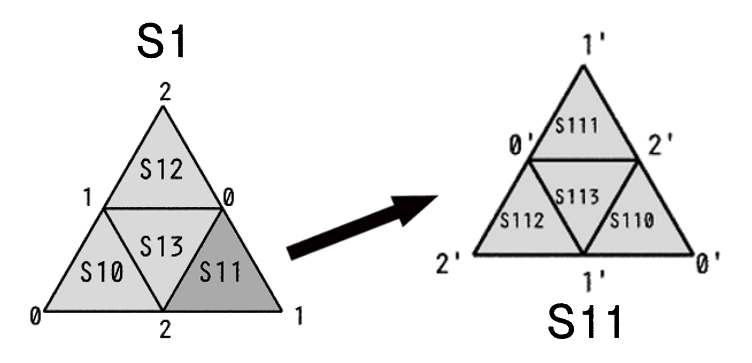
Figure 2.1: Hierarchical Triangular Mesh subdivisions scheme: Each triangle has three vertices labeled 0, 1 and 2. When the area is subdivided in 4 new triangles, the opposite midpoints are labeled 0’, 1’ and 2’, respectively, and the central triangle is suffixed with a 3.

The universe model is designed to generate lists of astronomical sources in given regions of the sky, represented by a concrete HTM area of a given maximum level. In the present simulation the HTM level is 8, giving a mean size of about 0.1 square degree for each triangular tile.

The distributions of these objects and the statistics of observables should be as realistic as possible, while the algorithms have been optimized in order that the simulations can be performed in reasonable time. Random seeds are fixed to regenerate the same sources at each new generation and in each of the 3 simulators.

The object generation process is divided into three main modules:

• Solar system object generator such as planets, satellites, asteroids, comets, etc. This generator is based on a database of known objects and has not been activated in the present statistical analysisTanga (2011).

• Galactic object generator based on the Besançon Galaxy model (BGM from now on). It creates stellar sources taking into account extinction, star variability, existence of binary systems and exoplanets.

• Extragalactic objects generator such as unresolved galaxies, QSO and supernovas.

In the following subsections, the generation of the different types of objects and the computation of their relevant characteristics are described.

2.1 Galactic objects

Galactic objects are generated from a model based on BGM (Robin et al. 2003) which provides the distribution of the stars, their intrinsic parameters and their motions. The stellar population synthesis combines:

• Theoretical considerations such as stellar evolution, galactic evolution and dynamics.

• Observational facts such as the local luminosity function, the age-velocity dispersion relation, the age-metallicity relation.

The result is a comprehensive description of the stellar components of the Galaxy with their physical characteristics (e.g. temperature, mass, gravity, chemical composition and motions).

The Galaxy model is formed by four stellar populations constructed with different model parameters. For each population the stellar content is defined by the Hess diagram according to the age and metallicity characteristics. The populations considered here are:

• The thin disc: young stars with solar metallicity in the mean. It is additionally divided in seven isothermal components of ages varying from 0–0.15 Gyr for the youngest to 7–10 Gyr for the oldest.

• The thick disc: in terms of metallicity, age and kinematics, stars are intermediate between the thin disc and the stellar halo.

• The stellar halo (spheroid): old and metal poor stars.

• The outer bulge: old stars with metallicities similar to the ones in the thin disc.

The simulations are done using the equation of stellar statistics. Specifying a direction and a distance $r_{\text{max}}$, the model generates a star catalog using the following equation:

$$N=\int_{0}^{r_{\text{max}}}\sum_{i=1}^{n}\rho_{i}\left(R,\theta,z,Age\right)\times\Phi\left(M_{V},T_{\mathrm{eff}},Age\right)\omega r^{2}dr$$ (2.1)

where $\rho\left(R,\theta,z,Age\right)$ is the stellar density law with galactocentric coordinates $\left(R,\theta,z\right)$, also described in table 2.1, $\Phi\left(M_{V},T_{\mathrm{eff}},Age\right)$ is the number of stars per square parsec in a given cell of the HR Diagram ($M_{V},T_{\mathrm{eff}},$Age) for a given age range near the sun, $\omega$ is the solid angle and $r$ the distance to the sun.

The functions $\rho\left(R,\theta,z,Age\right)$ (density laws) and $\Phi\left(M_{V},T_{\mathrm{eff}},Age\right)$ (Hess diagrams) are specific for each population, and established using theoretical and empirical constraints, as described below.

In a given volume element having an expected density of N, $\approx$ N stars are generated using a Poisson distribution. After generating the corresponding number of stars, each star is assigned its intrinsic attributes (age, effective temperature, bolometric magnitude, $U,V,W$ velocities, distance) and corresponding observational parameters (apparent magnitudes, colors, proper motions, radial velocities, etc) and finally affected by the implemented 3D extinction model from Drimmel et al. (2003).

2.1.1 Density laws

Table 2.1: Local mass density $\rho_{0}$ for different populations. Axis ratio $\epsilon$ are given as a function of age for the disc population and the spheroid.

Population	Age (Gyr)	Local density $\left(M_{\odot}\mathrm{pc}^{-3}\right)$	$\epsilon$
Disc	0–0.15	$4.0\times 10^{-3}$	0.0140
	0.15–1	$7.9\times 10^{-3}$	0.0268
	1–2	$6.2\times 10^{-3}$	0.0375
	2–3	$4.0\times 10^{-3}$	0.0551
	3–5	$4.0\times 10^{-3}$	0.0696
	5–7	$4.9\times 10^{-3}$	0.0785
	7–10	$6.6\times 10^{-3}$	0.0791
	WD	$3.96\times 10^{-3}$	-
Thick disc	11	$1.34\times 10^{-3}$	-
	WD	$3.04\times 10^{-4}$	-
Spheroid	14	$9.32\times 10^{-6}$	0.76

Density laws allow to extrapolate what is observed in the solar neighbourhood (i.e. local densities) to the rest of the Galaxy. The density law of each population has been described in Robin et al. (2003). However the disc and bulge density have been slightly changed. Revised density laws are given in table 2.3. It is worth noting that the local density assigned to the seven sub-populations of the thin disc and its scale height $z$ has been defined by a dynamically self-consistent process using the Galactic potential and Boltzman equations (Bienayme et al. 1987). In this table for simplicity the density formulae do not include the warp and flare, which are added as a modification of the position and thickness of the mid-plane.

The flare is the increase of the thickness of the disc with galactocentric distance:

$$k_{\mathrm{flare}}=1.+g_{\mathrm{flare}}\times\left(R-R_{\mathrm{flare}}\right)$$ (2.2)

with $g_{\mathrm{flare}}=0.545\times 10^{-6}\leavevmode\nobreak\ \mathrm{pc}^{-1}$ and $R_{\mathrm{flare}}=9500$ pc. The warp is modeled as a symmetrical S-shape warp with a linear slope of 0.09 starting at galactocentric distance of 8400 pc (Reylé et al. 2009). Moreover a spiral structure has been added with 2 arms, as determined in a preliminary study by De Amores & Robin (in prep.). The parameters of the arms are given in table 2.2.

Table 2.2: Parameters of the 2 arms of the spiral structure.

Parameter	1st arm	2nd arm
Internal radius in kpc	3.426	3.426
Pitch angle in radian	4.027	3.426
Phase angle of start in radian	0.188	2.677
Amplitude	1.823	2.013
Thickness in the plane	4.804	4.964

Table 2.3: Density laws where $\rho_{0}$ is the local mass density, $d_{0}$ a normalization factor to have a density of 1 at the solar position, $k_{\mathrm{flare}}$ the flare factor and $a=\sqrt{R^{2}+\left(\frac{z}{\epsilon}\right)^{2}}$ in kpc with $\epsilon$ being the axis ratio and ($R,z$) the cylindrical galactic coordinates. Local density $\rho_{0}$ and axial ratio $\epsilon$ can be found in table 2.1. For simplicity the disc density law is given here without the warp and flare (see text for their characteristics). For the bulge, $x,y,z$ are in the bulge reference frame and values of $N,\,x_{0},\,y_{0},\,z_{0},\,R_{c}$ as well as angles from the main axis to the Galaxy reference frame are given in Robin et al. (2003), table 5.

Population	Density laws
Disc	$\rho_{0}/d_{0}/k_{\mathrm{flare}}\times\left\{e^{-\left(\frac{a}{h_{R_{+}}}\right)^{2}}-e^{-\left(\frac{a}{h_{R_{-}}}\right)^{2}}\right\}$ with $h_{R_{+}}=5000$ pc and $h_{R_{-}}=3000$ pc	if age $\leq 0.15$ Gyr
	$\rho_{0}/d_{0}/k_{\mathrm{flare}}\times\left\{e^{-\left(0.25+\frac{a^{2}}{h_{R_{+}}^{2}}\right)^{\frac{1}{2}}}-e^{-\left(0.25+\frac{a^{2}}{h_{R_{-}}^{2}}\right)^{\frac{1}{2}}}\right\}$ with $h_{R_{+}}=2530$ pc and $h_{R_{-}}=1320$ pc	if age $>0.15$ Gyr
Thick disc	$\rho_{0}/d_{0}/k_{\mathrm{flare}}\times e^{-\frac{R-R_{\odot}}{h_{R}}}\times\left(1-\frac{1/h_{z}}{x_{l}\times\left(2.+x_{l}/h_{z}\right)}\times z^{2}\right)$	if $\left|z\right|\leq x_{l},x_{l}=72$ pc
	$\rho_{0}\times e^{-\frac{R-R_{\odot}}{h_{R}}}\times\frac{e^{x_{l}/h_{z}}}{1+x_{l}/2h_{z}}e^{-\frac{\left|z\right|}{h_{z}}}$ with $h_{R}=4000$ pc and $h_{z}=1200$ pc	if $\left|z\right|>x_{l},x_{l}=72$ pc
Spheroid	$\rho_{0}/d_{0}\times\left(\frac{a_{c}}{R_{\odot}}\right)^{-2.44}$	if $a\leq a_{c},\,a_{c}=500$ pc
	$\rho_{0}\times\left(\frac{a}{R_{\odot}}\right)^{-2.44}$	if $a>a_{c},\,a_{c}=500$ pc
Bulge	$N\times e^{-0.5\times r_{s}^{2}}$	$\sqrt{x^{2}+y^{2}}<R_{c}$
	$N\times e^{-0.5\times r_{s}^{2}}\times e^{-0.5\left(\frac{\sqrt{x^{2}+y^{2}}}{0.5}\right)^{2}}$ with $r_{s}^{2}=\sqrt{\left[\left(\frac{x}{x_{0}}\right)^{2}+\left(\frac{y}{y_{0}}\right)^{2}\right]^{2}+\left(\frac{z}{z_{0}}\right)^{4}}$	$\sqrt{x^{2}+y^{2}}>R_{c}$

2.1.2 Magnitude - Temperature - Age distribution

The distribution of stars in the HR diagram $\Phi\left(M_{V},T_{\mathrm{eff}}\right)$ is based on the Initial Mass Function (IMF) and Star Formation Rate (SFR) observed in the solar neighbourhood (see table 2.4). For each population, the SFR determines how much stellar mass is created at a given formation epoch, while the IMF distributes this mass into stars of different sizes. Then, the model brings every star created in each formation epoch to the present day considering evolutionary tracks and the population age.

For the thin disc, the distribution in the Hess diagram splits into several age bins. It is obtained from an evolutionary model which starts with a mass of gas, generates stars of different masses assuming an IMF and a SFR history, and makes these stars evolve along evolutionary tracks. The evolution model is described in Haywood et al. (1997a, b). It produces a file describing the distribution of stars per element volume in the space ($M_{V}$, T_eff, Age). Similar Hess diagrams are also produced for the bulge, the thick disc and the spheroid populations, assuming a single burst of star formation and ages of 10 Gyr, 11 Gyr and 14 Gyr respectively using Bergbush & VandenBerg (1992) isochrones.

The stellar luminosity function is the one of primary stars (single stars, or primary stars in multiple systems) and is normalized to the luminosity functions in the solar neighbourhood (Reid et al. 2002).

A summary of age and metallicities, star formation history and IMF for each population is given in tables 2.4 and 2.5.

White dwarfs are taken into account using the Wood (1992) luminosity function for the disc and Chabrier (1999) for the halo. Bulge white dwarfs are not considered. Additionally, some rare objects such as Be stars, peculiar metallicity stars and Wolf Rayet stars have also been added (see section 2.1.6).

Table 2.4: IMF and SFR for each population for primary stars.

	Age (Gyr)	IMF	SRF
Disc	0-10	$\begin{aligned} f\left(m\right)=\frac{dn}{dm}\propto m^{-\alpha}\\ \alpha=1.1,0.07<m<0.6M_{\odot}\\ \alpha=1.6,0.6<m<1M_{\odot}\\ \alpha=3.0,m>1M_{\odot}\end{aligned}$	constant
Thick disc	11	$f\left(m\right)=\frac{dn}{dm}\propto m^{-0.5}$	one burst
Stellar halo	14	$f\left(m\right)=\frac{dn}{dm}\propto m^{-0.5}$	one burst
Bulge	10	$f\left(m\right)=\frac{dn}{dm}\propto m^{-2.35}$ for $m>0.7M_{\odot}$	one burst

2.1.3 Metallicity

Contrarily to Robin et al. (2003) metallicities [Fe/H] are computed through an empirical age-metallicity relation $\psi\left(Z,\mathrm{Age}\right)$ from Haywood (2008). The mean thick disc and spheroid metallicities have also been revised. For each age and population component the metallicity is drawn from a gaussian, with a mean and a dispersion as given in table 2.5. One also accounts for radial metallicity gradient for the thin disc, $-0.7$ dex/kpc, but no vertical metallicity gradient.

Table 2.5: Age, metallicity and radial metallicity gradients.

	Age (Gyr)	¡[Fe/H]¿ (dex)	$\frac{d\left[Fe/H\right]}{dR}$ (dex/kpc)
Disc	0–0.15 0.15–1 1–2 2–3 3–5 5–7 7–10	$0.01\pm 0.010$ $0.00\pm 0.11$ $-0.02\pm 0.12$ $-0.03\pm 0.125$ $-0.05\pm 0.135$ $-0.09\pm 0.16$ $-0.12\pm 0.18$	$-0.07$
Thick disc	11	$-0.50\pm 0.30$	$0.00$
Stellar Halo	14	$-1.5\pm 0.50$	$0.00$
Bulge	10	$0.00\pm 0.20$	$0.00$

2.1.4 Alpha elements - Metallicity relation

Alpha element abundances are computed as a function of the population and the metallicity. For the halo, the abundance in alpha element is drawn from a random around a mean value, while for the thin disc, thick disc, and bulge populations it depends on [Fe/H]. Formulas are given in table 2.6.

Table 2.6: Alpha element abundances and metallicity relation estimated from Bensby & Feltzing (2009) for the thin and thick disc, and Gonzales et al (2011) for the bulge.

	¡[$\alpha$/Fe]¿ (dex)	Dispersion
Disc	$0.01043-0.13\times\left[Fe/H\right]+0.197*[Fe/H]^{2}+0.1882*[Fe/H]^{3}$	$0.02$
Thick disc	$0.392-e^{1.19375\times\left[Fe/H\right]-1.3038}$	$0.05$
Stellar Halo	$0.4$	$0.05$
Bulge	$-0.334\times\left[Fe/H\right]+0.134$	$0.05$

2.1.5 Age - velocity dispersion

Age-velocity dispersion relation is obtained from Gomez et al. (1997) for the thin disc, while Ojha et al. (1996, 1999) determined the velocity ellipsoid of the thick disc, which has been used in the model (see table 2.7).

Table 2.7: Velocity dispersions, asymmetric drift $V_{ad}$ at the solar position and velocity dispersion gradient. W axis is pointing the north galactic pole, U the galactic center and V is tangential to the rotational motion. It is worth noting that $\frac{d\ln\left(\sigma_{U}^{2}\right)}{dR}=0.2$ for the disc.

	Age (Gyr)	$\sigma_{U}$ $\left(km\,s^{-1}\right)$	$\sigma_{V}$ $\left(km\,s^{-1}\right)$	$\sigma_{W}$ $\left(km\,s^{-1}\right)$	$V_{ad}$ $\left(km\,s^{-1}\right)$
Disc	0–0.15	16.7	10.8	6	3.5
	0.15–1	19.8	12.8	8	3.1
	1–2	27.2	17.6	10	5.8
	2–3	30.2	19.5	13.2	7.3
	3–5	36.7	23.7	15.8	10.8
	5–7	43.1	27.8	17.4	14.8
	7–10	43.1	27.8	17.5	14.8
Thick disc	11	67	51	42	53
Spheroid	14	131	106	85	226
Bulge	10	113	115	100	79

2.1.6 Stellar rotation

The rotation of each star is simulated following specifications from Cox et al. (2000). The rotation velocity is computed as a function of luminosity and spectral type. Then $vsini$ is computed for random values of the inclination of the star’s rotation axis.

2.1.7 Rare objects

For the needs of the simulator, some rare objects have been added to the BGM Hess diagram:

Be stars: this is a transient state of B-type stars with a gaseous disc that is formed of material ejected from the star (Be stars are typically variable). Prominent emission lines of hydrogen are found in its spectrum because of re-processing stellar ultraviolet light in the gaseous disc. Additionally, infrared excess and polarization is detected as a result from the scattering of stellar light in the disc.

Oe and Be stars are simulated as a proportion of 29% of O7-B4 stars, 20% of B5-B7 stars and 3% of B8-B9 stars (Jaschek et al. 1988; Zorec & Briot 1997). For these objects, the ratio between the envelope radius and the stellar radius is linked with the line strength in order to be able to determine their spectrum. Over the time, this ratio changes between 1.2 and 6.9 to simulate the variation of the emission lines.

Two types of peculiar metallicity stars are simulated, following Kurtz (1982); Kochukhov (2007); Stift & Alecian (2009), for A and B stars that have a much slower rotation than normal:

• Am stars have strong and often variable absorption lines of metals such as zinc, strontium, zirconium, and barium, and deficiencies of others, such as calcium and scandium. These anomalies with respect to A-type stars are due to the fact that the elements that absorb more light are pushed towards the surface, while others sink under the force of gravity.
  
  In the model, 12% of A stars on the main sequence in the $T_{\mathrm{eff}}$ range 7400 K - 10200 K are set to be Am stars. 70% of these Am stars belong to a binary system with period from 2.5 to 100 days. They are forced to be slow rotators: 67% have a projection of rotation velocity $v_{\mathrm{sin\,i}}<50$ km/s and 23% have $50<v_{\mathrm{sin\,i}}<100$ km/s.
  

• Ap/Bp stars present overabundances of some metals, such as strontium, chromium, europium, praseodymium and neodymium, which might be connected to the present stronger magnetic fields than classical A or B type star.
  
  In the simulation, 8% of A and B stars on the main sequence in the $T_{\mathrm{eff}}$ range 8000 K – 15000 K are set to be Ap or Bp stars. They are forced to have a smaller rotation : $v_{\mathrm{sin\,i}}<120$ km/s.
  

Wolf Rayet (WR) stars are hot and massive stars with a high rate of mass loss by means of a very strong stellar wind. There are 3 classes based on their spectra: the WN stars (nitrogen dominant, some carbon), WC stars (carbon dominant, no nitrogen) and the rare WO stars with C/O ¡ 1.

WR densities are computed following the observed statistics from the VIIth catalogue of Galactic Wolf-Rayet stars of van der Hucht (2001). The local column density of WR stars is $2.9\times 10^{\text{\textminus}6}\mathrm{pc}^{\text{\textminus}2}$ or volume density $2.37\times 10^{\text{\textminus}8}\mathrm{pc}^{\text{\textminus}3}$. Among them, 50% are WN, 46% are WC and 3.6% are WO. The absolute magnitude, colors, effective temperature, gravity and mass have been estimated from the literature. The masses and effective temperature vary considerably from one author to another. As a conservative value, it is assumed that the WR stars have masses of 10 $M_{\odot}$ in the mean, an absolute V magnitude of -4, a gravity of -0.5, and an effective temperature of 50,000 K.

2.1.8 Binary systems

The BGM model produces only single stars which densities have been normalized to follow the luminosity function (LF) of single stars and primaries in the solar neighbourhood (Reid et al. 2002). The IMF, inferred from the LF and the mass-luminosity relation, goes down to the hydrogen burning limit, and include disc stars down to $M_{V}=24$. It corresponds to spectral types down to about L5.

In the Gaia simulation multiple star systems are generated with some probability (Arenou 2011) increasing with the mass of the primary star obtained from the BGM model.

The mass of the companion is then obtained through a given statistical relation $q=\frac{M_{2}}{M_{1}}=f\left(M_{1}\right)$ which depends on period and mass ranges, ensuring that the total number of stars and their distribution is compatible with the statistical observations and checking that the pairing is realistic. The mass and age of secondary determine physical parameters computed using the Hess diagram distribution in the Besançon model. Although, for the case of PMS stars, it appears that pairing has been done is some cases with main sequence stars due to the resolution in age which is not good enough to distinguish them. It will be improved in further simulations.

It is worth noting that while, observationally, the primary of a system is conventionally the brighter, the model uses here the other convention, i.e. the primary is the one with the largest mass, and consequently the generated mass ratio is constrained to be $0<q\leq 1$.

The separation of the components (AU) is chosen with a Gaussian probability with different mean values depending on the stars’ masses (a smaller average separation for low mass stars). Through Kepler’s third law, the separation and masses then give the orbital period. The average orbital eccentricity (a perfect circular orbit corresponds to $e=0$) depends on the period by the following relation:

$$E\left[e\right]=a\left(b-e^{-c\log\left(P\right)}\right)$$ (2.3)

where $a,b,c$ are constant with different values depending on the star’s spectral type (values can be found in table 1 of Arenou (2010))

To describe the orientation of the orbit, three angles are chosen randomly:

• The argument of the periastron $\omega_{2}$ uniformly in $\left[0,\,2\pi\right[$,

• The position angle of the node $\Omega$ uniformly in $\left[0,\,2\pi\right[$

• The inclination $i$ uniformly random in $\cos\left(i\right)$.

The moment at which stars are closest together (the periastron date $T$) is also chosen uniformly between 0 and the period $P$.

A large effort has been put at trying to ensure that simulated multiple stars numbers are in accordance with latest fractions known from available observations. A more detailed description can be found in Arenou (2011).

Although the present paper describes the content of the Universe Model at a fixed moment in time, it should be reminded that the model is being used to simulate the Gaia observations. Thus, obviously, the astrometric, photometric and spectroscopic observables of a multiple system vary in time according to the orbital properties. This means that e.g. the apparent path of the photocentre of an unresolved binary will reflect the orbital motion through positional and radial velocity changes, or that the light curve of an eclipsing binary will vary in each band.

2.1.9 Variable stars

• Regular and semi-regular variables

Depending on their position in the HR Diagram, the generated stars have a probability of being one of the six types of regular and semi-regular variable stars considered in the simulator:

Cepheids:

Supergiant stars which undergo pulsations with very regular periods on the order of days to months. Their luminosity is directly related to their period of variation.

$\delta$Scuti:

Similar to Cepheids but rather fainter, and with shorter periods.

RR Lyrae:

Much more common than Cepheids, but also much less luminous. Their period is shorter, typically less than one day. They are classified into

RRab:

Asymmetric light curves (they are the majority type).

RRc:

Nearly symmetric light curves (sometimes sinusoidal).

Gamma Doradus:

Display variations in luminosity due to non-radial pulsations of their surface. Periods of the order of one day.

RoAp:

Rapidly oscillating Ap stars are a subtype of the Ap star class (see section 2.1.7) that exhibits short-timescale rapid photometric or radial velocity variations. Periods on the order of minutes.

ZZceti:

Pulsating white dwarf with hydrogen atmosphere. These stars have periods between seconds to minutes.

Miras:

Cool red supergiants, which are undergoing very large pulsations (order of months).

Semiregular:

Usually red giants or supergiants that show a definite period on occasion, but also go through periods of irregular variation. Periods lie in the range from 20 to more than 2000 days.

ACV ($\alpha$ Canes Venaticorum):

Stars with strong magnetic fields whose variability is caused by axial rotation with respect to the observer.

A summary of the variable type characteristics is given in table 2.8 and the description of their light curve is given in table 2.9

Table 2.8: Characteristics of the variable types. Localization in the (spectral type, luminosity class) diagram, probability of a star to be variable in this region, stellar population and metallicity range which are concerned.

Type	Spec.	Lum.	Proba	Pop	[Fe/H]
$\delta$ Scuti (a)	A0:F2	III	0.3	all	all
$\delta$ Scuti (b)	A1:F3	IV:V	0.3	all	all
ACV (a)	B5:B9	V	0.016	thin disc	-1 to 1
ACV (b)	A0:A8	IV:V	0.01	thin disc	-1 to 1
Cepheid	F5:G0	I:III	0.3	thin disc	-1 to 1
RRab	A8:F5	III	0.4	spheroid	all
RRc	A8:F5	III	0.1	spheroid	all
RoAp	A0:A9	V	0.001	thin disc	-1 to 1
SemiReg (a)	K5:K9	III	0.5	all	all
SemiReg (b)	M0:M9	III	0.9	all	all
Miras	M0:M9	I:III	1.0	all	all
ZZCeti	White dwarf	-	1.0	all	all
GammaDor	F0:F5	V	0.3	all	all

Period and amplitude are taken randomly from a 2D distribution defined for each variability type (Eyer et al. 2005). For Cepheids, a period-luminosity relation is also included log(P)=$(-M_{V}+1.42)/2.78$ (Molinaro et al. 2011). For Miras the relation is log(P)=$(-M_{\mathrm{Bol}}+2.06)/2.54$ (Feast et al. 1989). The different light curve models for each variability type are described in Reylé et al. (2007).

The variation of the radius and radial velocity are computed accordingly to the light variation, for stars with radial pulsations (RRab, RRc, Cepheids, $\delta$ Scuti, SemiRegular, and Miras).

Table 2.9: Light curves of the regular or semi-regular variable stars where $\omega\,_{t}=2\pi\frac{t}{P}+\phi$ ($P$ is the period, $\phi$ is the phase)

Type	Light curve
Cepheid	$\begin{aligned} S=&0.148\sin\left(\omega\,_{t}-20.76\right)+0.1419\sin\left(2\omega\,_{t}-63.76\right)\\ &+0.0664\sin\left(3\omega\,_{t}-91.57\right)+0.0354\sin\left(4\omega\,_{t}-112.62\right)\\ &+0.020\sin\left(5\omega\,_{t}-129.47\right)\end{aligned}$
$\delta$ Scuti, RoAp, RRc, Miras	$S=0.5\sin\left(\omega\,_{t}\right)$
ACV	$S=-0.5\cos\left(2\omega\,_{t}\right)\frac{1-f\times\cos\left(\omega\,_{t}\right)}{1+f/2}$ where $f$ is a random number in [0;1]
SemiReg	Inverse Fourier Transform of a gaussian in frequency space

• Dwarf and classical novae

Dwarf novae and Classical novae are cataclysmic variable stars consisting of close binary star systems in which one of the components is a white dwarf that accretes matter from its companion.

Classical novae result from the fusion and detonation of accreted hydrogen, while current theory suggests that dwarf novae result from instability in the accretion disc that leads to releases of large amounts of gravitational potential energy. Luminosity of dwarf novae is lower than classical ones and it increases with the recurrence interval as well as the orbital period.

The model simulates half of the white dwarfs in close binary systems with period smaller than 14 hours as dwarf novae. The light curve is simulated by a linear increase followed by an exponential decrease. The time between two bursts, the amplitude, the rising time and the decay time are drawn from gaussian distributions derived from OGLE observations (Wyrzykowski & Skowron, private communication).

The other half of white dwarfs in such systems is simulated as a Classical novae.

• M-dwarf flares

Flares are due to magnetic reconnection in the stellar atmospheres. These events can produce dramatic increases in brightness when they take place in M dwarfs and brown dwarfs.

The statistics used in the model for M-dwarf flares are mainly based on Kowalski et al. (2009) and their study on SDSS data: 0.1% of M0-M1 dwarfs, 0.6% of M2-M3 dwarfs, and 5.6% of M4-M6 dwarfs are flaring. The light curve for magnitude $m$ is described as follows:

$$f =1+e^{-\left(t-t_{0}\right)/\tau} \,t>t_{0}$$

$$f =1 \,t<t_{0}$$ (2.4)

$$m =m_{0}-1.32877\times A\times 2.5\times\log\left(f\right)$$

where $t_{0}$ is the time of the maximum, $\tau$ is the decay time (in days, random between 1 and 15 minutes), $m_{0}$ is the baseline magnitude of the source star, $A$ is the amplitude in magnitudes (drawn from a gaussian gaussian distribution with $\sigma=1$ and $x_{0}=1.2$).

• Eclipsing binaries

Eclipsing binaries, while being variables, are treated as binaries and the eclipses are computed from the orbits of the components. See section 2.1.8.

• Microlensing events

Gravitational microlensing is an astronomical phenomenon due to the gravitational lens effect, where distribution of matter between a distant source and an observer is capable of bending (lensing) the light from the source. The magnification effect permits the observation of faint objects such as brown dwarfs.

In the model, microlensing effects are generated assuming a map of event rates as a function of Galactic coordinates $(l,b)$. The probabilities of lensing over the sky are drawn from the study of Han (2008). This probabilistic treatment is not based on the real existence of a modelled lens close to the line of sight of the source, it simply uses the lensing probability to randomly generate microlensing events for a given source during the five year observing period.

The Einstein crossing time is also a function of the direction of observation in the bulge, obtained from the same paper. The Einstein time of the simulated events are drawn from a gaussian distribution centered on the mean Einstein time. The impact parameter follows a flat distribution from 0 to 1. The time of maximum is uniformely distributed and completely random, from the beginning to the end of the mission. The Paczynski formula (Paczynski 1986) is used to compute the light curve.

2.1.10 Exoplanets

One or two extra-solar planets are generated with distributions in true mass $M_{p}$ and orbital period $P$ resembling those of Tabachnik & Tremaine (2002) which constitutes quite a reasonable approximation to the observed distributions as of today, and extrapolated down to the masses close to the mass of Earth. A detailed description can be found in Sozzetti et al. (2009).

Semi-major axes are derived given the star mass, planet mass, and period. Eccentricities are drawn from a power-law-type distribution, where full circular orbits ($e=0.0$) are assumed for periods below 6 days. All orbital angles ($i$, $\omega$ and $\Omega$) are drawn from uniform distributions. Observed correlations between different parameters (e.g, $P$ and $M_{p}$ ) are reproduced.

Simple prescriptions for the radius (assuming a mass-radius relationship from available structural models, see e.g. Baraffe et al. (2003)), effective temperature, phase, and albedo (assuming toy models for the atmospheres, such as a Lambert sphere) are provided, based on the present-day observational evidence.

For every dwarf star generated of spectral type between F and mid-K, the likelihood that it harbours a planet of given mass and period depends on its metal abundance according to the Fischer & Valenti (2005) and Sozzetti et al. (2009) prescriptions. M dwarfs, giant stars, white dwarfs, and young stars do not include simulated planets for the time being, as well as double and multiple systems.

The astrometric displacement, spectroscopic radial velocity amplitude, and photometric dimming (when transiting) induced by a planet on the parent star, and their evolution in time, are presently computed from orbital components similarly to double stellar systems.

2.2 Extragalactic objects

2.2.1 Resolved galaxies

In order to simulate the Magellanic clouds, catalogues of stars and their characteristics (magnitudes $B$, $V$, $I$, $T_{\mathrm{eff}}$, $log(g)$, spectral type) have been obtained from the literature (Belcheva et al., private communication).

For the astrometry, since star by star distance is missing, a single proper motion and radial velocity for all stars of both clouds is assumed. Chemical abundances are also guessed from the mean abundance taken from the literature. The resulting values and their references are given in table 2.10. For simulating the depth of the clouds a gaussian distribution is assumed along the line of sight with a sigma given in the table.

Table 2.10: Assumed parameters of the Magellanic clouds.

Parameter	Units	LMC	SMC	Reference
Distance	kpc	48.1	60.6	LMC: Macri et al. (2006)
				SMC: Hilditch et al. (2005)
Depth	kpc	0.75	1.48	LMC: Sakai et al. (2000)
				SMC: Subramanian (2009)
$\mu_{\alpha}\cos\left(\delta\right)$	mas/yr	1.95	0.95	Costa et al. (2009)
$\mu_{\delta}$	mas/yr	0.43	-1.14	Costa et al. (2009)
$V_{\text{los}}$	km/s	283	158	SIMBAD (CDS)
$[Fe/H$]	dex	-0.75$\pm$0.5	-1.2$\pm$0.2	Kontizas et al, (2011)
$[\alpha/Fe]$	dex	0.00$\pm$0.2	0.00$\pm$0.5	Kontizas et al, (2011)

Stellar masses are estimated for each star from polynomial fits of the mass as a function of $B-V$ colour, for several ranges of $\log(g)$, based on Padova isochrones for a metallicity of $z=0.003$ for the LMC and $z=0.0013$ for the SMC. The gravities have been estimated from the effective temperature and luminosity class but is very difficult to assert from the available observables. Hence the resulting HR diagrams for the Magellanic clouds are not as well defined and reliable as they would be from theoretical isochrones.

2.2.2 Unresolved galaxies

Most galaxies observable by Gaia will not be resolved in their individual stars. These unresolved galaxies are simulated using the Stuff (catalog generation) and Skymaker (shape/image simulation) codes from Bertin (2009), adapted to Gaia by Dollet (2004) and (Krone-Martins et al. 2008).

This simulator generates a catalog of galaxies with a 2D uniform distribution and a number density distribution in each Hubble type sampled from Schechter’s luminosity function (Fioc & Rocca-Volmerange 1999). Parameters of the luminosity function for each Hubble type are given in table 2.11. Each galaxy is assembled as a sum of a disc and a spheroid, they are located at their redshift and luminosity and K corrections are applied. The algorithm returns for each galaxy its position, magnitude, B/T relation, disc size, bulge size, bulge flatness, redshift, position angles, and $V-I$.

The adopted library of synthetic spectra at low resolution has been created Tsalmantza et al. (2009) based on Pegase-2 code (Fioc & Rocca-Volmerange 1997)(http://www2.iap.fr/pegase). 9 Hubble types are available (including Quenched Star Forming Galaxies or QSFG) Tsalmantza et al. (2009), with 5 different inclinations (0.00, 22.5, 45.0, 67.5, 90.0) for non-elliptical galaxies, and at 11 redshifts (from 0. to 2. by step of 0.2). For all inclinations, Pegase-2 spectra are computed with internal extinction by transfer model with two geometries either slab or spheroid depending on type.

It should be noted that the resulting percentages per type, given in Table 3.13, reflect the numbers expected without applying the Gaia source detection and prioritization algorithms. De facto, the detection efficiency will be better for unresolved galaxies having a prominent bulge and for nucleated galaxies, hence the effective Gaia catalog will have different percentages than the ones given in the table.

Table 2.11: Parameters defining the luminosity function for different galaxy types at $z=0$, from Fioc & Rocca-Volmerange (1999). The LF follows a shape from Schechter (1976). M* (Bj) is the magnitude in the Bj filter in the Schechter formalism.

Type	$\phi$* ($Mpc^{-3}$)	M* (Bj)	Alpha	Bulge/Total
E2	$1.91\times 10^{-3}$	$-20.02$	$-1$	$1.0$
E-SO	$1.91\times 10^{-3}$	$-20.02$	$-1$	$0.9$
Sa	$2.18\times 10^{-3}$	$-19.62$	$-1$	$0.57$
Sb	$2.18\times 10^{-3}$	$-19.62$	$-1$	$0.32$
Sbc	$2.18\times 10^{-3}$	$-19.62$	$-1$	$0.32$
Sc	$4.82\times 10^{-3}$	$-18.86$	$-1$	$0.016$
Sd	$9.65\times 10^{-3}$	$-18.86$	$-1$	$0.049$
Im	$9.65\times 10^{-3}$	$-18.86$	$-1$	$0.0$
QSFG	$1.03\times 10^{-2}$	$-16.99$	$-1.73$	$0.0$

2.2.3 Quasars

QSOs are simulated from the scheme proposed in Slezak & Mignard (2007). To summarize, lists of sources have been generated with similar statistical properties as the SDSS, but extrapolated to G = 20.5 (the SDSS sample being complete to i = 19.1) and taking into account the flatter slope expected at the faint-end of the QSO luminosity distribution. The space density per bin of magnitude and the luminosity function should be very close to the actual sky distribution. Since bright quasars are saturated in the SDSS, the catalogue is complemented by the Véron-Cetty & Véron (2006) catalogue of nearby QSOs.

The equatorial coordinates have been generated from a uniform drawing on the sphere in each of the sub-populations defined by its redshift. No screening has been applied in the vicinity of the Galactic plane since this will result directly from the application of the absorption and reddening model at a later stage. Distance indicators can be derived for each object from its redshift value by specifying a cosmological model. Each of these sources lying at cosmological distances, a nearly zero ($10^{-6}$mas) parallax has been assigned to all of them (equivalent to an Euclidean distance of about 1 Gpc ) in order to avoid possible overflow/underflow problems in the simulation.

In principle, distant sources are assumed to be co-moving with the general expansion of the distant Universe and have no transverse motion. However, the observer is not at rest with respect to the distant Universe and the accelerated motion around the Galactic center, or more generally, that of the Local group toward the Virgo cluster is the source of a spurious proper motion with a systematic pattern. This has been discussed in many places (Kovalevsky 2003; Mignard 2005). Eventually the effect of the acceleration (centripetal acceleration of the solar system) will show up as a small proper motion of the quasars, or stated differently we will see the motion of the quasars on a tiny fraction of the aberration ellipse whose period is 250 million years. This effect is simulated directly in the quasar catalogue, and equations given in Slezak & Mignard (2007). This explains their not null proper motions in the output catalogue.

2.2.4 Supernovae

A set of supernovae (SN) are generated associated with galaxies, with a proportion for each Hubble type, as given in table 2.12. Numbers of SNIIs are computed from the local star formation rate at 13Gyrs (z=0) and IMF for M*(Bj) galaxy types as predicted by the code PEGASE.2. Theoretical SNIa numbers follow the SNII/SNIa ratios from Greggio & Renzini (1983). In this case, the SN is situated at a distance randomly selected at less than a disc radius from the parent galaxy, accounting for the inclination.

Table 2.12: Predictions of SNII and SNIa numbers exploding per century for M* (Bj) galaxies defined in table 2.11.

Hubble type	SNII /century	SNI /century
E2	0.0	0.05
E-S0	0.0	0.05
Sa	0.4	0.11
Sb	0.62	0.13
Sbc	1.07	0.16
Sc	0.16	0.07
Sd	0.049	0.07
Im	0.60	0.05
QSFG	0.0	0.05

Another set of SN are generated randomly on the sky to simulate SN on host galaxies which are too faint in surface brightness to be detected by Gaia.

Four SN types are available with a total probability of occuring determined to give at the end 6366 SN per steradian during the 5 year mission (from estimations by Belokurov & Evans (2003)). For each SN generated a type is attributed from the associated probability, and the absolute magnitude is computed from a Gaussian drawing centered on the absolute magnitude and the dispersion of the type corresponding to the cosmic scatter. These parameters are given in table 2.13. Supernova light curves are from Peter Nugent. It is assumed that the SN varies the same way at each wavelength and the light curve in V has been taken as reference.

Table 2.13: Parameters for each supernova type taken from Belokurov & Evans (2003). The probability is given for each type, as well as the absolute magnitude and a dispersion about this magnitude corresponding to the cosmic variance.

Type	Probability	$M_{G}$	Sigma
Ia	0.6663	-18.99	0.76
Ib/Ic	0.0999	-17.75	1.29
II-L	0.1978	-17.63	0.88
II-P	0.0387	-16.44	1.23

2.3 Extinction model

The extinction model, applied to Galactic and extragalatic objects, is based on the dust distribution model of Drimmel et al. (2003). This full 3D extinction model is a strong improvement over previous generations of extinction models as it includes both a smooth diffuse absorption distribution for a disc and the spiral structure and smaller scale corrections based on the integrated dust emission measured from the far infrared (FIR). The extinction law is from Cardelli et al. (1989).

3 Gaia Universe Model Snapshot (GUMS)

The Gaia Universe Model Snapshot (GUMS) is part of the GOG component of the Gaia simulator. It has been used to generate a synthetic catalogue of objects from the universe model for a given static time $t_{0}$ simulating the real environment where Gaia will observe (down to $G=20$).

It is worth noting that this snapshot is what Gaia will be able to potentially observe but not what it will really detect, since satellite instrument specifications and the available error models are not taken into account in the present statistical analysis. Gaia performances and error models are described at http://www.rssd.esa.int/index.php?page=Science_Performance&project=GAIA.

The generated universe model snapshot has been analyzed by using the Gog Analysis Tool (GAT) statistics framework, which produces all types of diagnostic statistics allowing its scientific validation (e.g. star density distributions, HR diagrams, distributions of the properties of the stars). The visual representation of the most interesting results exposed in this article have been generated using Python, Healpy and Matplotlib (Hunter 2007).

The simulation was performed with MareNostrum, one of the most powerful supercomputers in Europe managed by the Barcelona Supercomputing Center. The execution took 20.000 hours (equivalent to 28 months) of computation time distributed in 20 jobs, each one using between 16 and 128 CPUs. MareNostrum runs a SUSE Linux Enterprise Server 10SP2 and its 2,560 nodes are powered by 2 dual-core IBM 64-bit PowerPC 970MP processors running at 2.3 GHz.

3.1 Galactic objects overview

• G less than 20 mag

In general terms, the universe model has generated a total number of 1,000,000,000 galactic objects of which ~49% are single stars and ~51% stellar systems formed by stars with planets and binary/multiple stars.

Individually, the model has created 1,600,000,000 stars where about 32% of them are single stars with magnitude G less than 20 (potentially observable by Gaia) and 68% correspond to stars in multiple systems (see table 3.1). This last group is formed by stars that have magnitude G less than 20 as a system but, in some cases, the isolated components can have magnitude G superior to 20 and won’t be individually detectable by Gaia.

Only taking into consideration the magnitude limit in G and ignoring the angular separation of multiple systems, Gaia could be able to individually observe up to 1,100,000,000 stars (69%) in single and multiple systems.

• $G_{\mathrm{RVS}}$ less than 17 mag

For $G_{\mathrm{RVS}}$ magnitudes limited to 17, the model has generated 370,000,000 galactic objects of which ~43% are single stars and ~57% stellar systems formed by stars with planets and binary/multiple stars.

Concretely, the RVS instrument could potentially provide radial velocities for up to 390,000,000 stars in single and multiple systems if the limit in angular separation and resolution power are ignored (see table 3.1).

• $G_{\mathrm{RVS}}$ less than 12 mag

The model has generated 13,100,000 galactic objects with $G_{\mathrm{RVS}}$ less than 12, of which ~27% are single stars and ~73% stellar systems formed by stars with planets and binary/multiple stars.

Again, if the limits in angular separation and resolution power are ignored, the RVS instrument could measure individual abundances of key chemical elements (metallicities) for ~13,000,000 stars (see table 3.1).

Table 3.1: Overview of the number of single stars and multiple system generated by the universe model. Percentages have been calculated over the total stars.

Stars	G ¡ 20 mag	Grvs ¡ 17 mag	Grvs ¡ 12 mag
Single stars	31.59%	25.82%	12.91%
Stars in multiple systems	68.41%	74.18%	87.09%
$\Rightarrow$ In binary systems	52.25%	51.55%	40.24%
$\Rightarrow$ Others (ternary, etc.)	16.16%	22.63%	46.85%
Total stars	1,600,000,000	600,000,000	28,000,000
Individually observable	1,100,000,000	390,000,000	13,000,000
$\Rightarrow$ Variable	1.78%	3.06%	8.37%
$\Rightarrow$ With planets	1.75%	1.44%	0.66%

3.2 Star distribution

The distribution of stars in the sky has been plotted using a Hierarchical Equal Area isoLatitude Pixelisation, also known as Healpix projection. Unlike the HTM internal representation of the sky explained in section 2, Healpix provide areas of identical size which are useful for comparison.

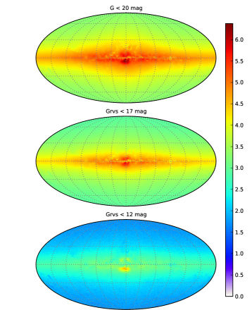
Figure 3.1: Total sky distribution of stars for different magnitudes. Top down: $G<20$, $G_{\mathrm{RVS}}<17$ and $G_{\mathrm{RVS}}<12$. Color scale indicates the $\log_{10}$ of the number of stars per square degree.

The number of stars on every region of the sky varies significantly depending on the band (figure 3.1) and the population (figure 3.2). In this last case, it is clear how the galactic center is concentrated in the middle of the galaxy with only 10% of stars, while the thin disc is the densest region (67%) as stated in table 3.2.

The effects of the extinction model due to the interstellar material of the Galaxy, predominantly atomic and molecular hydrogen and significant amounts of dust, is clearly visible in these representations of the sky.

Table 3.2: Stars by population. Percentages have been calculated over the total number of stars for each respective column.

Population	G ¡ 20 mag	Grvs ¡ 17 mag	Grvs ¡ 12 mag
disc	66.59%	76.82%	76.21%
Thick disc	21.88%	14.39%	8.75%
Spheroid	1.25%	0.58%	0.19%
Bulge	10.28%	8.22%	14.85%
Total	1,100,000,000	390,000,000	13,000,000

A projected representation in heliocentric-galactic coordinates of the stellar distribution shows how the majority of the generated stars are denser near the sun position, located at the origin of the XYZ coordinate system, and the bulge at 8.5 kpc away (figure 3.3). Specially from a top perspective (XY view), it is appreciable the extinction effect which produces windows where farther stars can be observed. One also notice the sudden density drop towards the anticenter which is due to the edge of the disc, assumed to be at a galactocentric distance of 14 kpc, following Robin et al. (1992).

The distribution of stars according to the G magnitude varies depending on the stellar population, being specially different for the bulge (figure 3.4).

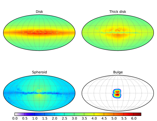
Figure 3.2: Stellar distribution split by population ($G<20$). Left to right, top down: thin disc, thick disc, spheroid and bulge. Color scale indicates the $\log_{10}$ of the number of stars per square degree.

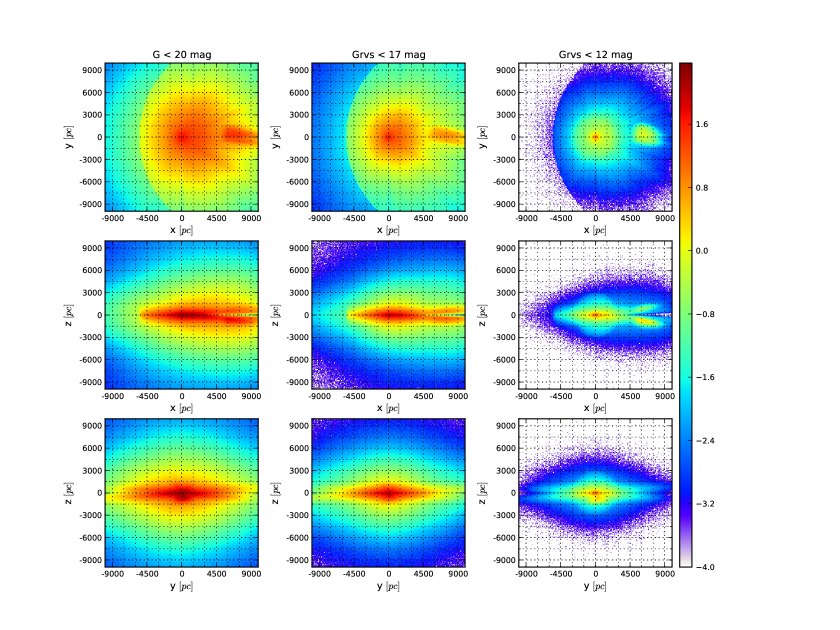
Figure 3.3: Distribution of star in heliocentric Cartesian coordinates ($G<20$): top (XY), side (XZ) and front (YZ) perspectives. Color scale indicates the $\log_{10}$ of the number of stars per square parsec.

Figure 3.4: $G$ distribution split by stellar population. It is worth noting that the bump for the bulge is due to the red clump, which is seen at I=15 in Baade’s window.

3.3 Star classification

As expected, the most abundant group of stars belong to the main sequence class (69%), followed by sub-giants (15%) and giants (14%). The complete star luminosity classification is given in table 3.3.

The star distribution as a function of $G$ can be found in figure 3.5. Main sequence stars present the biggest exponential increase, relatively similar to sub giants. The population of white dwarfs increases significantly starting at magnitude $G=14$. It is also interesting how supergiants decrease in number because they are intrinsically so bright and the peak that bright giants present at $G=14.5$. For both of them, the decrease corresponds mainly to the distance of the edge of the disc in the Galactic plane.

Table 3.3: Luminosity class of generated stars. Percentages have been calculated over the total number of stars for each respective column.

Luminosity class	G ¡ 20 mag	Grvs ¡ 17 mag	Grvs ¡ 12 mag
supergiant	0.00%	0.01%	0.07%
Bright giant	0.81%	2.18%	11.01%
Giant	14.47%	28.38%	62.71%
Sub-giant	15.08%	14.38%	10.32%
Main sequence	69.40%	54.82%	15.76%
Pre-main sequence	0.18%	0.20%	0.08%
White dwarf	0.05%	0.01%	0.03%
Others	0.01%	0.02%	0.02%
Total	1,100,000,000	390,000,000	13,000,000

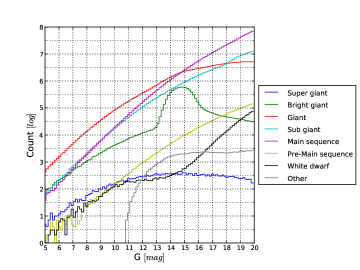
Figure 3.5: Star distribution split by luminosity class for $G<20$.

The spectral classification of stars (table 3.4) shows that G types are the most numerous (38%), followed by K types (28%) and F types (23%).

Table 3.4: Spectral types of generated stars. Percentages have been calculated over the total number of stars for each respective column.

Spectral type	G ¡ 20 mag	Grvs ¡ 17 mag	Grvs ¡ 12 mag
O	¡0.01%	¡0.01%	¡0.01%
B	0.26%	0.50%	0.88%
A	1.85%	3.30%	4.84%
F	23.13%	22.94%	13.83%
G	38.28%	31.58%	15.46%
K	27.68%	32.23%	41.75%
M	7.75%	6.78%	11.38%
L	¡0.01%	¡0.01%	¡0.01%
WR	¡0.01%	¡0.01%	0.01%
AGB	0.91%	2.50%	11.37%
Other	0.09%	0.07%	0.33%
Total	1,100,000,000	390,000,000	13,000,000

Considering the temperature and magnitude relation, HR diagrams have been generated (figure 3.6). Disc population represents the most complete one in terms of luminosity classes and spectral types distribution. The thin disc sequence of AGB stars going roughly from -4 to +17 in Mv is due to the heavy internal reddening of this population in visual bands. Isochrones can be clearly identified for thick disc, spheroid and bulge populations because they are assumed single burst generation. Additionally, all populations present a fraction of the white dwarfs generated by the model.

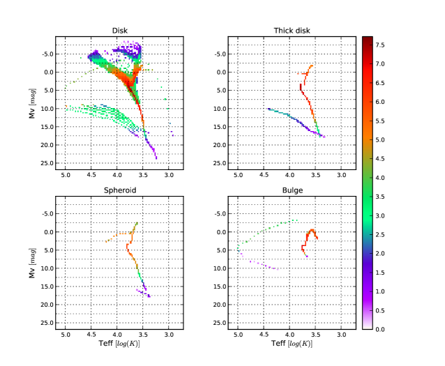
Figure 3.6: HR Diagram of stars split by population (left to right, top down): thin disc, thick disc, spheroid and bulge. Color scale indicates the $\log_{10}$ of the number of stars per 0.025 $\log\left(K\right)$ and 0.37 mag.

From the population perspective (figure 3.7), its is natural that bulge stars are concentrated at smaller parallaxes (bigger distances) while the rest increases from the sun position until the magnitude limit is reached and only brighter stars can be observed.

On the other hand, from a spectral type perspective, figure 3.8 presents the different parallax distributions for each type. Concrete numbers can be found in table 3.5 for specific parallaxes 240 $\mu$as, 480 $\mu$as and 960 $\mu$as which correspond to distances 4167 pc, 2083 pc and 1042 pc.

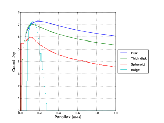
Figure 3.7: Stellar parallax split by populations

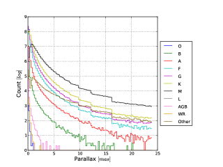
Figure 3.8: Stellar parallax split by spectral type

Table 3.5: Number of stars for each spectral type at different parallaxes. Percentages have been calculated over totals per spectral type, which can be deduced from table 3.4.

Spectral type	$\pi>240\mu$as	$\pi>480\mu$as	$\pi>960\mu$as
O	30.25%	1.54%	0.31%
B	38.38%	4.69%	0.99%
A	45.61%	9.87%	2.33%
F	35.06%	8.07%	1.74%
G	44.52%	11.48%	2.46%
K	70.61%	34.28%	7.94%
M	92.75%	90.50%	62.09%
L	0.00%	0.00%	0.00%
WR	27.98%	1.89%	0.23%
AGB	0.05%	0.01%	¡0.01%
Other	71.56%	64.73%	57.53%
Total	570,000,000	250,000,000	90,000,000

As mentioned in the introduction, the RVS instrument will be able to measure abundances of key chemical elements (e.g. Ca, Mg and Si) for stars up to $G_{\mathrm{RVS}}=12$. Metallicities and its relation to the abundances of alpha elements is presented in figure 3.9 split by population. Alpha element abundances are mostly reliable except at metallicity larger than 0.5, due to the formulation which is extrapolated. It will be corrected in a future version.

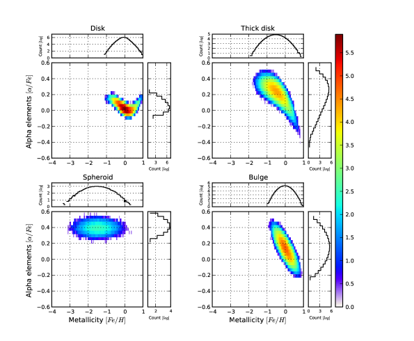
Figure 3.9: Metallicity - alpha elements relation for $G_{\mathrm{RVS}}<12$. Color scale indicates the $\log_{10}$ of the number of stars per 0.05 $\left[Fe/H\right]$ and 0.04 $\left[\alpha/Fe\right]$.

3.4 Kinematics

Proper motion of stars and radial velocity are represented in figure 3.10. Means are located at $\mu_{\alpha}\cos\left(\delta\right)=-1.95$ mas/year and $\mu_{\delta}=-2.78$ mas/year, which are affected by the motion of the solar local standard of rest.

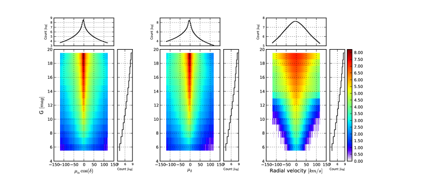
Figure 3.10: Proper motion of stars $\mu_{\alpha}cos\delta$, $\mu_{\delta}$ and radial velocity $V_{R}$. Color scale indicates the $\log_{10}$ of the number of stars per 2.4 mas/year (km/s in case of $V_{R}$) and 1.0 mag.

Older stars, which present poorest metallicities, tend to have lowest velocities on the V axis compared to the solar local standard of rest (figure 3.11) following the so-called asymmetric drift. The approximate mean V velocities are -48 km s^-1 for the thin disc, -98 km s^-1 for the thick disc, -243 km s^-1 for the spheroid and -116 km s^-1 for the bulge.

Figure 3.11: Metallicity and V axis velocity relation split by population (left to right, top down): thin disc, thick disc, spheroid and bulge. Color scale indicates the $\log_{10}$ of the number of stars per 0.05 $\left[Fe/H\right]$ and 6 km/s.

3.5 Variable stars

From the total amount of 1,600,000,000 individual stars generated by the model, ~1.8% are variable stars (of the variable types included in the Universe Model). They are composed by 6,800,000 single stars (~25% over total variable stars) with magnitude G less than 20 (observable by Gaia if their maximum magnitude is reached at least once during the mission) and 21,000,000 stars in multiple system (~75%). However, as explained in section 3.1, this last group is formed by stars that have magnitude G less than 20 as a system but, in some cases, its isolated components can have magnitude G superior to 20 and won’t be individually detectable by Gaia.

Again, only taking into consideration magnitude G and ignoring the angular separation of multiple systems, Gaia could be able to observe up to 21,500,000 variable stars in single and multiple systems (~2% over total individually observable stars exposed in section 3.1).

Regarding radial velocities, they will be measurable for 16,000,000 variable stars with $G_{\mathrm{RVS}}<17$, while metallicities will be available for 2,000,000 variable stars (~1%) with $G_{\mathrm{RVS}}<12$ (see table 3.6).

Table 3.6: Overview of variable stars. Percentages have been calculated over the total variable stars.

Stars	G ¡ 20 mag	Grvs ¡ 17 mag	Grvs ¡ 12 mag
Single variable stars	24.52%	25.79%	28.39%
Variable stars in multiple systems	75.48%	74.21%	71.61%
$\Rightarrow$ In binary systems	55.74%	52.65%	38.49%
$\Rightarrow$ Others (ternary, etc.)	19.73%	21.55%	33.12%
Total variable stars	28,000,000	19,000,000	2,700,000
Individually observable	21,500,000	16,000,000	2,000,000
With planets	2.09%	2.64%	2.09%

By variability type, $\delta$ scuti are the most abundant representing the 49% of the variable stars, followed by semiregulars (42%) and microlenses (4.3%) as seen in table 3.7. However, microlenses are highly related to denser regions of the galaxy as shown in figure 3.12, and they can involve stars of any kind. The rest of variability types are strongly related to different locations in the HR diagram (figure 3.13).

Table 3.7: Stars distribution by variability type.

Variability type	G ¡ 20 mag	Grvs ¡ 17 mag	Grvs ¡ 12 mag
ACV	0.61%	0.52%	0.18%
Flaring	1.46%	0.49%	0.01%
RRab	0.37%	0.34%	0.02%
RRc	0.09%	0.09%	0.01%
ZZceti	0.12%	¡0.01%	¡0.01%
Be	2.15%	2.02%	0.87%
Cepheids	0.03%	0.04%	0.11%
Classical novae	0.05%	0.06%	0.19%
$\delta$ scuti	48.57%	41.01%	14.11%
Dwarf novae	¡0.01%	¡0.01%	0.00%
Gammador	0.09%	0.01%	¡0.01%
Microlens	4.27%	1.87%	0.91%
Mira	0.19%	0.24%	0.91%
$\rho$ Ap	0.05%	0.04%	0.01%
Semiregular	41.94%	53.27%	82.6%
Total	21,500,000	16,000,000	2,000,000

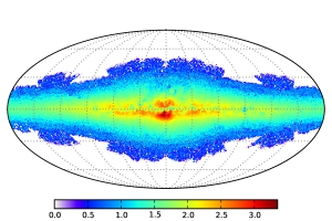
Figure 3.12: Sky distribution of microlenses that could take place during the 5 years of the mission. Color scale indicates the $\log_{10}$ of the number of microlenses per square degree.

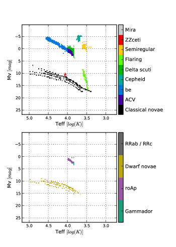
Figure 3.13: HR diagram split by variability type.

3.6 Binary stars

As seen in section 3.1, the model has generated 410,000,000 binary systems. Therefore about 820,000,000 stars have been generated but it is important to remark that not all of them will be individually observable by Gaia. Some systems may have components with magnitude G fainter than 20 (although the integrated magnitude is brighter) and others may be so close together that they cannot be resolved (although they can be detected by other means).

The majority of the primary stars are from the main sequence (67%), being the most popular combination a double main sequence star system (62%). Sub-giants and giants as primary coupled with a main sequence star are the second and third most probable systems (16% and 14% respectively). In general terms, the distribution is coherent with star formation and evolution theories (e.g. supergiants are not accompanied by white dwarfs), see table 3.8.

Table 3.8: Binary stars classified depending on the luminosity class combination (only binary systems whose integrated magnitude is G¡20). Values are in percentage.

	Supergiant	Bright Giant	Giant	Sub-giant	Main sequence	White dwarf	Others	Total per primary
Supergiant	0.0000	0.0001	0.0001	0.0004	0.0021	0.0000	0.0000	0.0028
Bright giant	0.0000	0.0022	0.0140	0.0154	0.1487	0.0015	0.0000	0.1819
Giant	0.0000	0.2933	0.5933	0.4997	12.7477	0.7229	0.0072	14.8641
Sub-giant	0.0001	0.5135	0.6916	0.5429	16.1521	0.0000	0.0100	17.9101
Main sequence	0.0001	0.4990	1.1328	0.0657	63.0344	1.8421	0.0000	66.5743
White dwarf	0.0000	0.0019	0.0059	0.0043	0.4258	0.0280	0.0000	0.4659
Others	0.0000	0.0001	0.0001	0.0000	0.0009	0.0001	0.0000	0.0011
Total per secondary	0.0002	1.3101	2.4378	1.1283	92.5118	2.5946	0.0172

The magnitude difference versus angular separation between components is shown in figure 3.14. While main sequence pairs should produce only negative magnitude differences, the presence of white dwarf primaries with small red dwarf companions produce the asymmetrical shape of the figure (recalling that ”primary” here means the more massive). To give a hint of the angular resolution capabilities of Gaia, we can assume it at first step as nearly diffraction-limited and correctly sampled with pixel size $\approx 59$ mas. Figure 3.14 thus shows that a small fraction only of binaries with moderate magnitude differences will be resolved.

The mean separation of binary systems is $30$ AU and they present a mean orbital period of about 250 years (figure 3.15). While only pairs with periods smaller than a decade may have their orbit determined by Gaia, a significative fraction of binaries will be detected through the astrometric “acceleration” of their motion.

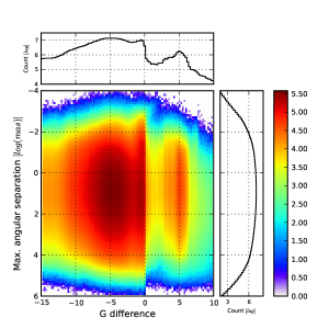
Figure 3.14: G difference and angular separation relation for binaries. Color scale indicates the $\log_{10}$ of the number of binaries per 0.25 difference in magnitude and $6\,\log\left(mas\right)$.

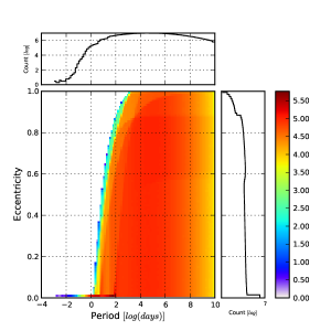
Figure 3.15: Period - Eccentricity relation for binaries. Color scale indicates the $\log_{10}$ of the number of binaries per 0.01 difference in eccentricity and $0.13\log\left(\mathrm{days}\right)$.

3.7 Stars with planets

A total number of 34,000,000 planets have been generated and associated to 27,500,000 single stars (~2.6% over total individually observable stars exposed in section 3.1), implying that 25% of the stars have been generated with two planets (table 3.9). No exoplanets are associated to multiple systems in this version of the model.

Table 3.9: Overview of stars with planets

Stars	G ¡ 20 mag	Grvs ¡ 17 mag	Grvs ¡ 12 mag
Total stars with planets	27,500,000	9,000,000	182,000
$\Rightarrow$ Stars with one planet	75.00%	74.99%	74.93%
$\Rightarrow$ Stars with two planets	25.00%	25.01%	25.07%
Total number of planets	34,000,000	11,000,000	228,000

The majority of star with planets belong to the main sequence (66%), followed by giants (17%) and sub-giants (16.8%) as shown in table 3.10. Only 8% of stars have a planet that produces eclipses.

Table 3.10: Luminosity class of stars with planets

Luminosity class	G ¡ 20 mag	Grvs ¡ 17 mag	Grvs ¡ 12 mag
Supergiant	¡0.01%	0.01%	0.14%
Bright giant	0.18%	0.46%	2.50%
Giant	17.04%	34.05%	65.01%
Sub-giant	16.81%	14.07%	11.91%
Main sequence	65.72%	51.19%	20.36%
Pre-main sequence	0.20%	0.22%	0.08%
White dwarf	0.03%	¡0.01%	¡0.01%
Others	¡0.01%	¡0.01%	¡0.01%
Total	27,500,000	9,000,000	182,000

On the other hand, stars with solar or higher metallicities present a bigger probability of having a planet than stars poorer in metals (figure 3.16).

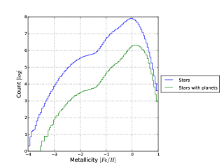
Figure 3.16: Metallicity distribution of stars with planets.

Finally, 77% of stars with planets belong to the thin disc population, while 11% are in the bulge, 11% in the thick disc and 0.4% in the spheroid (figure 3.17).

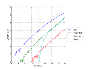
Figure 3.17: G distribution of stars having planets split by population.

3.8 Extragalactic objects

Apart from the stars presented in the previous sections, the model generates 8,800,000 additional stars that belong to the Magellanic Clouds. Again, the most abundant spectral type are G stars (46%), followed by K types (33%) and A types (17%). There are no F type stars reachable by Gaia, because the magnitude cut at the cloud distance selects only the upper part of the HR diagram including massive stars on the blue side, and late type giants and supergiants on the red side.

Table 3.11: Overview of extragalactic objects

Stars	G ¡ 20 mag	Grvs ¡ 17 mag	Grvs ¡ 12 mag
Stars in LMC	7,550,000	1,039,000	5,600
Stars in SMC	1,250,000	161,000	950
Unresolved galaxies	38,000,000	3,000,000	4,320
QSO	1,000,000	5,200	11
Supernovae	50,000	-	-

Table 3.12: Spectral types of stars from LMC/SMC

Spectral type	G ¡ 20 mag	Grvs ¡ 17 mag	Grvs ¡ 12 mag
O	0.25%	0.17%	0.39%
B	3.24%	3.40%	1.85%
A	17.20%	5.01%	4.83%
F	0.00%	0.00%	0.00%
G	45.98%	23.16%	55.19%
K	32.62%	64.82%	35.33%
M	0.71%	3.44%	2.41%
Total	8,800,000	1,200,000	6,600

Regarding unresolved galaxies, 38,000,000 have been generated. However due to the on board thresholding algorithm optimized for point sources, a significant fraction of these galaxies will not have their data transfered to Earth. Gaia will be able to measure radial velocities for only 8% and metal abundances for 0.01% of them. The most frequent galaxy type are spirals (58% considering Sa, Sb, Sc, Sd, Sbc), followed by irregulars (25%) and ellipticals (13% adding E2 and E-S0) as seen in table 3.13.

Table 3.13: Galaxies by type. Percentages calculated over total galaxies (table 3.11).

Galaxies	G ¡ 20 mag	Grvs ¡ 17 mag	Grvs ¡ 12 mag
E2	6.36%	10.24%	10.51%
E-S0	7.03%	11.67%	12.85%
Sa	7.51%	10.55%	10.05%
Sb	9.21%	12.39%	13.70%
Sc	10.21%	8.50%	8.08%
Sd	22.08%	17.08%	15.00%
Sbc	9.21%	12.35%	13.73%
Im	24.77%	15.46%	14.44%
QSFG	3.61%	1.76%	1.64%

Additionally, 1,000,000 quasars have been generated and the model predicts 50,000 supernovas that will occur during the 5 years of mission, being 77% of them from Ia type (table 3.14).

Table 3.14: Supernovae types. Percentages calculated over 50,000 supernovas.

Supernovae types
Ia	76.74%
Ib/c	7.36%
II-L	14.24%
II-P	1.65%

The sky distribution of these three types of objects is shown in figure 3.18.

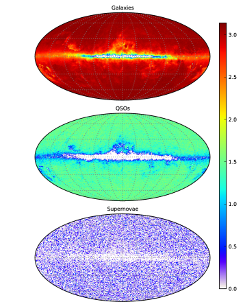
Figure 3.18: Total sky distribution of unresolved galaxies, quasars and supernovae. Color scale indicates the $\log_{10}$ of the number of objects per square degree.

Regarding redshifts, galaxies go up to $z\sim 0.75$, while the most distant quasars are at $z\sim 5$. Magnitudes also present a different pattern depending on the type of object as shown in figure 3.19.

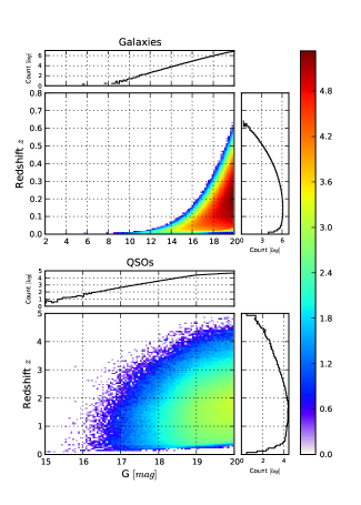
Figure 3.19: Redshift and G relation for galaxies and QSOs. Color scale indicates the $\log_{10}$ of the number of objects per 0.05 mag and 0.05 redshift difference.

4 Conclusions

Gaia will be able to provide a much more precise and complete view of the Galaxy than its predecessor Hipparcos, representing a large increase in the total number of stars (table 4.1) and the solar neighbourhood (table 4.2).

Table 4.1: Comparison of Hipparcos and Gaia characteristics and the predicted number of stars, variables and binaries presented in this study.
* Includes stars which may not be resolved due to its angular separation and Gaia resolution power.

	Hipparcos	Gaia
Number of stars	118,218	$1,100,000,000{}^{*}$
Mean sky density (per square degree)	~ 3	~ 30.425
Limiting magnitude	V ~ 12.4 mag	V ~ 20 – 25 mag
Median astrometric precision	0.97 mas (V¡9)	~ 10$\mu$ as (V=15)
Possibly variable	11,597	$21,500,000^{*}$
Suspected double systems	23,882	$410,000,000^{*}$

Table 4.2: Number of nearby stars (within 25 pc) detected by Hipparcos compared with the predicted number of stars in the universe model

Distance (pc)		Stars
Min.	Max.	Hipparcos (V ¡ 9)	Gaia (G ¡ 20)
20	25	1,126	4,563
10	20	1,552	1,784
5	10	257	927
0	5	61	706
0	25	2,996	7,980

The Gaia Universe Model, and other population synthesis models in general, can be useful tools for survey preparation. In this particular case, it has been possible to obtain a general idea of the numbers, percentages and distribution of different objects and characteristics of the environment that Gaia can potentially observe and measure.

Additionally, the analysis of the snapshot has facilitated the detection of several aspects to be improved. Therefore, it has been a quite fruitful quality assurance process from a scientific point of view.

Looking forward, the next reasonable step would be to reproduce the same analysis but taking into consideration the instrument specifications and the available error models. By convolving it with the idealized universe model presented in this paper, it will be possible to evaluate the impact of the instrumental effects on the actual composition of the Gaia catalogue. In the mean time the simulated catalogue presented in this paper will be publicly available through the ESA Gaia Portal at http://www.rssd.esa.int/gaia/.

NOTE: Internal referred documents from the Gaia mission can be found at http://www.rssd.esa.int/index.php?project=GAIA&page=Library_Livelink

References

- Arenou (2010) Arenou, F. 2010, The simulated multiple stars, Tech. rep., Observatoire de Paris-Meudon, GAIA-C2-SP-OPM-FA-054
- Arenou (2011) Arenou, F. 2011, in American Institute of Physics Conference Series, Vol. 1346, International Workshop Double and Multiple Stars: Dynamics, Physics, and Instrumentation, ed. J. A. Docobo, V. S. Tamazian, & Y. Y. Balega, 107–121
- Baraffe et al. (2003) Baraffe, I., Chabrier, G., Barman, T. S., Allard, F., & Hauschildt, P. H. 2003, aap, 402, 701
- Belokurov & Evans (2003) Belokurov, V. A. & Evans, N. W. 2003, mnras, 341, 569
- Bergbush & VandenBerg (1992) Bergbush, P. & VandenBerg, D. 1992, ApJS, 81, 163
- Bertin (2009) Bertin, E. 2009, memsai, 80, 422
- Bienayme et al. (1987) Bienayme, O., Robin, A. C., & Crézé, M. 1987, Astronomy and Astrophysics (ISSN 0004-6361), 180, 94
- Cardelli et al. (1989) Cardelli, J. A., Clayton, G. C., & Mathis, J. S. 1989, ApJ, 345, 245
- Chabrier (1999) Chabrier, G. 1999, ApJ, 513, L103
- Cox et al. (2000) Cox, A. N., Becker, S. A., & Pesnell, W. D. 2000, Theoretical Stellar Evolution, ed. Cox, A. N., 499
- Dollet (2004) Dollet, C. 2004, PhD Thesis, Tech. rep., Université de Nice
- Drimmel et al. (2003) Drimmel, R., Cabrera-Lavers, A., & Lopez-Corredoira, M. 2003, Astron.Astrophys., 409:205-216,2003
- Eyer et al. (2005) Eyer, L., Robin, A., Evans, D. W., & Reylé, C. 2005, Implementation of variable stars in the Galactic model. I. General concept, Tech. rep., Observatoire de Genève, VSWG-LE-002
- Feast et al. (1989) Feast, M. W., Glass, I. S., Whitelock, P. A., & Catchpole, R. M. 1989, mnras, 241, 375
- Fioc & Rocca-Volmerange (1997) Fioc, M. & Rocca-Volmerange, B. 1997, A&A, 326, 950
- Fioc & Rocca-Volmerange (1999) Fioc, M. & Rocca-Volmerange, B. 1999, A&A, 344, 393
- Fischer & Valenti (2005) Fischer, D. A. & Valenti, J. 2005, apj, 622, 1102
- Gomez et al. (1997) Gomez, A. E., Grenier, S., Udry, S., et al. 1997, in ESA Special Publication, Vol. 402, ESA Special Publication, 621–624
- Greggio & Renzini (1983) Greggio, L. & Renzini, A. 1983, A&A, 118, 217
- Han (2008) Han, C. 2008, apj, 681, 806
- Haywood (2008) Haywood, M. 2008, MNRAS, 388, 1175
- Haywood et al. (1997a) Haywood, M., Robin, A. C., & Crézé, M. 1997a, Astronomy and Astrophysics (ISSN 0004-6361), 320, 428
- Haywood et al. (1997b) Haywood, M., Robin, A. C., & Crézé, M. 1997b, Astronomy and Astrophysics (ISSN 0004-6361), 320, 440
- Hunter (2007) Hunter, J. D. 2007, Computing In Science & Engineering, 9, 90
- Jaschek et al. (1988) Jaschek, C., Jaschek, M., Egret, D., & Andrillat, Y. 1988, A&A, 192, 285
- Jordi et al. (2010) Jordi, C., Gebran, M., Carrasco, J. M., et al. 2010, A&A, 523, A48+
- Kochukhov (2007) Kochukhov, O. 2007, Communications in Asteroseismology, 150, 39
- Kovalevsky (2003) Kovalevsky, J. 2003, aap, 404, 743
- Kowalski et al. (2009) Kowalski, A. F., Hawley, S. L., Hilton, E. J., et al. 2009, aj, 138, 633
- Krone-Martins et al. (2008) Krone-Martins, A. G. O., Ducourant, C., Teixeira, R., & Luri, X. 2008, in IAU Symposium, Vol. 248, IAU Symposium, ed. W. J. Jin, I. Platais, & M. A. C. Perryman, 276–277
- Kunszt et al. (2001) Kunszt, P. Z., Szalay, A. S., & Thakar, A. R. 2001, in Mining the Sky, ed. A. J. Banday, S. Zaroubi, & M. Bartelmann, 631–+
- Kurtz (1982) Kurtz, D. W. 1982, mnras, 200, 807
- Mignard (2005) Mignard, F. 2005, in ESA Special Publication, Vol. 576, The Three-Dimensional Universe with Gaia, ed. C. Turon, K. S. O’Flaherty, & M. A. C. Perryman, 5–+
- Molinaro et al. (2011) Molinaro, R., Ripepi, V., Marconi, M., et al. 2011, MNRAS, 413, 942
- Ojha et al. (1996) Ojha, D., Bienayme, O., Robin, A., Crézé, M., & Mohan, V. 1996, A&A, 311, 456
- Ojha et al. (1999) Ojha, D. K., Bienaymé, O., Mohan, V., & Robin, A. C. 1999, A&A, 351, 945
- Paczynski (1986) Paczynski, B. 1986, ApJ, 304, 1
- Perryman et al. (2001) Perryman, M. A. C., de Boer, K. S., Gilmore, G., et al. 2001, Astron.Astrophys., 369:339-363,2001
- Reid et al. (2002) Reid, I. N., Gizis, J. E., & Hawley, S. L. 2002, aj, 124, 2721
- Reylé et al. (2009) Reylé, C., Marshall, D. J., Robin, A. C., & Schultheis, M. 2009, aap, 495, 819
- Reylé et al. (2007) Reylé, C., Robin, A., Arenou, F., & Grux, E. 2007, Universe Model Interface Control Document, Tech. rep., Obs. de Besançon, Obs. de Paris-Meudon, GAIA-C2-SP-LAOB-CR-001
- Robin et al. (1992) Robin, A. C., Crézé, M., & Mohan, V. 1992, ApJ, 400, L25
- Robin et al. (2003) Robin, A. C., Reylé, C., Derriére, S., & Picaud, S. 2003, Astronomy and Astrophysics (ISSN 0004-6361), 409, 523
- Schechter (1976) Schechter, P. 1976, apj, 203, 297
- Slezak & Mignard (2007) Slezak, E. & Mignard, F. 2007, A realistic QSO Catalogue for the Gaia Universe Model, Tech. rep., Observatoire de la Côte d’Azur, GAIA-C2-TN-OCA-ES-001-1
- Sozzetti et al. (2009) Sozzetti, A., Torres, G., Latham, D. W., et al. 2009, apj, 697, 544
- Stift & Alecian (2009) Stift, M. J. & Alecian, G. 2009, mnras, 394, 1503
- Tabachnik & Tremaine (2002) Tabachnik, S. & Tremaine, S. 2002, mnras, 335, 151
- Tanga (2011) Tanga, P. 2011, in EAS Publications Series, Vol. 45, EAS Publications Series, 225–230
- Tsalmantza et al. (2009) Tsalmantza, P., Kontizas, M., Rocca-Volmerange, B., et al. 2009, A&A, 504, 1071
- van der Hucht (2001) van der Hucht, K. A. 2001, New Astronomy Review, 45, 135
- Véron-Cetty & Véron (2006) Véron-Cetty, M.-P. & Véron, P. 2006, aap, 455, 773
- Wood (1992) Wood, M. A. 1992, ApJ, 386, 539
- Zorec & Briot (1997) Zorec, J. & Briot, D. 1997, A&A, 318, 443