An order-$N$ electronic structure theory with generalized eigen-value equations and its application to a ten-million-atom system

Abstract

A linear-algebraic theory called ‘multiple Arnoldi method’ is presented and realizes large-scale (order-$N$) electronic structure calculation with generalized eigen-value equations. A set of linear equations, in the form of $(zS-H)\bm{x}=\bm{b}$, are solved simultaneously with multiple Krylov subspaces. The method is implemented in a simulation package ELSES (http://www.elses.jp) with tight-binding-form Hamiltonians. A finite-temperature molecular dynamics simulation is carried out for metallic and insulating materials. A calculation with $10^{7}$ atoms was realized by a workstation. The parallel efficiency is shown upto 1,024 CPU cores.

1 Introduction

Large-scale electronic structure calculation, with $10^{3}$ atoms or more, plays a crucial role in nano science and is realized by an order-$N$ theory, in which the computational cost is proportional to the system size. References on the order-$N$ electronic structure theory can be found in a recent paper. [1] In this paper, a method, called ‘multiple Arnoldi method’, is presented for generalized eigen-value equations, or large-scale electronic structure theory with non-orthogonal (atomic) bases. The method is applicable both to metal and insulator and the molecular dynamics (MD) simulations were carried out for upto ten-million-atom systems with tight-binding-form Hamiltonians. The present method is a theoretical extension of a previous one, the diagonalization method in the Krylov subspace, [2, 3], since the present method will be reduced to the previous one in the case with orthogonal bases.

This paper is organized as follows; The theory is summarized in Sec. 2. In Sec. 3, numerical examples appear and the method is compared with several existing ones with non-orthogonal bases. [1] The summary is given in Sec. 4.

In this paper, the $j$-th unit vector is denoted as $\bm{e}_{j}\equiv(0,0,0\ldots,1_{j},0,0,0,\ldots,0_{M})^{\rm T}$. The inner product between the two vectors of $\bm{f}\equiv(f_{1},f_{2},\ldots)^{\rm T},\bm{g}\equiv(g_{1},g_{2},\ldots)^{\rm T}$ is written as $\bm{f}^{\rm T}\bm{g}\equiv\sum_{i}f_{i}g_{i}$. The unit matrix is denoted as $I$. The representation with atomic orbitals is considered and the suffix $i$ for a component of a vector indicates the composite suffix for atom and orbital ($s,p_{x},p_{y},p_{z},...$).

2 Theory

A key concept of the present method is the Krylov subspace that is defined as a linear (Hilbert) space of

$$K_{\nu}(A;\bm{b})\equiv{\rm span}\{\bm{b},A\bm{b},A^{2}\bm{b},\ldots,A^{\nu-1}\bm{b}\}$$ (1)

with a given square matrix $A$ and a given vector $\bm{b}$. Krylov subspace is a common mathematical foundation for iterative linear algebraic algorithms, such as the conjugate-gradient (CG) algorithm.

A generalized eigen-value equation is written as

$$H\bm{\phi}_{k}=\varepsilon_{k}S\bm{\phi}_{k}.$$ (2)

Here the Hamiltonian and overlap matrices are denoted as $H$ and $S$, respectively. They are sparse real-symmetric $M\times M$ matrices and $S$ is positive definite. The eigen levels and vectors are denoted as $\varepsilon_{k}$ and $\bm{\phi}_{k}$, respectively.

A basic equation for large-scale electronic structure theory is the set of linear equations

$$(zS-H)\bm{x}_{j}=\bm{e}_{j}$$ (3)

among the unit vectors $\{\bm{e}_{j=1},\bm{e}_{2},\bm{e}_{3},....,\bm{e}_{M}\}$. A matrix element of the Green’s function, $G\equiv(zS-H)^{-1}$, [4] is given as $G_{ij}=\bm{e}_{i}^{\rm T}\bm{x}_{j}$.

In the present method, the solution of Eq.(3) is given within the multiple Krylov subspace of

$${\cal L}_{\nu}^{(j)}=K_{p}(H;\bm{e}_{j})\oplus K_{q}(H;S^{-1}\bm{e}_{j}),$$ (4)

where $p,q$ are positive integers and $\nu\equiv p+q$. The dimension of the subspace, $\nu$, is chosen to be much smaller than that of the original matrices. The case with $q=0$ is the generalized Arnoldi method in Ref. [1]

The two initial vectors of $\bm{e}_{j}$ and $\bm{s}_{j}\equiv S^{-1}\bm{e}_{j}$ in Eq. (4) satisfy a ‘duality’ relation of $\bm{e}_{j}^{\rm T}S\bm{s}_{j}=1$. A formulation with the dual vectors reduces An efficient numerical treatment of $S^{-1}\bm{e}_{j}$ is required for a large-scale calculation, since the explicit matrix-inversion procedure of $S$ is costful, as the matrix-diagonalization procedure. In the present method, the vector of $\bm{s}_{j}:=S^{-1}\bm{e}_{j}$ is calculated by an inner CG loop, in which the linear equation of $S\bm{s}_{j}=\bm{e}_{j}$ is solved iteratively with the standard CG method. This inner loop converges fast, typically with $\nu_{\rm CG}=10-30$ iterations, since the overlap matrix is sparse and nearly equal to the unit matrix $(S\approx I)$. [1]

The whole procedures are carried out in the following two stages. First, the bases of the subspaces

$${\cal L}_{\nu}^{(j)}\equiv{\rm span}\{\bm{u}_{1}^{(j)},\bm{u}_{2}^{(j)},\ldots,\bm{u}_{\nu}^{(j)}\},$$ (5)

are generated so as to satisfy the ‘$S$-orthogonality’ ($\bm{u}_{m}^{(j){\rm T}}S\bm{u}_{n}^{(j)}=\delta_{mn}$); With a given initial vector of $\bm{l}_{1}:=\bm{e}_{j}$, the $n$-th basis ($\bm{u}_{n}$), for $n\geq 1$ and $n\neq p+1$, is generated in the following three procedures;

$$\bm{u}_{n} := \frac{\bm{l}_{n}}{\sqrt{\bm{l}_{n}^{t}S\bm{l}_{n}}}$$ (6)

$$\bm{k}_{n} := H\bm{u}_{n}$$ (7)

$$\bm{l}_{n+1} := \bm{k}_{n}-\sum_{m=1}^{n}\bm{u}_{m}q_{mn}$$ (8)

with $q_{mn}\equiv\bm{u}_{m}^{t}S\bm{k}_{n}$. The modified Gram-Schmidt procedure appear in Eq. (8), so as to satisfy the ‘S-orthogonality’ of $\bm{u}_{m}^{t}S\bm{k}_{n+1}=0$ for $m=1,2,\ldots,n$. For $n=p+1$, Eq. (7) is replaced by

$$\bm{k}_{p+1}:=S^{-1}\bm{e}_{j}.$$ (9)

The $S^{-1}$-vector multiplication in Eq. (9 ) is realized by the inner CG loop explained above.

Second, subspace eigen vectors $\bm{v}_{\alpha}^{(j)}$ ($\subset{\cal L}_{\nu}^{(j)}$)

$$\bm{v}^{(j)}_{\alpha}=\sum_{n}^{\nu}C_{n\alpha}^{(j)}\bm{u}_{n}^{(j)}$$ (10)

and subspace eigen levels $\varepsilon^{(j)}_{\alpha}$ are introduced so that the residual vector $\bm{r}^{(j)}_{\alpha}\equiv(H-\varepsilon^{(j)}_{\alpha}S)\bm{v}^{(j)}_{\alpha}$ is orthogonal to the subspace ($\bm{r}_{\alpha}^{(j)}\perp{\cal L}_{\nu}^{(j)}$). The above principle is known as Galerkin principle in numerical analysis. [6] Consequently, a standard eigen-value equation appears with a reduced ($\nu\times\nu$) Hamiltonian matrix of $(H^{(j)})_{mn}\equiv\bm{u}_{m}^{(j){\rm T}}H\bm{u}_{n}^{(j)}$. The derived eigen-value equation is solved, so as to determine $\varepsilon^{(j)}_{\alpha}$ and $C_{n\alpha}^{(j)}$.

The solution vector is determined as

$$\bm{x}_{j}(z):=G^{(j)}(z)\bm{e}_{j}$$ (11)

where the matrix $G^{(j)}$, called ‘subspace Green’s function’, is defined as

$$G^{(j)}\equiv\sum_{\alpha}\frac{\bm{v}_{\alpha}^{(j)}\bm{v}_{\alpha}^{(j){\rm T}}}{z-\varepsilon_{\alpha}^{(j)}}.$$ (12)

The above calculation will be exact, when the subspace ${\cal L}_{\nu}^{(j)}$ comes to the complete space ($\nu\rightarrow M$).

The density matrix and the energy density matrix

$$\rho_{ij} := \sum_{\alpha}^{\nu}f(\varepsilon^{(j)}_{\alpha})\bm{e}_{i}^{\rm T}\bm{v}^{(j)}_{\alpha}\bm{v}^{(j){\rm T}}_{\alpha}\bm{e}_{j}$$ (13)

$$\pi_{ij} := \sum_{\alpha}^{\nu}f(\varepsilon^{(j)}_{\alpha})\varepsilon^{(j)}_{\alpha}\bm{e}_{i}^{\rm T}\bm{v}^{(j)}_{\alpha}\bm{v}^{(j){\rm T}}_{\alpha}\bm{e}_{j}$$ (14)

are calculated where the occupation number $f(\varepsilon)$ is the Fermi-Dirac function with the given values of the temperature (level-broadening) parameter and the chemical potential $\mu$. The chemical potential is determined by the bisection method, so that the total electron number is the correct one.

The electronic structure energy ($E_{\rm elec}$) and its derivative with respect to the $K$-th atom position ($\bm{F}_{K}$) are required for a MD simulation. They are decomposed into the partial sums as

$$E_{\rm elec} \equiv {\rm Tr}[\rho H]=\sum_{j}E_{\rm elec}^{(j)}$$ (15)

$$\bm{F}_{K} \equiv -\frac{\partial E_{\rm elec}}{\partial\bm{R}_{K}}=\sum_{j}\bm{F}_{K}^{(j)},$$ (16)

where the partial sums are defined by

$$E_{\rm elec}^{(j)} \equiv \sum_{i}\rho_{ij}H_{ji}$$ (17)

$$\bm{F}_{K}^{(j)} \equiv -\sum_{i}\left\{\rho_{ij}\frac{\partial H_{ji}}{\partial\bm{R}_{K}}+\pi_{ij}\frac{\partial S_{ji}}{\partial\bm{R}_{K}}\right\}.$$ (18)

The components of $\rho_{ij}$ or $\pi_{ij}$ are required only for the selected $(i,j)$ pairs that satisfy $H_{ij}\neq 0$ or $S_{ij}\neq 0$, respectively. The value of $\bm{F}_{K}^{(j)}$ in Eq. (18) is contributed only within a local region where the atom positions of the $i$-th and $j$-th bases are equal to or near the $K$-th atom position ($\bm{R}_{K}$), because the value of $(\partial H_{ji}/\partial\bm{R}_{K})$ or $(\partial S_{ji}/\partial\bm{R}_{K})$ is non-zero only for the local region.

The calculation work flow is summarized as

$$\{\{\bm{u}_{n}^{(j)}\}\Rightarrow\{\bm{v}^{(j)}_{\alpha},\varepsilon^{(j)}_{\alpha}\}\}_{j}\Rightarrow({\rm bisection})\Rightarrow\mu$$ (19)

$$\Rightarrow \{f(\varepsilon^{(j)}_{\alpha})\}_{j}\Rightarrow\{\{\rho_{ij},\pi_{ij}\}\Rightarrow\{E_{\rm elec}^{(j)},\{F_{K}^{(j)}\}\}\}_{j}$$

where the procedures in a curly parenthesis $\{\cdot\cdot\cdot\cdot\}_{j}$ are carried out independently among the running index $j$, as a parallel computation. In the bisection procedure, the total electron number with a trial value of the chemical potential is summed up among the bases and the summation is parallelized with the basis index $j$.

Several calculations with the charge-self-consistent (CSC) formulation [7] were also carried out. At each MD step, an iterative loop is required for the self consistency of the change distribution. Since the overlap matrix is unchanged within the iterative loop, the inner CG loop for $S^{-1}\bm{e}_{j}$ is required only once at one MD step and gives a tiny fraction of the total computational cost.

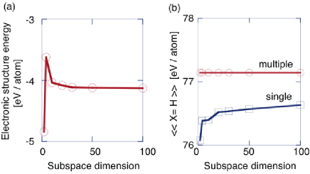
Figure 1: Numerical example of solid gold with 864 atoms. (a) The electronic structure energy in the multiple subspace method, calculated with the subspace dimension of $\nu=2,4,10,20,30,50,100$. (b) The estimated energy value from the whole spectrum in the multiple subspace method (red line) and in the single subspace method (blue line), calculated with the subspace dimension of $\nu=2,4,10,20,30,50,100$.

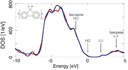
Figure 2: The density of states of an amorphous-like conjugated polymer (poly-(9,9 dioctyl-fluorene)), calculated by the present method (blue line) and by the exact diagonalization method (red line). The HO and LU levels are indicated by arrows. The HO and LU levels of benzene are also indicated by arrows. The inset shows the monomer unit with $R\equiv$ C₈H₁₇.

3 Examples and discussion

Several numerical examples are calculated by the multiple Arnoldi method. We choose $p=q=\nu/2$ ($\nu$ : even) in the following calculations, except where indicated, so as to investigate the examples, systematically among different values of the subspace dimension ($\nu$), with a significant contribution by the second term in Eq. (4).

Figure 1(a) shows the electronic structure energy $E_{\rm elec}$ for bulk gold with 864 atom. The tight-binding-form Hamiltonian in Ref. [8] was used and contains $s$, $p$ and $d$ orbitals. The electronic structure energy was calculated with the subspace dimensions of $\nu=2,4,10,20,30,50,100$. The calculated energy agrees for $\nu=30,50,100$ within deviations less than 0.01 eV per atom. In general, the use of the multiple Krylov subspaces ($p,q\geq 1$) reproduces several properties. (i) In the fully filled limit ($f(\varepsilon)\rightarrow 1$), a physical quantity is contributed by all the eigen states and is expressed by

$$\langle\langle X\rangle\rangle\equiv\sum_{k}\bm{\phi}_{k}^{\rm T}X\bm{\phi}_{k}={\rm Tr}[S^{-1}X].$$ (20)

with a real-symmetric matrix $X$. One can prove the fact that Eq. (20) holds exactly, if $q\geq 1$ (or $S^{-1}\bm{e}_{j}\subset{\cal L}^{(j)}$). [9] Figure  1(b) confirms the fact numerically in the case of $X=H$. (ii) One can also prove that the equivalence of the two expressions of the band structure energy (${\rm Tr}[\rho H]={\rm Tr}[\pi S]$) [1] holds exactly, if $p\geq 1$ (or $\bm{e}_{j}\subset{\cal L}^{(j)}$). The equivalence was confirmed numerically (not shown).

A MD simulation for a semiconducting system was carried out with $\nu=30$ for an amorphous-like structure of a conjugated polymer, poly-(9,9 dioctyl-fluorene) with 2076 atoms. [10] The simulation was carried out with the tight-binding Hamiltonian of a modified extended Hückel type in Ref. [11]. The results for the monomer and dimer agree reasonably to those by the ab initio calculation of Gaussian^(TM) with the B3LYP functional and the 6-311G(d,p) basis set. Detailed data by the present method are added here with those by the ab initio calculation in the parentheses; The valence band width $W$ and the band gap $\Delta$ are $W=18.5$ eV (18.3 eV) and $\Delta=4.25$ eV (4.91 eV) in the monomer and $W=19.0$ eV (18.8 eV) and $\Delta=3.58$ eV (4.10 eV) in the dimer. The two monomers in the dimer are twisted along the main chain and the twisting angle $\theta$ is $\theta=37.3^{\circ}$ (40.6 ^∘). As a technical detail in large-scale calculations, the real-space projection method was used and is explained in Appendix of Ref.  [3] In short, the Krylov subspace is generated by a Hamiltonian projected in real space, $H^{(j)}\equiv P^{(j)}HP^{(j)}$, instead of the original one $H$, where the projection operator $P^{(j)}$ projects a function onto the spherical region whose center is located at the atomic position of the $j$ th atomic basis. The projection radius is determined for each basis $\bm{e}_{j}$, so that the region contains $N_{\rm RP}$ atoms or more. The same technique is used also for the overlap matrix. The value of $N_{\rm RP}$ is an input parameter and is set to $N_{\rm RP}=100$.

Figure 2 shows the density of state (DOS), calculated from the Green’s function, for the amorphous-like conjugated polymer. The calculation of DOS requires a finer calculation conditions ($\nu$ = 300 and $N_{\rm RP}=1000$) than that for the density matrix, since the DOS profile is an energy resolved quantity. The result by the exact diagonalization method is also shown and one finds that the present method reproduces the overall spectrum precisely. Moreover, when the eigen levels are assumed to be non-degenerated, the calculated Green’s function can be decomposed into the contributions of individual eigen states and the individual eigen levels can be estimated. [12] For example, the highest-occupied (HO) and lowest occupied (LU) levels were estimated and are indicated by the arrows in Fig. 2. These values agree excellently, within less than 3 meV, with those in the exact diagonalization method. The agreement is also found on a couple of levels near the HO and LU levels. It is noteworthy that a state located near a band edge, such as HO and LU states, is reproduced with a smaller subspace dimension ($\nu$) than one located within the band, as a general property of the subspace theory. [13]

A MD simulation was carried out also for a gold nanowire, a metal. The same conditions of $\nu$ and $N_{\rm PR}$ were used as in the polymer simulation. The simulation by the present method reproduces the formation process of helical gold nanowire, as ones by the exact diagonalization method. [14, 15]

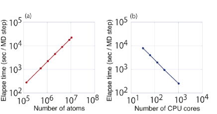
Figure 3: Calculation of the amorphous-like polymer. (a) Order-$N$ scaling property upto 10⁷ atoms. (b) Parallel efficiency with 10⁷ atoms upto 1,024 CPU cores.

A high computational efficiency is shown for the present method among calculations of the conjugated polymer. When the system with 2076 atoms was calculated by a work station with two six-core Xeon CPUs (X5650), the present method consumes 2.6 seconds per MD step and is faster, approximately by ten times, than the exact diagonalization method. A higher efficiency is obtained for a larger system, since the present method consumes an $O(N)$ cost for an $N$-atom system, whereas the exact diagonalization method consumes an $O(N^{3})$ cost. Figure 3 (a) shows that the calculation has the order-$N$ scaling property with upto 10,629,120 atoms. [16] Figure 3 (b) shows the parallel efficiency of the present method with the ten-million-atom system, among 32 - 1,024 cores. The MPI/OpenMP hybrid parallelism was carried out by quad-core Xeon CPUs (X5570) of SGI Altix ICE 8400EX. The calculation did not work with smaller numbers of cores, because of the insufficient memory. The parallel efficiency is almost ideal, since the measure for the efficiency is obtained as $\alpha\equiv T(32)/T(1024)\times(1024/32)=0.994$, where $T(n)$ is the elapse time with $n$ cores per MD step. The dominant part of the elapse time is that for the electronic structure calculation with the work flow of Eq. (19) and the rest parts contain the file IO and other procedures. The parallel efficiency only for the electronic structure calculation is higher ($\alpha=1.00$) than that for the whole elapse time. The high parallel efficiency appears, because only vector quantities in small data sizes, such as the force on atoms (${\bm{F}_{I}}$), are communicated among the nodes. Matrix quantities ($H,S,\rho,\pi$) in much larger data sizes are not communicated among the nodes; [17] The required elements of $H$ and $S$ are calculated redundantly among the nodes and the elements of $\rho_{ij}$ and $\pi_{ij}$ are calculated and used only within the procedures parallellized by the index $j$, as shown in Eq. (19).

Finally, the efficiency of the present method is compared with the other subspace methods proposed in Ref. [1] or the references therein; generalized shifted conjugate-orthogonal conjugate gradient (gSCOCG) method and generalized Lanczos (gLanczos) method. In these methods, a Krylov subspace of $K_{\nu}(S^{-1}H;\bm{b})$ is used for an initial vector $\bm{b}$. Then the inner CG loop for the $S^{-1}$-vector multiplication appears at every step of the recurrence relation, unlike Eq. (7), and requires $\nu_{\rm CG}$ time matrix-vector multiplications. The present method gives, therefore, a faster performance, when the computational cost is dominated by the matrix-vector multiplications, as those in the MD simulations of the present paper. For example, the measured computational time in the gLanczos method with the same subspace dimension ($\nu$) is six times larger than that of the present one or the benchmark data with $1.4\times 10^{5}$ atoms in Fig. 3 (a). The faster performance of the present method, however, may not hold, when the number of the subspace dimension ($\nu$) is much larger than those in the present paper ($\nu\rightarrow M$) and the cost is dominated by the procedure of calculating the subspace eigen vectors of Eq. (10) for the given reduced matrix. This is because, in the present method, the reduced $\nu\times\nu$ matrix is dense and the procedure consumes an $O(\nu^{3})$ cost. The subspace methods with the subspace of $K_{\nu}(S^{-1}H;\bm{b})$ avoid the $O(\nu^{3})$ cost, since the reduced matrix is tridiagonal. In conclusion, one should use the present method first with a moderate number of the subspace dimension ($\nu=10^{1}$-$10^{2}$) and, if one finds a serious demand for a much larger number of $\nu$, one may use another method explained above. In addition, the gSCOCG and gLanczos methods have several advantages; The energy momenta are conserved by the $\nu$-th order in the two methods and the calculation by the gSCOCG method is robust against numerical rounding errors, even without the explicit modified Gram-Schmidt orthogonalization procedure or the long recurrence of Eq. (8). [1] The absence of the long recurrence saves both the CPU time and memory costs, among the calculation with a large subspace dimension.

4 Summary

The ‘multiple Arnoldi method’ is presented for large-scale (order-$N$) electronic structure calculation with non-orthogonal bases. The test calculations were carried out with upto $10^{7}$ atoms. The present paper shows the potential of the present method, since the method is applicable both to metals and insulators and shows an ideal parallel efficiency. The method is implemented in a simulation package ELSES (http://www.elses.jp).

References

References

- [1] Teng H, Fujiwara T, Hoshi T, Sogabe T, Zhang S-L, and Yamamoto S 2011 Phys. Rev. B 83 165103
- [2] Takayama R, Hoshi T, and Fujiwara T 2004 J. Phys. Soc. Jpn. 73 1519
- [3] Hoshi T and Fujiwara T 2006 J. Phys.: Condens. Matter 18 10787
- [4] One should distinguish the present definition of the Green’s function, from that of in Ref. [1] and other papers.
- [5] Artacho E and Miláns del Bosch L 1991 Phys. Rev. A 43 5770
- [6] Bai Z, Demmel J, Dongrarra J, Ruhe A, and van der Vorst H 2000 Templates for the Solution of Algebraic Eigenvalue Problems, SIAM, Philadelphia
- [7] Elstner M, Porezag D, Jungnickel G, Elsner J, Haugk M, Frauenheim Th, Suhai S and Seifert G 1998 Phys. Rev. B 58 7260
- [8] Mehl M J and Papaconstantopoulos D A 1996 Phys. Rev. B, 54 4519; Kirchhoff F, Mehl M J, Papanicolaou N I, Papaconstantopoulos D A and Khan F S 2001 Phys. Rev. B 63, 195101; Papaconstantopoulos D A and Mehl M J 2003 J. Phys.: Condens. Matter 15 R413
- [9] The proof is based on a ‘projection’ theorem: In the fully filled limit, the density matrix of Eq. (13) is reduced to . If a vector is included in the subspace (), the ‘projection’ theorem of holds.
- [10] See experimental papers, such as Chen S H, Chou H L, Su A C, and Chen S A 2004 Macromolecules 37 6833
- [11] Calzaferri G and Rytz R 1996 J. Phys. Chem. 100 11122
- [12] Each eigen level is assigned from the inverse function of the integrated density of states,, as follows; The integrated DOS is assumed to be the integration of smoothed delta functions of non-degenerated levels (). The energy integration in the region of is assigned to be the contribution of the -th eigen state. The -th eigen level is estimated to be as the central peak position of the smoothed delta function.
- [13] Takayama R, Hoshi T, Sogabe T, Zhang S-L and Fujiwara T 2006 Phys. Rev. B 73 165108
- [14] Iguchi Y, Hoshi T and Fujiwara T 2007 Phys. Rev. Lett. 99 125507
- [15] Hoshi T and Fujiwara T 2009 J. Phys.: Condens. Matter 21 272201
- [16] A ten-million-atom calculation was realized for a bulk silicon by a perturbation method of the Wannier state (Fig.10 of T. Hoshi, Y. Iguchi and T. Fujiwara, Phys. Rev. B 72, 075323 (2005)). Its applicability, however, is severely limited, unlike the present method, since the Wannier states are constructed from the occupied states and the method is applicable only to insulating systems. Moreover the perturbation theory requires reliable initial states as unperturbed wavefunctions.
- [17] Geshi M, Hoshi T and Fujiwara T 2003 J. Phys. Soc. Jpn. 72 2880