QCD corrections to the $\gamma\gamma b\bar{b}$ production at the ILC

Abstract

The $e^{+}e^{-}\to\gamma\gamma b\bar{b}$ is an irreducible background process in measuring the $H^{0}\to\gamma\gamma$ decay width, if Higgs boson is produced in association with a $Z^{0}$-boson which subsequently decays via $Z^{0}\to b\bar{b}$ at the ILC. In this paper we study the impact of the ${\cal O}(\alpha_{s})$ QCD corrections to the observables of the $e^{+}e^{-}\to\gamma\gamma b\bar{b}$ process in the standard model. We investigate the dependence of the leading-order and ${\cal O}(\alpha_{s})$ QCD corrected cross sections on colliding energy and the additional jet veto schemes. We also present the results of the LO and ${\cal O}(\alpha_{s})$ QCD corrected distributions of the transverse momenta of final particles, and the invariant masses of $b\bar{b}$- and $\gamma\gamma$-pair.

PACS: 13.66.Jn, 14.65.Fy, 12.38.Bx

I. Introduction

The Higgs mechanism is an essential part of the standard model (SM) [1, 2], which gives masses to the gauge bosons and fermions. Until now the Higgs boson has not been directly detected yet in experiment. The LEP collaborations have established the lower bound of the SM Higgs mass as $114.4~{}GeV$ at the $95\%$ confidence level (CL) [3]. The Fermilab Tevatron experiments have excluded the SM Higgs boson with mass between $156$ and $177~{}GeV$ at $95\%$ CL [4]. Recently, the ATLAS and CMS experiments at the LHC have provided the upper limits of the SM Higgs mass as $130~{}GeV$ and $127~{}GeV$ at $95\%$ CL respectively, and there are several Higgs like events around the locations of $m_{H}\sim 126~{}GeV$(ATLAS) and $m_{H}\sim 124~{}GeV$ (CMS) [5][6]. Further searching for Higgs boson and studying the phenomenology concerning its properties are still the important tasks for the present and upcoming high energy colliders.

After the discovery of the Higgs boson, the main tasks will be the precise measurements of its couplings with fermions and gauge bosons and its decay width [7]. The future International Linear Collider (ILC) is an ideal machine for conducting efficiently and precisely the measurements for the standard model (SM) Higgs properties. The ILC is designed with $\sqrt{s}=200\sim 500~{}GeV$ and ${\cal L}=1000~{}fb^{-1}$ in the first phase of operation [8]. The measurements of the Higgs-strahlung Bjorken process $e^{+}e^{-}\to H^{0}Z^{0}$ provide precision access to the studies of triple interactions between Higgs boson and gauge bosons ($Z^{0}Z^{0}H^{0}$ and $\gamma Z^{0}H^{0}$) [9, 10]. As both the Higgs boson and $Z^{0}$-boson are unstable particles, we can only detect their final decay products. For the $Z^{0}$-boson, the main decay channel is $Z^{0}\to b\bar{b}$, whose branching fraction is $15.12\%$ [11]. The Higgs coupling studies at the ILC usually can be carried out by means of (i) $e^{+}e^{-}\to H^{0}Z^{0}\to H^{0}l^{+}l^{-}~{}(l=e,\mu)$ process [12], (ii) $e^{+}e^{-}\to H^{0}Z^{0}\to H^{0}q\bar{q}$, and (iii) via $WW$-fusion $e^{+}e^{-}\to H^{0}\nu\bar{\nu}$ [13]. In the SM and beyond, such as the two-Higgs-doublet model (THDM) and the minimal supersymmetric standard model (MSSM), the precise ILC data for the Yukawa Higgs boson processes $e^{+}e^{-}\to H_{SM}^{0}~{}(H^{0},A^{0})b\bar{b}$ are significant for probing the small SM Yukawa bottom coupling and determining the ratio of the vacuum expectation values $\tan\beta$ [14]. The $H_{SM}^{0}~{}(H^{0},A^{0})b\bar{b}$ production events can be selected by tagging both (anti)bottom jets. As for the light SM Higgs boson, its main decay is the $H^{0}\to b\bar{b}$ mode with a branch fraction about $90\%$, but this decay mode would be difficult to detect accurately. The rare diphoton Higgs decay channel is of great importance, since a precise measurement of its width can help us to understand the nature of the Higgs boson and may possibly provide hints for new physics beyond the SM. This requires not only the precise measurement for the diphoton Higgs decay width, but also accurate predictions for new physics signal and its background. Fortunately, the ILC instrument would provide excellent facilities in energy and geometric resolutions of the electromagnetic detectors to isolate the narrow $\gamma\gamma$ signal from the huge $\gamma\gamma$ continuum background. Ref.[15] provides the conclusion that a precision of $10\%$ on the partial decay width of $H^{0}\to\gamma\gamma$ can be achieved at the ILC by the help of an excellent calorimeter.

The calculations for $e^{+}e^{-}\to\gamma\gamma f\bar{f}$ reaction at the tree-level are given in Ref.[13], and the study for measuring the branching ratio of $H^{0}\to\gamma\gamma$ at a linear $e^{+}e^{-}$ collider is provided in Ref.[15]. There it is demonstrated that the ability to distinguish Higgs boson signature at linear $e^{+}e^{-}$ colliders, crucially depends on the understanding of the signature and the corresponding background with multi-particle final states. If we choose the $Z^{0}H^{0}$ production events at the ILC with the subsequent $H^{0}\to\gamma\gamma$ and $Z^{0}\to b\bar{b}$ decays, we obtain the events with $b\bar{b}\gamma\gamma$ final state, and the $e^{+}e^{-}\to b\bar{b}\gamma\gamma$ process becomes an important irreducible background of $Z^{0}H^{0}$ production. Our calculation shows the integrated cross section for the $e^{+}e^{-}\to b\bar{b}\gamma\gamma$ process can exceed $30~{}fb$ at the $\sqrt{s}=300~{}GeV$ ILC, more than thirty thousand $b\bar{b}\gamma\gamma$ events could be obtained in the first phase of operation, and then the statistical error could be less than $1\%$. Therefore, it is necessary to provide the accurate theoretical predictions for the $e^{+}e^{-}\to\gamma\gamma b\bar{b}$ process in order to measure the diphoton decay width of Higgs boson at the future ILC.

In this paper, we calculate the full ${\cal O}(\alpha_{s})$ QCD corrections to the process $e^{+}e^{-}\to\gamma\gamma b\bar{b}$ . In the following section we present the analytical calculations for the process at the leading-order (LO) and ${\cal O}(\alpha^{4}\alpha_{s})$ order. The numerical results and discussions are given in section III. Section IV summarizes the conclusions.

II. Calculations

In both the LO and QCD one-loop calculations for the process $e^{+}e^{-}\to\gamma\gamma b\bar{b}$ , we adopted the t’Hooft-Feynman gauge, if not stated otherwise. We use the FeynArts3.4 package [18] to generate Feynman diagrams and their corresponding amplitudes. The reductions of the output amplitudes are implemented by using the developed FormCalc-6.0 package [20].

(1) LO cross section

The $b\bar{b}$-pair production associated with two photons via electron-positron collision at the tree-level is a pure electroweak process. We denote this process as $e^{+}(p_{1})+e^{-}(p_{2})\to\gamma(p_{3})+\gamma(p_{4})+b(p_{5})+\bar{b}(p_{6})$, where $p_{i}~{}(i=1-6)$ label the four-momenta of incoming positron, electron and outgoing final particles, respectively. Because the Yukawa coupling of Higgs/Goldstone to fermions is proportional to the fermion mass, we ignore the contributions of the Feynman diagrams which involve the Yukawa couplings between any Higgs/Goldstone boson and electrons. There are 40 generic tree-level diagrams for the process $e^{+}e^{-}\to\gamma\gamma b\bar{b}$ , some of them are depicted in Fig.1. The internal wavy-line in Fig.1 represents $\gamma$- or $Z^{0}$-boson.

Figure 1: The generic Feynman diagrams at the LO for the $e^{+}e^{-}\to\gamma\gamma b\bar{b}$ process. The internal wavy-line represents $\gamma$ or $Z^{0}$-boson. The diagrams with exchanging the final two photons are not drawn.

The differential cross section for the process $e^{+}e^{-}\to\gamma\gamma b\bar{b}$ at the LO is expressed as

$$d\sigma_{LO}=\frac{(2\pi)^{4}N_{c}}{2!~{}4~{}\sqrt{(p_{1}\cdot p_{2})^{2}-m_{e}^{4}}}\overline{\sum}\left|{\cal M}_{LO}\right|^{2}{d\Phi_{4}},$$ (2.1)

where $N_{c}=3$, factor $\frac{1}{2!}$ comes from the two final identical photons, and $d\Phi_{4}$ is the four-body phase space element given by

$$d\Phi_{4}=\delta^{(4)}\left(p_{1}+p_{2}-\sum_{i=3}^{6}p_{i}\right)\prod_{i=3}^{6}\frac{d^{3}\vec{p}_{i}}{(2\pi)^{3}2E_{i}}.$$ (2.2)

The summation in Eq.(2.1) is taken over the spins of final particles, and the bar over the summation recalls averaging over initial spin states. In the calculations, the internal $Z^{0}$-boson is potentially resonant, and requires to introduce the finite width in propagators. Therefore, we consider $Z^{0}$-boson mass, the related $W^{\pm}$-boson mass and the cosine squared of Weinberg weak mixing angle ($\theta_{W}$) consistently being complex quantities in order to keep the gauge invariance [19]. Their complex masses and Weinberg weak mixing angle are define as

$$\mu_{X}^{2}=m_{X}^{2}-im_{X}\Gamma_{X},~{}~{}(X=W,Z),~{}~{}~{}~{}~{}c_{W}^{2}=\frac{\mu_{W}^{2}}{\mu_{Z}^{2}},$$ (2.3)

where $m_{W}$, $m_{Z}$ are conventional real masses and $\Gamma_{W}$, $\Gamma_{Z}$ represent the corresponding total widths, and the propagator poles are located at $\mu_{X}$ on the complex $p^{2}$-plane. Since the $Z^{0}$- and $W^{\pm}$-boson propagators are not involved in the loops for the ${\cal O}(\alpha_{s})$ QCD corrections, we shall not meet the calculations of N-point integrals with complex internal mass. In our LO and QCD one-loop level calculations for the $e^{+}e^{-}\to\gamma\gamma b\bar{b}$ process, we put cuts on the transverse momenta of the produced photons and (anti)bottom-quarks ($p_{T,cut}^{(\gamma)}$, $p_{T,cut}^{(b)}$), final photon-photon resolution ($\Delta R_{\gamma\gamma}^{cut}$), bottom-antibottom resolution ($\Delta R_{b\bar{b}}^{cut}$) and final (anti)bottom-photon resolution ($\Delta R_{b(\bar{b})\gamma}^{cut}$) (The definition of $\Delta R$ will be declared in the following section). Then the LO cross section for the $e^{+}e^{-}\to\gamma\gamma b\bar{b}$ process is IR-finite.

(2) ${\cal O}(\alpha_{s})$ QCD corrections

The full ${\cal O}(\alpha_{s})$ QCD corrections to the $e^{+}e^{-}\to\gamma\gamma b\bar{b}$ process can be divided into two parts: ${\cal O}(\alpha_{s})$ QCD virtual and real gluon emission corrections. The ${\cal O}(\alpha_{s})$ QCD virtual corrections include the contributions of the self-energy, triangle, box, pentagon and counterterm diagrams. Since we take non zero bottom-quark mass, the virtual QCD corrections do not contain any collinear infrared (IR) singularity, and only the soft IR singularities are involved in the virtual corrections. We adopt dimensional regularization scheme with $D=4-2\epsilon$ to extract both UV and IR divergences which correspond to the pole located at $D=4$ ($\epsilon=0$) on the complex $D$-plane, and manipulate the $\gamma_{5}$ matrix in $D$-dimensions by employing a naive scheme presented in Ref.[26], which keeps an anticommuting $\gamma_{5}$ in all dimensions. The wave function of the external (anti)bottom-quark field and its mass are renormalized in the on-mass-shell renormalization scheme.

By introducing a suitable set of counterterms, the UV singularities from one-loop diagrams can be canceled, and the total amplitude of these one-loop Feynman diagrams is UV-finite. In the renormalization procedure, we define the relevant renormalization constants of bottom-quark wave functions and mass as

$$\psi_{b,0}^{L}=\left(1+\frac{1}{2}\delta Z_{b(g)}^{L}\right)\psi_{b,0}^{L},~{}~{}\psi_{b,0}^{R}=\left(1+\frac{1}{2}\delta Z_{b(g)}^{R}\right)\psi_{b,0}^{R},~{}~{}m_{b,0}=m_{b}+\delta m_{b(g)}.$$ (2.4)

With the on-mass-shell renormalization conditions we get the ${\cal O}(\alpha_{s})$ renormalization constants as

$$\delta m_{b(g)} = \frac{m_{b}}{2}\widetilde{Re}\left(\Sigma_{b(g)}^{L}(m_{b}^{2})+\Sigma_{b(g)}^{R}(m_{b}^{2})+2\Sigma_{b(g)}^{S}(m_{b}^{2})\right),$$

$$\delta Z_{b(g)}^{L} = -\widetilde{Re}\Sigma_{b(g)}^{L}(m_{b}^{2})-m_{b}^{2}\frac{\partial}{\partial p^{2}}\widetilde{Re}\left[\Sigma_{b(g)}^{L}(p^{2})+\Sigma_{b(g)}^{R}(p^{2})+2\Sigma_{b(g)}^{S}(p^{2})\right]|_{p^{2}=m_{b}^{2}},$$

$$\delta Z_{b(g)}^{R} = -\widetilde{Re}\Sigma_{b(g)}^{R}(m_{b}^{2})-m_{b}^{2}\frac{\partial}{\partial p^{2}}\widetilde{Re}\left[\Sigma_{b(g)}^{L}(p^{2})+\Sigma_{b(g)}^{R}(p^{2})+2\Sigma_{b(g)}^{S}(p^{2})\right]|_{p^{2}=m_{b}^{2}},$$ (2.5)

where $\widetilde{Re}$ takes the real part of the loop integrals appearing in the self-energies only, and the unrenormalized bottom-quark self-energies at ${\cal O}(\alpha_{s})$ are expressed as

$$\Sigma_{b(g)}^{L}(p^{2}) = \Sigma_{b(g)}^{R}(p^{2})=\frac{g_{s}^{2}}{6\pi^{2}}\left(-1+2B_{0}[p^{2},0,m_{b}^{2}]+2B_{1}[p^{2},0,m_{b}^{2}]\right),$$

$$\Sigma_{b(g)}^{S}(p^{2}) = \frac{g_{s}^{2}}{3\pi^{2}}\left(1-2B_{0}[p^{2},0,m_{b}^{2}]\right).$$ (2.6)

The IR divergences from the one-loop diagrams involving virtual gluon can be canceled by adding the real gluon emission correction. We denote the real gluon emission process as $e^{+}(p_{1})+e^{-}(p_{2})\to\gamma(p_{3})+\gamma(p_{4})+b(p_{5})+\bar{b}(p_{6})+g(p_{7})$, where a real gluon radiates from the internal or external (anti)bottom quark line. We employ both the phase space slicing (PSS) method [27] and the dipole subtraction method [28] for gluon radiation to combine the real and virtual corrections in order to make a cross check. In the PSS method the phase space of gluon emission process is divided by introducing a soft gluon cutoff ($\delta_{s}=2~{}\Delta E_{7}/\sqrt{s}$). That means the real gluon emission correction can be written in the form as $\Delta\sigma^{real}_{QCD}=\Delta\sigma^{soft}_{QCD}+\Delta\sigma^{hard}_{QCD}$. In this work we take the non zero mass of bottom-quark and no collinear singularity exists in the ${\cal O}(\alpha_{s})$ QCD calculation. Therefore, we do not need to set the collinear cut $\delta_{c}$ in adopting PSS method. Then the full ${\cal O}(\alpha_{s})$ QCD correction to the process $e^{+}e^{-}\to\gamma\gamma b\bar{b}$ is finite and can be expressed as

$$\Delta\sigma_{QCD}=\Delta\sigma^{{\rm vir}}_{QCD}+\Delta\sigma^{{\rm real}}_{QCD}.$$ (2.7)

We use our modified FormCalc6.0 programs [20] to simplify analytically the one-loop amplitudes involving UV and IR singularities, and extract the IR-singular terms from one-loop integrals in the amplitudes by adopting the expressions for the IR singularities in one-loop integrals [21]. The numerical evaluations of the IR safe N-point$(N\leq 5)$ scalar integrals are implemented by using the expressions presented in Refs.[22, 23, 24]. The tensor loop integrals are expressed in scalar integrals via Passarino-Veltman(PV) reductions [25].

III. Numerical results and discussions

In this section we present the numerical results and discussions of the LO and QCD corrected cross sections and the kinematical distributions of the final particles for the $e^{+}e^{-}\to\gamma\gamma b\bar{b}$ process at the ILC by using non zero bottom-quark and electron masses fixed at $m_{b}=4.68~{}GeV$, $m_{e}=0.511~{}MeV$. For the complex masses of $W^{\pm}$- and $Z^{0}$-boson in Eq.(2.3), the real parts, $m_{W}$ and $m_{Z}$, are set to be the on-shell physical masses of $W^{\pm}$ and $Z^{0}$, i.e., $m_{W}=80.399~{}GeV$ and $m_{Z}=91.1876~{}GeV$. The decay widths of $W^{\pm}$ and $Z^{0}$, which are the imaginary parts of the complex masses, are taken to be $\Gamma_{W}=2.085~{}GeV$ and $\Gamma_{Z}=2.495~{}GeV$, respectively [11]. The fine structure constant is set to be $\alpha(m_{Z}^{2})^{-1}=127.916$, and the strong coupling constant at the $Z^{0}$-pole has the value of $\alpha_{s}(m_{Z}^{2})=0.1176$. The running strong coupling constant, $\alpha_{s}(\mu^{2})$, is evaluated at the three-loop level ($\overline{MS}$ scheme) with five active flavors [11]. For the definitions of detectable hard photon and (anti)bottom quark we require the constraints of $p_{T}^{(\gamma)}\geq p_{T,cut}^{(\gamma)}$, $p_{T}^{(b)}\geq p_{T,cut}^{(b)}$ ($p_{T}^{(\bar{b})}\geq p_{T,cut}^{(b)}$), $\Delta R_{\gamma\gamma}\geq\Delta R_{\gamma\gamma}^{cut}$, $\Delta R_{b\bar{b}}\geq\Delta R_{b\bar{b}}^{cut}$ and $\Delta R_{b(\bar{b})\gamma}\geq\Delta R_{b(\bar{b})\gamma}^{cut}$, where we apply the jet algorithm presented in Ref.[16] to the final photons and (anti)bottom-jets. In the jet algorithm of Ref.[16] $\Delta R$ is defined as $(\Delta R)^{2}\equiv(\Delta\phi)^{2}+(\Delta\eta)^{2}$ with $\Delta\phi$ and $\Delta\eta$ denoting the separation between the two particles in azimuthal angle and pseudorapidity respectively. We set the QCD renormalization scale being $\mu=\sqrt{s}/2$ in the numerical calculations if no other statement. In further numerical evaluations, we take the cuts for final particles having the values as $p_{T,cut}^{(\gamma)}=10~{}GeV$, $p_{T,cut}^{(b)}=20~{}GeV$, $\Delta R_{\gamma\gamma}^{cut}=0.5$ and $\Delta R_{b\bar{b}}^{cut}=\Delta R_{b(\bar{b})\gamma}^{cut}=1$ unless otherwise stated. In the calculations, we use the ’inclusive’ and ’exclusive’ selection schemes for the events including an additional gluon-jet. In ’inclusive’ scheme there is no restriction to the gluon-jet, but in the ’exclusive’ scheme the three-jet events satisfy the conditions of $p_{T}^{(g)}>20~{}GeV$ and $\Delta R_{gb(\bar{b})}>1$ are excluded.

We investigate the LO contribution from the $e^{+}e^{-}\to\gamma\gamma Z^{0*}\to\gamma\gamma b\bar{b}$ channel as shown in Figs.1(4-6), and compare that part with the contribution from all the diagrams for the $e^{+}e^{-}\to\gamma\gamma b\bar{b}$ process. We find that the cross section for the $e^{+}e^{-}\to\gamma\gamma Z^{0*}\to\gamma\gamma b\bar{b}$ channel is about $89\%-94\%$ of the LO total cross section for the $e^{+}e^{-}\to\gamma\gamma b\bar{b}$ process, when the colliding energy ($\sqrt{s}$) goes from $200~{}GeV$ to $800~{}GeV$. It shows that the dominant contributions are from the diagrams with resonant $Z^{0}$ exchanging, i.e., $e^{+}e^{-}\to\gamma\gamma Z^{0*}\to\gamma\gamma b\bar{b}$ process, and the amplitude squared for $e^{+}e^{-}\to\gamma\gamma b\bar{b}$ process is approximately proportional a Breit-Wigner function as $|M|^{2}\propto\frac{1}{(s_{56}-m_{Z}^{2})^{2}+m_{Z}^{2}\Gamma_{z}^{2}}$, where $s_{56}$ is the squared invariant mass of $b\bar{b}$ pair. For this kind of integration functions with large variation, an efficient and stable Monte Carlo integration program is requested. We adopted our in-house program to implement the four- and five-body phase space integrations by applying the importance sampling for variable $s_{56}$. In order to prevent numerical instability in tensor integral reductions, we coded the numerical calculation programs in Fortran77 with quadri-precision. With these programs the precision and efficiency of Monte Carlo integration are greatly improved. In order to verify the reliability of our numerical results, we performed the following checks:

• The LO cross section for the process $e^{+}e^{-}\to\gamma\gamma b\bar{b}$ has been calculated by adopting two independent packages and two gauges in the conditions of $\sqrt{s}=500~{}GeV$ with the cuts of $p_{T,cut}^{(\gamma)}=10~{}GeV$ and $\Delta R_{\gamma\gamma}^{cut}=0.5$ for final photons, and no cut for (anti)bottom quark. The numerical results are obtained as: (1) By using CompHEP-4.5.1 program [17], we get $\sigma_{LO}=29.05(4)~{}(fb)$ (in Feynman gauge) and $\sigma_{LO}=29.02(3)~{}(fb)$ (in unitary gauge). (2) By using our in-house $2\to 4$ phase-space integration routine, we obtain $\sigma_{LO}=29.03(3)~{}(fb)$ (in Feynman gauge) and $\sigma_{LO}=29.06(3)~{}(fb)$ (in unitary gauge). We can see they are all in good agreement within the statistic errors.

• The independence of the full ${\cal O}(\alpha_{s})$ QCD correction on the soft cutoff $\delta_{s}$ is confirmed numerically. Fig.2(a) and Fig.2(b) demonstrate that the full ${\cal O}(\alpha_{s})$ QCD correction to the $e^{+}e^{-}\to\gamma\gamma b\bar{b}$ process at the ILC does not depend on the arbitrarily chosen small value of the cutoff $\delta_{s}$ within the calculation errors, where we take $\sqrt{s}=500~{}GeV$, $\mu=\sqrt{s}/2$, $p_{T,cut}^{(\gamma)}=10~{}GeV$, $p_{T,cut}^{(b)}=20~{}GeV$, $\Delta R_{\gamma\gamma}^{cut}=0.5$ and $\Delta R_{b\bar{b}}^{cut}=\Delta R_{b(\bar{b})\gamma}^{cut}=1$. In Fig.2(a), the four-body correction ($\Delta\sigma^{(4)}$), five-body correction ($\Delta\sigma^{(5)}$) and the full ${\cal O}(\alpha_{s})$ QCD correction ($\Delta\sigma_{QCD}$) to the $e^{+}e^{-}\to\gamma\gamma b\bar{b}$ process are depicted as the functions of the soft cutoff $\delta_{s}$ running from $1\times 10^{-5}$ to $2\times 10^{-2}$. The amplified curve for the full ${\cal O}(\alpha_{s})$ correction is presented in Fig.2(b) together with calculation errors. The independence of the total ${\cal O}(\alpha_{s})$ QCD correction to the $e^{+}e^{-}\to\gamma\gamma b\bar{b}$ process on the cutoff $\delta_{s}$ is a necessary condition that must be fulfilled for the correctness of our calculations.

• We adopt also the dipole subtraction method to deal with the IR singularities for further verification. The results including $\pm 1\sigma$ statistic errors are plotted as the shadowing region in Fig.2(b). It shows the results by using both the PSS method and the dipole subtraction method are in good agreement. In further numerical calculations we adopt the dipole subtract method.

• The exact cancelations of UV and IR divergencies in our ${\cal O}(\alpha_{s})$ QCD calculations are verified.

Figure 2: (a) The dependence of the correction components for the $e^{+}e^{-}\to\gamma\gamma b\bar{b}$ process by adopting the phase space slicing (PSS) method, $\Delta\sigma_{QCD}$, $\Delta\sigma^{(4)}$ and $\Delta\sigma^{(5)}$, on the soft cutoff $\delta_{s}$ at the ILC by taking $\sqrt{s}=500~{}GeV$, $\mu=\sqrt{s}/2$ and the cut values mentioned above. (b) The results for the full ${\cal O}(\alpha_{s})$ QCD correction $\Delta\sigma_{QCD}$ to the process $e^{+}e^{-}\to\gamma\gamma b\bar{b}$ by adopting the phase space slicing (PSS) method together with Monte Carlo errors, and the shadowing region is for the $\pm 1\sigma$ expected range of the results by adopting the dipole subtraction method.

In Figs.3(a,b) we depict the LO, ${\cal O}(\alpha_{s})$ QCD corrected cross sections and the corresponding K-factors ($\equiv\sigma_{QCD}/\sigma_{LO}$) for the $e^{+}e^{-}\to\gamma\gamma b\bar{b}$ process versus the colliding energy $\sqrt{s}$ at the ILC by taking $\mu=\sqrt{s}/2$ and the cut set for b-quarks and photons mentioned above. The figures show the QCD corrected results by adopting the ’inclusive’ and ’exclusive’ three-jet event selection schemes, separately. We list some of the data read out from these curves of Figs.3(a,b) in Table 1. We can see from the table that the K-factor of the ${\cal O}(\alpha_{s})$ QCD correction varies quantitatively in the range of $1.092$ to $1.070$ for ’inclusive’ scheme, but in the range of $1.024$ to $1.014$ for ’exclusive’ scheme, when colliding energy $\sqrt{s}$ varies from $200~{}GeV$ to $800~{}GeV$. As we know if the colliding energy is very large, the dominant contribution for the $e^{+}e^{-}\to\gamma\gamma b\bar{b}$ process is from the $\gamma\gamma Z^{0}$ production and followed by the real $Z^{0}$-boson decay $Z^{0}\to b\bar{b}$. Then the QCD K-factor for the $e^{+}e^{-}\to\gamma\gamma b\bar{b}$ process is approximately equal to that for the later $Z^{0}$ boson decay process. We make a comparison of the K-factors for the $e^{+}e^{-}\to\gamma\gamma Z^{0}\to\gamma\gamma b\bar{b}$ and the $e^{+}e^{-}\to\gamma\gamma b\bar{b}$ process by using the ’inclusive’ three-jet event selection scheme. We get the K-factor of the $Z^{0}\to b\bar{b}$ decay with the value of $1.069$, and find it is agree with the K-factor of $e^{+}e^{-}\to\gamma\gamma b\bar{b}$ process at the ILC with very high colliding energy, e.g., $K=1.070$ for $\sqrt{s}=800~{}GeV$. From our calculations, we get the ’inclusive’ ${\cal O}(\alpha_{s})$ QCD relative correction of $e^{+}e^{-}\to\gamma\gamma b\bar{b}$ at the $\sqrt{s}=300~{}GeV$ ILC is about $9.3\%$, which is $2.4\%$ larger than the ${\cal O}(\alpha_{s})$ QCD correction estimated from the trivial ${\cal O}(\alpha_{s})$ QCD corrections for the decay $Z^{0}\to b\bar{b}$ convoluted with the production cross section for $e^{+}e^{-}\to\gamma\gamma Z^{0}$. It shows that a complete ${\cal O}(\alpha_{s})$ QCD calculation for $e^{+}e^{-}\to\gamma\gamma b\bar{b}$ process is necessary, especially in the first phase of ILC operation. We make a comparison for the renormalization scale choices: i.e., $\mu=\sqrt{s}/2$ and $\mu=m_{Z}$. The former scale value is close to $m_{Z}$ at the ILC running with a relative small colliding energy. The ${\cal O}(\alpha_{s})$ QCD corrections with the ’inclusive’ selection scheme at $\sqrt{s}=800~{}GeV$ are obtained as $\sigma_{QCD}=16.01(2)~{}fb$, $K=1.071(3)$ for $\mu=m_{Z}$, and $\sigma_{QCD}=15.99(2)~{}fb$, $K=1.070(3)$ for $\mu=\sqrt{s}/2$ as shown in Table 1. It demonstrates that the ${\cal O}(\alpha_{s})$ QCD correction to the $e^{+}e^{-}\to b\bar{b}\gamma\gamma$ process is not sensitive to these two renormalization scale choices.

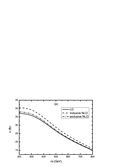
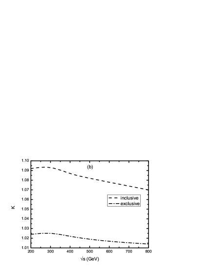
Figure 3: (a) The LO and ${\cal O}(\alpha_{s})$ QCD corrected cross sections with different event selection schemes for the $e^{+}e^{-}\to\gamma\gamma b\bar{b}$ as the functions of the colliding energy $\sqrt{s}$ at the ILC with $\mu=\sqrt{s}/2$, $p_{T,cut}^{(\gamma)}=10~{}GeV$, $p_{T,cut}^{(b)}=20~{}GeV$, $\Delta R_{\gamma\gamma}^{cut}=0.5$ and $\Delta R_{b\bar{b}}^{cut}=\Delta R_{b(\bar{b})\gamma}^{cut}=1$ for b-quarks and photons. (b) The corresponding K-factors versus $\sqrt{s}$.

$\sqrt{s}$(GeV)	200	300	400	500	800
$\sigma_{LO}(fb)$	37.19(1)	35.86(1)	31.86(1)	26.59(1)	14.947(8)
$\sigma_{QCD}(fb)$(I)	40.61(5)	39.20(5)	34.64(4)	28.77(3)	15.99(2)
$K$-$factor$(I)	1.092(3)	1.093(3)	1.087(3)	1.082(3)	1.070(3)
$\sigma_{QCD}(fb)$(II)	38.08(5)	36.77(5)	32.57(4)	27.10(3)	15.16(2)
$K$-$factor$(II)	1.024(3)	1.025(3)	1.021(3)	1.019(3)	1.014(3)

Table 1: The LO, ${\cal O}(\alpha_{s})$ QCD corrected cross sections and the corresponding K-factors with different jet veto schemes at the ILC by taking $\mu=\sqrt{s}/2$, $p_{T,cut}^{(\gamma)}=10~{}GeV$, $p_{T,cut}^{(b)}=20~{}GeV$, $\Delta R_{\gamma\gamma}^{cut}=0.5$ and $\Delta R_{b\bar{b}}^{cut}=\Delta R_{b(\bar{b})\gamma}^{cut}=1$. (I) For the ’inclusive’ three-jet event selection scheme. (II) For the ’exclusive’ three-jet event selection scheme.

Due to the CP-conservation, the $p_{T}^{(b)}$ distribution should be the same as anti-bottom’s ($p_{T}^{(\bar{b})}$). Here we present the LO and QCD corrected distributions of the transverse momenta for the bottom-quark and the leading photon with the ’inclusive’ three-jet event selection scheme in Fig.4(a) and Fig.4(b) respectively, the corresponding K-factors are also plotted there. The so-called leading photon is defined as the photon with the highest energy among the two final photons. These results are obtained by taking $\sqrt{s}=500~{}GeV$, $\mu=\sqrt{s}/2$ and the cut set for b-quarks and photons as mentioned above. From these two figures we can see that the ${\cal O}(\alpha_{s})$ QCD corrections enhance both the LO differential cross sections $d\sigma_{LO}/dp_{T}^{(b)}$ and $d\sigma_{LO}/dp_{T}^{(\gamma)}$, especially in low $p_{T}$ region. The $p_{T}^{(\gamma)}$ distribution curves in Fig.4(b) drop with growing $p_{T}^{(\gamma)}$. Fig.4(a) shows that the differential cross sections ($d\sigma_{LO}/dp_{T}^{(b)}$, $d\sigma_{NLO}/dp_{T}^{(b)}$) have their maximal values at about $30~{}GeV\sim 40~{}GeV$, but Fig.4(b) shows the maximal values of $d\sigma_{LO}/dp_{T}^{(\gamma)}$ and $d\sigma_{NLO}/dp_{T}^{(\gamma)}$ are located at about $p_{T}^{(\gamma)}=10~{}GeV\sim 20~{}GeV$.

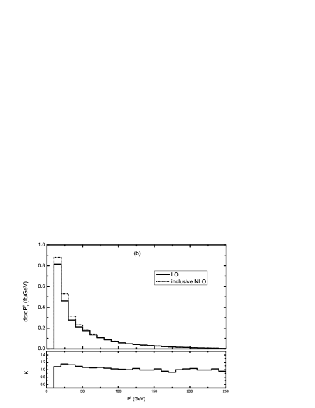
Figure 4: The LO and the ${\cal O}(\alpha_{s}\alpha^{4})$ distributions of the transverse momenta of bottom-quark and the leading photon, $p_{T}^{(b)}$, $p_{T}^{(\gamma)}$, in the conditions of $\sqrt{s}=500~{}GeV$, $\mu=\sqrt{s}/2$ and the ’inclusive’ selection scheme. There we take the cut values of $p_{T,cut}^{(\gamma)}=10~{}GeV$, $\Delta R_{\gamma\gamma}^{cut}=0.5$, $p_{T,cut}^{(b)}=20~{}GeV$ and $\Delta R_{b\bar{b}}^{cut}=\Delta R_{b(\bar{b})\gamma}^{cut}=1$. (a) The LO and ${\cal O}(\alpha_{s})$ QCD corrected distributions of transverse momentum of bottom-quark. (b) The LO and ${\cal O}(\alpha_{s})$ QCD corrected distributions of transverse momentum of the final leading photon.

We plot the spectra of $(b\bar{b})$- and $(\gamma\gamma)$-pair invariant masses (denoted as $M_{(b\bar{b})}$ and $M_{(\gamma\gamma)}$) with the ’inclusive’ three-jet event selection scheme at the LO and ${\cal O}(\alpha_{s}\alpha^{4})$ in Figs.5(a) and (b), respectively. There we take $\sqrt{s}=500~{}GeV$, $\mu=\sqrt{s}/2$, $p_{T,cut}^{(\gamma)}=10~{}GeV$, $\Delta R_{\gamma\gamma}^{cut}=0.5$, $p_{T,cut}^{(b)}=20~{}GeV$ and $\Delta R_{b\bar{b}}^{cut}=\Delta R_{b(\bar{b})\gamma}^{cut}=1$. We can see from Fig.5(a) that most of the events are concentrated around a peak located at the vicinity of $M_{(b\bar{b})}\sim m_{Z}$. That shows the fact that the contribution to the cross section for the $e^{+}e^{-}\to\gamma\gamma b\bar{b}$ process at the ILC, is mainly from real $Z^{0}$-boson production channel $e^{+}e^{-}\to\gamma\gamma Z^{0}$ and followed by the subsequent real $Z^{0}$ decay $Z^{0}\to b\bar{b}$. Both the Figs.5(a) and (b) show that the QCD corrections enhance the LO differential cross sections $d\sigma_{LO}/dM_{(b\bar{b})}$ and $d\sigma_{LO}/dM_{(\gamma\gamma)}$. The precise prediction for the distribution of the $(\gamma\gamma)$-pair invariant mass is very significant, because it is the irreducible continuum background for the Higgs-boson signature of $H^{0}\to\gamma\gamma$ decay in the $\gamma\gamma b\bar{b}$ production process.

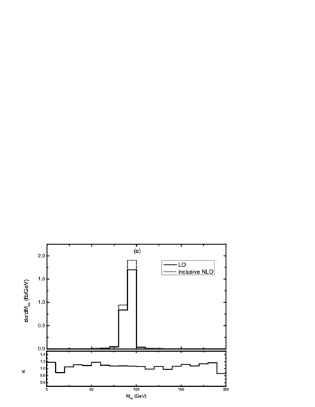
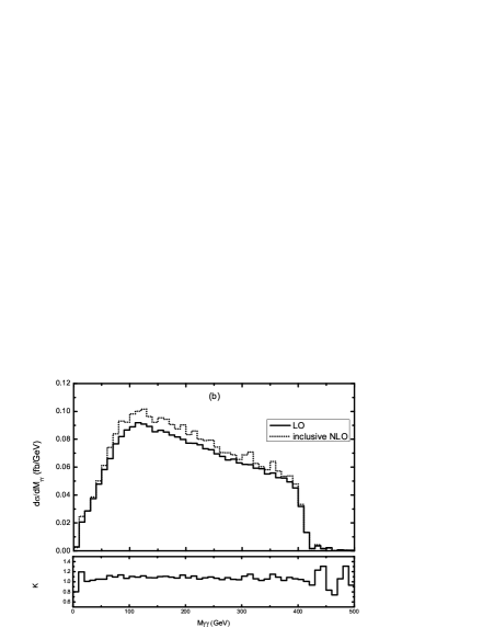
Figure 5: The distributions of the invariant masses of $(b\bar{b})$- and $(\gamma\gamma)$-pair at the LO and ${\cal O}(\alpha_{s}\alpha^{4})$ in conditions of $\sqrt{s}=500~{}GeV$, $\mu=\sqrt{s}/2$, $p_{T,cut}^{(\gamma)}=10~{}GeV$, $\Delta R_{\gamma\gamma}^{cut}=0.5$, $p_{T,cut}^{(b)}=20~{}GeV$ and $\Delta R_{b\bar{b}}^{cut}=\Delta R_{b(\bar{b})\gamma}^{cut}=1$. (a) The distribution of the invariant mass of $(b\bar{b})$-pair. (b) The distribution of the invariant mass of $(\gamma\gamma)$-pair.

IV. Summary

In this paper we calculate the complete ${\cal O}(\alpha_{s})$ QCD corrections to the $e^{+}e^{-}\to\gamma\gamma b\bar{b}$ process in the SM at the ILC. We study the dependence of the LO and ${\cal O}(\alpha_{s})$ QCD corrected cross sections on the colliding energy $\sqrt{s}$, and investigate the LO and ${\cal O}(\alpha_{s})$ QCD corrected distributions of the transverse momenta of final particles and the spectra of the invariant masses of $(\gamma\gamma)$- and $(b\bar{b})$-pair. The precise spectrum for the invariant mass of $\gamma\gamma$-pair is very important, since it is the irreducible background if the Higgs boson is produced via $e^{+}e^{-}\to H^{0}Z^{0}\to\gamma\gamma b\bar{b}$ channel. Our calculations show that the size of the ${\cal O}(\alpha_{s})$ QCD correction exhibits a obvious dependence on the additional gluon-jet veto scheme. The numerical results show that the QCD corrections with ’inclusive’ scheme enhance the LO results by about $9.2\%$ to $7.0\%$ when we take the cut of $p_{T,cut}^{(\gamma)}=10~{}GeV$, $\Delta R_{\gamma\gamma}^{cut}=0.5$, $p_{T,cut}^{(b)}=20~{}GeV$, $\Delta R_{b\bar{b}}^{cut}=\Delta R_{b(\bar{b})\gamma}^{cut}=1$ with the colliding energy running from $200~{}GeV$ to $800~{}GeV$.

Acknowledgments: This work was supported in part by the National Natural Science Foundation of China (Contract Nos.10875112, 10675110, 11005101, 11075150), and the Specialized Research Fund for the Doctoral Program of Higher Education (SRFDP)(No.20093402110030).

References

- [1] S.L. Glashow, Nucl. Phys, 22(1961)579; S. Weinberg, Phys. Rev. Lett. 1(1967)1264.
- [2] P.W. Higgs, Phys. Lett. 12(1964)132, Phys. Rev. Lett. 13(1964)508; Phys. Rev. 145, 1156 (1966); F. Englert and R. Brout, Phys. Rev. Lett. 13, 321 (1964); G. S. Guralnik, C. R. Hagen and T. W. B. Kibble, Phys. Rev. Lett. 13, (1964) 585; T. W. B. Kibble, Phys. Rev. Phys. Rev. 155, (1967) 1554.
- [3] G. Abbiendi.et al(the ALEPH, the DELPHI, the L3 and the OPAL, The LEP Working Group fot Higgs Boson Searches), Phys. Lett. B565 (2003) 61, arXiv:hep-ex/0306033.
- [4] The CDF, D0 Collaborations, the Tevatron New Phenomena, Higgs Working Group, “Combined CDF and D0 Upper Limits on Standard Model Higgs Boson Production with up to of Data”, FERMILAB-CONF-11-354-E, arXiv:1107.5518.
- [5] ATLAS Collaboration, “ATLAS experiment presents latest Higgs search status”, http://www.atlas.ch/news/2011/status-report-dec-2011.html
- [6] CMS Collaboration,“CMS search for the Standard Model Higgs Boson in LHC data from 2010 and 2011”, http://cms.web.cern.ch/news/cms-search-standard-model-higgs-boson-lhc-data-2010-and-2011.
- [7] E.Accomando et al., Phys. Rep. 299(1998)1, arXiv:hep-ph/9705442.
- [8] Abdelhak Djouadi, Joseph Lykken, Klaus Mönig, Yasuhiro Okada, Mark Oreglia, Satoru Yamashita, et al.,, arXiv:0709.1893, ILC Reference Design Report, http://www.linearcollider.org/about/Publications/Reference-Design-Report.
- [9] Proceeding of the Workshop on ’High Liminosities at LEP’, Geneva, Switzerland, 1991, CERN Report 91-02.
- [10] W. Kilian, M. Krämmer, P.M. Zerwas, Phys. Lett. B373(1996)135, ”Higgs Physics at Lep-2”, in CERN LEP-2 yellow report vol.1, CERN-96-01, arXiv:hep-ph/9602250; J. Fleischer and F. Jegerlehner, Nucl. Phys. B216 (1983) 469; B. A. Kniehl, Z. Phys. C55 (1992) 605; A. Denner, J. Kublbeck, R. Mertig, M. Böhm, Z. Phys. C56,(1992)261.
- [11] K. Nakamura, et al., J. Phys. G. 37 (2010) 075021.
- [12] J.-C. Brient, LC-PHSM-2002-003 (2002); K. Desch, arXiv:hep-ph/0311092.
- [13] E. Boos, J.-C. Brient, D.W. Reid, H.J. Schreiber, R. Shanidze, Eur. Phys. J. C19,(2001)455-461, arXiv:hep-ph/0011366.
- [14] Andre Sopczak, ’Higgs Physics: from LEP to a Future Linear Collider’, arXiv:hep-ph/0502002v1; Le Duc Ninh, ’One-Loop Yukawa Corrections to the Process in the Standard Model at the LHC: Landau Singularities’, LAPTH-1261/08, arXiv:0810.4078v2.
- [15] J.F. Gunion, P.C. Martin, Phys. Rev. Lett.78,4541(1997)arXiv:hep-ph/9607360.
- [16] S.D. Ellis, D.E. Soper, Phys. Rev. D48, 3160(1993), arXiv:hep-ph/9305266.
- [17] E. Boos, V. Bunichev, et al., (the CompHEP collaboration), Nucl. Instrum. Meth. A534 (2004) 250-259, arXiv:hep-ph/0403113.
- [18] T. Hahn, Comput. Phys. Commun. 140 (2001)418, arXiv:hep-ph/0012260.
- [19] A. Denner, S. Dittmaier, M. Roth, D. Wackeroth, Nucl. Phys. B560 (1999) 33, arXiv:hep-ph/9904472; A. Denner, S. Dittmaier, M. Roth, L.H. Wieders, Nucl. Phys. B724 (2005) 247, arXiv:hep-ph/0505042.
- [20] T. Hahn, M. Perez-Victoria, Comput. Phys. Commun. 118 (1999)153, arXiv:hep-ph/9807565.
- [21] S. Dittmaier, Nucl. Phys. B675(2003) 447, arXiv:hep-ph/0308246; W. Beenakker, S. Dittmaier et al., Nucl. Phys. B653(2003) 151, arXiv:hep-ph/0211352.
- [22] G.’t Hooft and M. Veltman, Nucl. Phys. B153 (1979) 365.
- [23] A. Denner, U Nierste and R Scharf, Nucl. Phys. B367 (1991) 637.
- [24] A. Denner and S. Dittmaier, Nucl. Phys. B658 (2003) 175, arXiv:hep-ph/0212259.
- [25] G. Passarino and M. J. G. Veltman, Phys. Lett. B237,(1990)537.
- [26] M. Chanowitz, M. Furman, and I. Hinchliffe, Nucl. Phys. B159 (1979) 225.
- [27] B. W. Harris and J.F. Owens, Phys. Rev. D65 (2002) 094032, arXiv:hep-ph/0102128.
- [28] S. Catani and M.H. Seymour, Phys. Lett. B378 (1996) 287, arXiv:hep-ph/0102128; Nucl. Phys. B485 (1997) 291, arXiv:hep-ph/9605323. Erratum, ibid. B510 (1998) 503; Stefan Dittmaier, Nucl. Phys. B565 (2000)69, arXiv:hep-ph/9904440.