A Class Coupler for Perfect Sampling from Continuous Distributions With and Without Atoms

Abstract

We consider the simulation of distributions that are a mixture of discrete and continuous components. We extend a Metropolis-Hastings-based perfect sampling algorithm of Corcoran and Tweedie [5] to allow for a broader class of transition candidate densities. The resulting algorithm, know as a “class coupler”, is fast to implement and is applicable to purely discrete or purely continuous densities as well. Our work is motivated by the study of a composite hypothesis test in a Bayesian setting via posterior simulation and we give simulation results for some problems in this area.

1 Introduction

It has been more than a decade since the appearance of the seminal paper of Propp and Wilson [19] which introduced perfect simulation to the Monte Carlo community. Immediately thereafter, several variations and extensions [6, 7, 8, 11, 13, 17, 18] appeared, proving to be effective in areas such as statistical physics, spatial point processes and operations research, where they provided simple and powerful alternatives to existing methods based on, for example, iterating transition laws.

In this paper, we extend a perfect sampling algorithm of Corcoran and Tweedie [5] so that it is applicable to a larger class of probability models. In particular, our algorithm is useful for simulating densities that are a mixture of continuous and discrete densities. Our approach was motivated by the study of a composite hypothesis test in a Bayesian setting such as

$$H_{0}:\theta=\theta_{0}$$

versus

$$H_{1}:\theta\neq\theta_{0},$$

where $\theta$ is a model parameter with a “mixed” distribution that takes on values in a continuum but allows for the possibility that $\theta=\theta_{0}$. Thus, it becomes necessary to impose a mixed prior density on $\theta$ which results in a mixed posterior density as well.

In order to simulate values from the mixed posterior density we have adapted a perfect version of the Metropolis-Hastings algorithm in [5] where we somewhat relax an assumption that a Markov chain candidate transition density proposes future states independent of current states. We refer to our algorithm as a “class coupler” as it relies on a partitioning of the state space into subspaces or classes. In the context of the above described mixture target density the atom at $\theta_{0}$ is designated as one (single point) class while the remaining possibilities for $\theta$ comprise the members of a second class. In general though, we may decompose the state space of the target density into several classes and it is not necessary that there be any atoms.

In Section 2, we give a brief review of the concept of perfect sampling, the Metropolis-Hastings algorithm, and of the existing perfect version of the Metropolis-Hastings algorithm of Corcoran and Tweedie [5]. In Section 3, we describe our extension which is known as the class coupler. In Section 4, we provide some simulation examples for Bayesian regression models and compare our results to those of Gottardo and Raftery [9].

2 Perfect Sampling

A Markov chain Monte Carlo (MCMC) algorithm that would enable one to draw values from a given density $\pi(\cdot)$ such as is a recipe for creating a Markov chain $\{X_{n}\}$ so that

$$\lim_{n\rightarrow\infty}P(X_{n}\in A)=\pi(A).$$ (1)

Here, $A$ is a subset of the state space of $\{X_{n}\}$ and $\pi(A)$ is shorthand notation for $\int_{A}\pi(x)\,dx$.

Quantities involving $\pi(\cdot)$ are then usually approximated by simulating values of $X_{N}$ for some very large $N$. The advantage of perfect sampling (also known as perfect simulation) over this traditional MCMC approach allows us to directly sample (simulate) values of $X_{\infty}$.

The essential idea behind perfect sampling is to find a random epoch $-T$ in the past such that, if we construct sample paths (according to a transition law $P(x,A):=P(X_{n+1}\in A|X_{n}=x)$ that is converging to $\pi$) from every point in the state space starting at $-T$, then all paths will come together and meet or “couple” by time zero. The common value of the paths at time zero is a draw from $\pi$. Intuitively, it is clear why this result holds with such a random time $T$ as we are constructing the tail end of a path that has traveled forward from time $-\infty$ since any such path will pass through the time point $-T$ and then be “funneled forward” to the common value at time zero. We refer to the smallest value of $T$ for which this can be achieved as a backward coupling time (BCT).

For more details on perfect sampling, we refer the interested reader to Casella, Lavine, and Robert [3].

2.1 The (Non-Perfect) Metropolis-Hastings Algorithm

Suppose we wish to simulate values from a target distribution with density $\pi(x)$ for $x\in{\rm I\!R}^{k}$. The Metropolis-Hastings algorithm [24] is one way to construct a Markov chain and transition probabilities with our target distribution as its limiting distribution.

In order to describe the Metropolis-Hastings algorithm(s), we consider a candidate transition kernel $Q(x,A)$ for $x\in{\rm I\!R}^{k}$ and a Borel set $A\subset{\rm I\!R}^{k}$ satisfying

$$Q(x,A)\geq 0\qquad\mbox{and}\qquad Q(x,{\rm I\!R}^{k})=1$$

which generates potential transitions for a discrete-time Markov chain evolving on ${\rm I\!R}^{k}$. We assume that there exists a density $q(x,y)$ such that

$$Q(x,A)=\int_{A}q(x,y)\,dy.$$

The Metropolis algorithm [15], dating back to 1953, uses a symmetric candidate transition $Q$ for which $q(x,y)=q(y,x)$. In 1970, Hastings [23] extended the Metropolis algorithm to a more general $Q$. In either case, the simulator proceeds by generating candidate transitions from state $x$ to state $y$ according to the distribution $Q$, and accepting the transition with probability

$$\alpha(x,y)=\left\{\begin{array}[]{ll}\min\left\{1,\,\,{\displaystyle\frac{\pi(y)}{\pi(x)}\frac{q(x,y)}{q(y,x)}}\right\}&\pi(x)q(y,x)>0\\ 1&\pi(x)q(y,x)=0.\end{array}\right.$$ (2)

Thus evolves a Markov chain with transition density

$$p(x,y)=q(x,y)\,\alpha(x,y),\qquad y\neq x,$$

which will remain at the same point with probability

$$P(x,\{x\})=\int q(x,y)\,[1-\alpha(x,y)]\,dy.$$

It is easy to verify that $\pi$ is the invariant or stationary measure for the chain in the sense that

$$\pi(A)=\int\pi(x)P(x,A)\,dx,\qquad\forall A\in{\cal{B}}({\sf X})$$

where ${\sf X}$ is the state space of the chain and ${\cal{B}}({\sf X})$ are the Borel sets in ${\sf X}$.

It is also easy to verify that any limiting distribution is stationary and that, for this chain constructed with the Metropolis-Hastings algorithm, there is a unique stationary distribution. Thus, the stationary and limiting distributions are one and the same.

Note that due to its presence only in ratios, we can run this algorithm even if we only know $\pi$ up to a constant of proportionality.

In order to simulate a value drawn from $\pi$, one must generally select a distribution $Q$ and run a Metropolis-Hasting sample path for “a long time” until it is suspected that convergence to $\pi$ has been achieved. Choices for $Q$ and rates of convergence have been studied extensively in [2],[14], and [22], for example.

2.2 The Perfect Independent Metropolis-Hastings Algorithm

In Corcoran and Tweedie [5], a Metropolis-Hastings-based perfect sampling algorithm was introduced, eliminating the need to address issues of convergence.

We use the term “independent” to describe the Metropolis-Hastings algorithm where candidate states are generated by a distribution $Q$ that is independent of the current state of the chain. In this Section, we assume the existence of a density $q(x,y)$ such that

$$Q(x,A)=\int_{A}q(x,y)\,dy.$$

Assuming an independent candidate density means that

$$q(x,y)\equiv q(y).$$

The perfect independent Metropolis-Hastings (perfect IMH) algorithm uses the ratios in the acceptance probabilities given by (2) to reorder the states in such a way that we always accept moves to the left (or downwards). That is, if we write $\pi(x)=kh(x)$ where $k$ is possibly unknown, we define the IMH ordering,

$$x\succeq y\qquad\Longleftrightarrow\qquad\frac{\pi(y)q(x)}{\pi(x)q(y)}\geq 1\qquad\Longleftrightarrow\qquad\frac{h(y)}{q(y)}\geq\frac{h(x)}{q(x)}$$ (3)

With this ordering, we can (hopefully) attain a “lowest state” $\ell$ for which $h(l)/q(l)\geq h(x)/q(x)$ for all $x$ in the state space. Given the role of $h/q$ in the acceptance probability of the Metropolis-Hasting algorithm, one can think of $\ell$ as the state that is hardest to move away from when running the IMH algorithm. Thus, if we are able to accept a move from $\ell$ to a candidate state $y$ drawn from the distribution $Q$ with density $q$, then sample paths from every point in the state space will also accept a move to $y$, so all possible sample paths will couple. For the following formal description of the steps of the algorithm, we will assume the existence of a “highest” point $u$ for which $h(u)/q(u)\leq h(x)/q(x)$ for all $x$. The existence of such a point is not required though as will be noted directly after the algorithm description.

Perfect IMH Algorithm

1. Draw a sequence of random variables $Q_{-n}\sim Q$ for $n=0,1,2,\ldots$, and a sequence $\alpha_{-n}\sim\mbox{Uniform}(0,1)$ for $n=1,2,\ldots$.

2. For each time $-n=-1,-2,\ldots$, start a lower path $L$ at $\ell$, and an upper path, $U$ at $u$.

3. 1. For the lower path: Accept a move from $\ell$ to $Q_{-n+1}$ at time $-n+1$ with probability $\alpha(l,Q_{-n+1})$, otherwise remain at state $\ell$. That is, accept the move from $\ell$ to $Q_{-n+1}$ if $\alpha_{-n}\leq\alpha(l,Q_{-n+1})$.

   2. For the upper path: Similarly, accept a move from $u$ to $Q_{-n+1}$ at time $-n+1$ if $\alpha_{-n}\leq\alpha(u,Q_{-n+1})$; otherwise remain at state $Q_{-n}$.

4. Continue until $T$ defined as the first $n$ such that at time $-n+1$ each of these two paths accepts the point $Q_{-n+1}$. (Continue the Metropolis-Hastings algorithm forward to time zero using the same sequence of $\alpha$’s and $Q$’s produced in steps 1-3 to get the draw from $\pi$ at time zero.)

There is a monotonicity imposed by (3) such that for any candidate point $y$,

$$x_{1}\succeq x_{2}\qquad\Rightarrow\qquad\alpha(x_{1},y)<\alpha(x_{2},y).$$

Consequently, if any point accepts a move to $y$, all “higher” points will also accept a move to this candidate. Therefore, the upper path in this algorithm will accept a candidate point whenever the lower path will, and the two paths will be the same from that time forward. Consequently, our description of the upper process is a formality only, and, indeed, the upper process need not be run at all. Therefore, the point $u$ does not need to be identified and in fact is not even required to exist!

Figure 1 illustrates a realization of the perfect IMH algorithm.

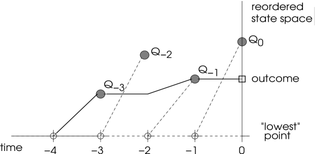
Figure 1: A Realization of the Perfect IMH Algorithm With Backward Coupling Time at -4

Dashed grey lines represent potential but unrealized arcs of the sample path. Solid grey lines represent the sample paths started at times -1, -2, and -3 that did not achieve the coupling. The solid black line represents the path whose outcome is ultimately observed in the perfect sampling algorithm.

3 Our Extension: “The Class Coupler”

We now extend the perfect IMH algorithm to allow for a transition candidate density that can depend on the current state of the chain up to the inclusion of that state in a set found in a partition of the state space. Specifically, we will partition the state space into sets or “classes” ${\cal{C}}_{1},{\cal{C}}_{2},\ldots,{\cal{C}}_{K}$ and allow for a transition candidate density of the form

$$q(x,y)=q_{{\cal{C}}_{i}}(y)\qquad\mbox{for}\,\,\,x\in{\cal{C}}_{i}$$

for some independent transition candidate density $q_{{\cal{C}}_{i}}(\cdot)$.

We begin with a simple two class partition.

3.1 A Continuous Distribution With a Single Atom

Suppose that we have a sample $\vec{X}=(X_{1},X_{2},\ldots,X_{m})$ from a density $f(\vec{x}|\theta)$ with a prior density $f_{\theta}(\cdot)$ of the form

$$f_{\theta}(\cdot)=p\cdot\delta_{0}(\cdot)+(1-p)f_{1}(\cdot),$$ (4)

where $f_{1}(\cdot)$ is a continuous density, $0<p<1$, and $\delta_{0}(\cdot)$ is the Dirac delta function with point mass concentrated at zero. $f_{1}$ may depend on known hyperparameters.

Further suppose that we wish to test

$$H_{0}:\theta=0\qquad\mbox{versus}\qquad H_{1}:\theta\neq 0.$$

by drawing values from the posterior distribution with density

$$\pi(\theta)\equiv\pi(\theta|\vec{x})\propto f(\vec{x}|\theta)\cdot f_{\theta}(\theta).$$ (5)

(The null value $0$ is used here only for simplicity and may be replaced with a generic $\theta_{0}$.)

In this paper, we are concerned only with the Monte Carlo algorithm that will allow us to obtain perfect draws from $\pi(\theta)$ and not with what one should do with such values in order to make a decision about the given hypotheses. Typically, one would report and interpret posterior odds ratio or a Bayes factor. We refer the reader to [20] for details about Bayesian hypothesis testing in general.

In order to simulate the density in (5), we will use a Metropolis-Hastings algorithm with transition candidate density

$$q(\theta,\theta^{\prime})=\left\{\begin{array}[]{lcl}\delta_{0}(\theta^{\prime})&,&\mbox{if}\,\,\,\theta\neq 0\\ \\ g(\theta^{\prime})&,&\mbox{if}\,\,\,\theta=0\\ \end{array}\right.$$ (6)

where $g(\cdot)$ is some continuous density that will be chosen in a convenient way. Note that this candidate density is no longer an independent candidate density. That is, the right-hand side of (6) is not independent of $\theta$.

For the regular forward (non-perfect) Metropolis-Hastings algorithm, one would proceed to draw approximate values from $\pi(\theta)$ as follows.

1. Start with some (perhaps arbitrary) value of $\theta$.

2. Propose another value $\theta^{\prime}$ by drawing a value from the distribution with density $q(\theta,\cdot)$.

3. With probability

   $$\alpha(\theta,\theta^{\prime})=\min\{1,r(\theta,\theta^{\prime})\}$$

   where

   $$r(\theta,\theta^{\prime})=\frac{\pi(\theta^{\prime})q(\theta^{\prime},\theta)}{\pi(\theta)q(\theta,\theta^{\prime})}=\frac{f(\vec{x}|\theta^{\prime})f_{\theta}(\theta^{\prime})q(\theta^{\prime},\theta)}{f(\vec{x}|\theta)f_{\theta}(\theta)q(\theta,\theta^{\prime})}.$$

   accept the move to $\theta^{\prime}$ and set $\theta=\theta^{\prime}$.

4. Return to Step 2.

After “many” iterations of Steps 2 through 4, one could output the current value of the chain as an approximate draw from $\pi(\theta)$. We would arrive at a perfect draw from $\pi(\theta)$ after an infinite number of iterations.

In order to turn this into a perfect simulation algorithm, we need to run through backward time steps (taking care to reuse the random variates associated with each time step) and we need to be able to figure out if and when all possible paths wandering through the state space of $\theta$ will meet. Consider Figure 2 which depicts the possible updates of sample paths of the MH-chain between time steps $-4$ and $-3$. At time $-4$ the point $\theta=0$ is depicted as well as an arbitrary non-zero value for $\theta$.

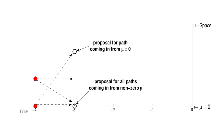
Figure 2: Possible Updates of Sample Paths of the MH-Chain with Candidate Transitions Generated by $q(\theta,\theta^{\prime})$ from (6)

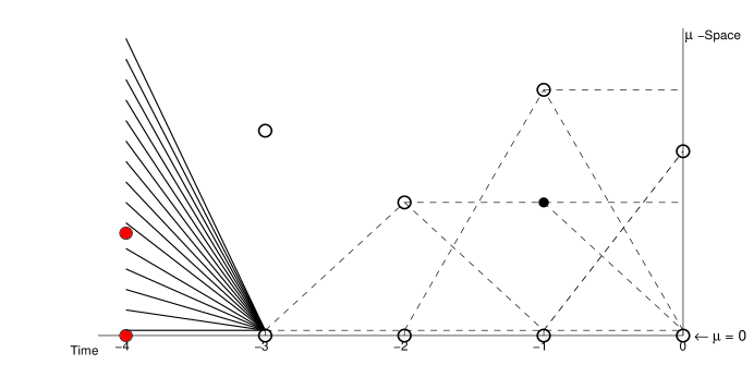
Figure 3: One Case of Coupling

All sample paths have coupled at time $-3$. From there, dashed lines represent potential paths forward to time zero following a series of possible acceptance or rejections of candidate points which are depicted as open circles. For this particular image, the perfect draw from $\pi$ will be one of 4 points indicated at time zero, depending on which dashed lines are followed.

One way to achieve a coupling of all sample paths is in the case that all sample paths starting at $\theta\neq 0$ accept the proposed value of $0$ and the path starting at $\theta=0$ rejects its proposed non-zero value and stays at zero. This is depicted in Figure 3.

Another way to achieve coupling is in the case that all sample paths starting at $\theta\neq 0$ accept the proposed value of $0$ and the path starting at $\theta=0$ accepts its proposed non-zero value, but at a later time (before time $0$) the resulting two paths manage to meet. This is depicted in Figure 4. (It is important to note that this realization only becomes relevant after failed attempts at achieving full coupling starting first at time $-1$, then at time $-2$, and then at time $-3$.)

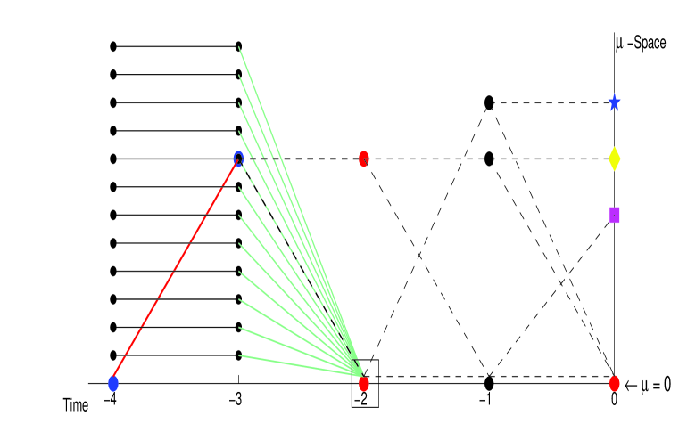
Figure 4: A Second Case of Coupling With a Backward Coupling Time of $-4$

Open circles in this Figure represent candidate values for possible transitions. Dashed lines represent potential transitions while solid lines represent actual realized transitions.

From time $-4$ to time $-3$: All sample paths from non-zero $\theta$ have accepted the candidate value of $0$ at time $-3$. The sample path from state $0$ has accepted the non-zero candidate value.

From time $-3$ to time $-2$: The path that is non-zero at time $-3$ fails to accept the $0$ candidate value at time $-2$ and “stays flat”. That path that is at $0$ at time $-3$ accepts the proposed non-zero candidate at time $-2$.

From time $-2$ to time $-1$: We are now following two non-zero paths. In this depiction, both have accepted the $0$ candidate and coupling is achieved at time $-1$. Continuing this single path forward to time $0$ results in a perfect draw from the desired distribution which is shown in a box. Assuming previously failed attempts starting from all points at times

$-1$, $-2$, and $-3$, we say that the backward coupling time is $-4$.

To determine when all non-zero paths accept a zero candidate, we must find

$$\min_{\theta\neq 0}\,r(\theta,0).$$ (7)

This is the smallest probability of acceptance of zero for all non-zero paths. In a simulation, we would have random numbers, $\alpha_{-1},\alpha_{-2},\ldots$, uniformly distributed on $[0,1]$, associated with each negative time step. All non-zero paths at time $-t$ will accept a move to the proposal zero at time $-t+1$ if

$$\alpha_{-t}\leq\min_{\theta\neq 0}r(\theta,0).$$

As we are free to choose the density $g(\cdot)$ in (6), we choose it to be the same as $f_{1}(\cdot)$, which is the density used in the mixture prior (4). This results in a simplification of $r(\theta,\theta^{\prime})$.

Since

$$r(\theta,0)=\frac{p}{1-p}\cdot\frac{f(\vec{x}|0)}{f(\vec{x}|\theta)},$$ (8)

$r(\theta,0)$ is clearly minimized at the maximum likelihood estimator (MLE) of $\theta$, which we will denote by $\hat{\theta}$.

3.1.1 Complete Algorithm Details

We include this Section in order to clarify the details of the class coupler especially as it pertains to reusing random deviates from earlier time steps. It serves as a reference that may be useful in algorithm implementation but can be skipped in a reading of this paper

Algorithm:

Let $t=1$. Compute

$$r(\hat{\theta},0)=\frac{p}{1-p}\cdot\frac{f(\vec{x}|0)}{f(\vec{x}|\hat{\theta})}.$$

1. Generate random deviates $Q_{-t+1}\sim f_{1}$ and $\alpha_{-t}\sim\mathrm{Uniform}(0,1).$
   Compute

   $$r(0,Q_{-t+1})=\frac{1-p}{p}\cdot\frac{f(\vec{x}|Q_{-t+1})}{f(\vec{x}|0)}.$$

2. If

   • $r(\hat{\theta},0)<\alpha_{-t}\leq r(0,Q_{-t+1})$, we have achieved the one-step coupling depicted in Figure 3. Set $X_{-t+1}=0$. Record the backward coupling time as $T=t$. Go to Step $4$.

   • $\alpha_{-t}\leq\min(r(\hat{\theta},0),r(0,Q_{-t+1}))$, we have achieved the first stage of the coupling depicted in Figure 4. Set $X_{-t+1}^{(1)}=Q_{-t+1}$ and $Q_{-t+1}^{(2)}=0$. If $t>1$, go to Step $3$ to attempt the second stage of coupling. If $t=1$, return to Step 1.

   Otherwise, set $t=t+1$ and return to Step 1.

3. Second stage for two stage coupling: Run the usual forward MH simulations, using existing random deviates $Q_{-t+2},Q_{-t+3}\ldots,Q_{0}$ and $\alpha_{-t+1},\alpha_{-t+2}\ldots,\alpha_{1}$ until both paths, started at $X_{-t+1}^{(1)}$ and $X_{-t+1}^{(2)}$ reach time zero.

   For $i=1,2$, this is accomplished by setting, for $k=t-2,t-3,\ldots,0$,

   $$X_{-k}^{(i)}=\left\{\begin{array}[]{lcl}Q_{-k}&,&\mbox{if}\,\,\,\alpha_{-k-1}\leq r(X_{-k-1}^{(i)},Q_{-k})\\ \\ X_{-k-1}^{(i)}&,&\mbox{otherwise}\end{array}\right.$$

   • If $X_{0}^{(1)}=X_{0}^{(2)}$, stop. $X_{0}^{(1)}$ is a perfect draw from target distribution and the backward coupling time is $T=t$.

   • If $X_{0}^{(1)}\neq X_{0}^{(2)}$, set $t=t+1$ and return to Step 1.

4. Run the single path, starting from $X_{-t+1}=0$, forward using the existing random deviates $Q_{-t+2},Q_{-t+3}\ldots,Q_{0}$ and $\alpha_{-t+2},\alpha_{-t+3}\ldots,\alpha_{1}$ by, for $k=t-2,t-3,\ldots,0$, setting

   $$X_{-k}=\left\{\begin{array}[]{lcl}Q_{-k}&,&\mbox{if}\,\,\,\alpha_{-k-1}\leq r(X_{-k-1},Q_{-k})\\ \\ X_{-k-1}&,&\mbox{otherwise}\end{array}\right.$$

   Stop. The value reached at time zero, $X_{0}$, is a perfect draw from the target distribution.

3.2 A More General Algorithm

We extend the perfect algorithm used in Section 3.1 to a more general situation. There, we partitioned the state space for $\theta$ into the point $0$ and the class of non-zero points. In general, we can to partition the state space into two or more non-overlapping classes. In the case of $K$ classes, we modify the algorithm described in Section 3.1 by using a single candidate value for all points in class $i$ from a density, $q_{i}(\cdot)$. For simplicity, especially as it pertains to computing acceptance probabilities, it is advisable to not include class $i$ points in the support of $q_{i}(\cdot)$. For example, in the case of two classes, labeled I and II, we recommend proposing single candidate value for all class I points from a density, $q_{I}(\cdot)$, with support in class II and proposing a single candidate value for all class II points from a density, $q_{II}(\cdot)$ with support in class I. Allowing “within-class” proposals may lower the backward coupling times but will complicate the minimization of acceptance probabilities.

Each time an entire class of points accepts a transition candidate point, the cardinality of the number of sample paths to be followed is reduced. The goal, of course, is to reduce to a single path before time $0$.

4 Examples

4.1 A Simple Bayesian Regression Model

Consider the model

$$Y_{j}=\mu+\epsilon_{j},\qquad j=1,2,\ldots,n$$ (9)

where the $\epsilon_{j}$ are independent and identically distributed as

$$\epsilon_{j}|\sigma^{2}\sim N(0,v).$$

We assume a normal prior on $\mu$ with an atom at $0$:

$$f(\mu|p,\sigma_{\mu}^{2})=p\cdot\delta_{0}(\cdot)+(1-p)\cdot N(\mu;0,\sigma_{\mu}^{2})$$

with known hyperparameters $p$ and $\sigma_{\mu}^{2}$. Here, $N(\cdot;0,\sigma_{\mu}^{2})$ is the normal density with mean $0$ and variance $\sigma_{\mu}^{2}$.

We assume that we do not know the variance parameter for $\epsilon_{j}$ but we impose an inverse gamma prior with known hyperparameters $k_{1}$ and $k_{2}$. (This means that $1/v$ has a gamma distribution with mean $k_{1}/k_{2}$ and variance $k_{1}/k_{2}^{2}$.) We will assume that, a priori, $\mu$ and $v$ are independent, so that the posterior (target) density has the form

$$\pi(\mu,v)\equiv\pi(\mu,v|\vec{y})\propto f(\vec{y}|\mu,v)\cdot f(\mu|p,\sigma_{\mu}^{2})\cdot IG(v;k_{1},k_{2})$$

where $IG(\cdot;k_{1},k_{2})$ is the inverse gamma density.

We will simulate values from $\pi(\mu,v)$ using the class coupler with

$$\mbox{class I}=\{(0,v):v>0\}$$

and

$$\mbox{class II}=\{(\mu,v):-\infty<\mu<\infty,\mu\neq 0,v>0\}.$$

Consider the candidate transition density

$$q((\mu,v),(\mu^{\prime},v^{\prime}))=q_{1}(\mu,\mu^{\prime})\cdot q_{2}(v,v^{\prime})$$

where

$$q_{1}(\mu,\mu^{\prime})=\left\{\begin{array}[]{lcl}\delta_{0}(\mu^{\prime})&,&\mbox{if}\,\,\,\mu\neq 0\\ \\ g(\mu^{\prime})=N(\mu^{\prime};0,\sigma_{\mu}^{2})&,&\mbox{if}\,\,\,\mu=0\\ \end{array}\right.$$

and

$$q_{2}(v,v^{\prime})=q_{2}(v^{\prime})=IG(v^{\prime};k_{1},k_{2}).$$

Clearly, class II points will always have a proposed transition in class I. In order to determine that all points accept this proposal, we need to minimize

$$\begin{array}[]{lcl}r((\mu,v),(0,v^{\prime}))&=&{\displaystyle\frac{f(\vec{y}|0,v^{\prime})\cdot f(0|p,\sigma_{\mu}^{2})\cdot q((0,v^{\prime}),(\mu,v))}{f(\vec{y}|\mu,v)\cdot f(\mu|p,\sigma_{\mu}^{2})\cdot q((\mu,v),(0,v^{\prime}))}}\\ \\[7.22743pt] &=&{\displaystyle\frac{p}{1-p}\cdot\frac{f(\vec{y}|0,v^{\prime})}{f(\vec{y}|\mu,v)}}\end{array}$$

over class II points. The minimum occurs at the MLEs $\hat{\mu}$ and $\hat{v})$ where

$$\hat{\mu}=\overline{Y}=\frac{1}{n}\sum_{i=1}^{n}Y_{i}\qquad\mbox{and}\qquad\hat{v}=\frac{1}{n}\sum_{i=1}^{n}(Y_{i}-\overline{Y})^{2}.$$

Similarly, class I points will always have a proposed transition in class II. In order to determine that all points accept this proposal, we need to minimize

$$\begin{array}[]{lcl}r((0,v),(\mu^{\prime},v^{\prime}))&=&\frac{\displaystyle f(\vec{y}|\mu^{\prime},v^{\prime})\cdot f(\mu^{\prime}|p,\sigma_{\mu}^{2})\cdot q((\mu^{\prime},v^{\prime}),(0,v))}{\displaystyle f(\vec{y}|0,v)\cdot f(0|p,\sigma_{\mu}^{2})\cdot q((0,v),(\mu^{\prime},v^{\prime}))}\\ \\ &=&\frac{\displaystyle 1-p}{\displaystyle p}\cdot\frac{\displaystyle f(\vec{y}|\mu^{\prime},v^{\prime})}{\displaystyle f(\vec{y}|0,v)}\end{array}$$

over class I points. The minimum occurs at the restricted MLE

$$\hat{v}_{0}=\frac{1}{n}\sum_{i=1}^{n}Y_{i}^{2}.$$

Algorithm:

Let $t=3$. (A full coupling of sample paths will take at least three steps due to the multi-stage nature of the coupler.) Generate and store independent random deviates $S_{0}$, $S_{-1}$, $N_{0}$, $N_{-1}$, and $U_{-1}$, $U_{-2}$, where $S_{i}\sim IG(k_{1},k_{2})$, $N_{i}\sim N(0,\sigma_{\mu}^{2})$, and $U_{i}\sim\mbox{Uniform}(0,1)$.

1. Generate and store $S_{-t+1}\sim IG(k_{1},k_{2})$, $N_{-t+1}\sim N(0,\sigma_{\mu}^{2})$, and $U_{-t}\sim\mbox{Uniform}(0,1)$.

   Compute

   $$r((\hat{\mu},\hat{v}),(0,S_{-t+1}))=\frac{p}{1-p}\cdot\frac{f(\vec{y}|0,S_{-t+1})}{f(\vec{y}|\hat{\mu},\hat{v})}$$

   and

   $$r((0,\hat{v}_{0}),(N_{-t+1},S_{-t+1}))=\frac{1-p}{p}\cdot\frac{f(\vec{y}|N_{-t+1},S_{-t+1})}{f(\vec{y}|0,\hat{v}_{0})}$$

2. If

   • $U_{-t}\leq\min(r((\hat{\mu},\hat{v}),(0,S_{-t+1})),r((0,\hat{v}_{0}),(N_{-t+1},S_{-t+1})))$, we have achieved the first stage of the desired coupling. Set $X_{-t+1}^{(1)}=(0,S_{-t+1})$ and $X_{-t+1}^{(2)}=(N_{-t+1},S_{-t+1})$. Set $T=t$.

   • $U_{-t}>\min(r((\hat{\mu},\hat{v},(0,S_{-t+1})),r((0,\hat{v}_{0}),(N_{-t+1},S_{-t+1})))$, set $t=t+1$ and return to Step 1.

3. Run forward to time zero as follows.

   Let $k=-t+1$, and let $X_{k}^{(i)}(j)$ denote the $j$th component of $X_{k}^{(i)}$ for $j=1,2$.

   1. For $i=1,2$,

      • If $X_{k}^{(i)}(1)=0$, compute

        $$r((X_{k}^{(i)}(1),X_{k}^{(i)}(2)),(N_{k+1},S_{k+1}))=\frac{p}{1-p}\cdot\frac{f(\vec{y}|N_{k+1},S_{k+1})}{f(\vec{y}|(X_{k}^{(i)}(1),X_{k}^{(i)}(2)))}.$$

        If $U_{k}\leq r((X_{k}^{(i)}(1),X_{k}^{(i)}(2)),(N_{k+1},S_{k+1}))$, set $X_{k+1}^{(i)}=(N_{m+1},S_{k+1})$.

        Otherwise, set $X_{k+1}^{(i)}=X_{k}^{(i)}$.

      • If $X_{k}^{(i)}(1)\neq 0$, compute

        $$r(((X_{k}^{(i)}(1),X_{k}^{(i)}(2)),(0,S_{k+1}))=\frac{1-p}{p}\cdot\frac{f(\vec{y}|0,S_{k+1})}{f(\vec{y}|(X_{k}^{(i)}(1),X_{k}^{(i)}(2)))}.$$

        If $U_{k}\leq r(((X_{k}^{(i)}(1),X_{k}^{(i)}(2)),(0,S_{k+1}))$, set $X_{k+1}^{(i)}=(0,S_{k+1})$.

        Otherwise, set $X_{k+1}^{(i)}=X_{k}^{(i)}$.

   2. Set $k=k+1$.

      • If $k<0$, return to Step 3a.

      • If $k=0$ and $X_{0}^{(1)}\neq X_{0}^{(2)}$, set $t=t+1$ and return to Step 1.

      • If $k=0$ and $X_{0}^{(1)}=X_{0}^{(2)}$, Stop. $X_{0}^{(1)}$ is a perfect draw from $\pi(\mu,v)$ and the backward coupling time is $T$.

It is important to note that in the first bullet point of Step 2 of the above algorithm, we have required that all class I points accept a candidate and all class II points accept a class I candidate in the same time step. This is depicted in Figure 5. This is a conservative algorithm in the sense that it will give a longer backward coupling time than allowing class acceptances in different time steps, however it is much simpler to execute. Allowing both classes to accept in different time steps will require us to potentially follow many more paths, the number of which will be variable and generally increasing in time.

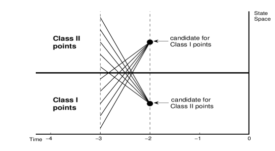
Figure 5: A Two class Coupler

Coupling may occur in this two class case when all paths from class I accept their candidate value which is proposed in class II and all paths from class II accept their candidate value which is proposed in class I. After this, we need to follow only two sample paths forward to time zero. Coupling occurs if these two paths meet before time zero.

Results: Simulation One

For this simulation, we used data and hyperparameters identical to those used in a standard non-perfect Monte Carlo simulation in Gottardo and Raftery [9]. They provided $10$ randomly generated observations from a $N(0.5,1)$ distribution as:

$$0.575,\,\,\,1.808,\,\,\,0.532,\,\,\,-0.168,\,\,\,0.529,\,\,\,0.888,\,\,\,-1.368,\,\,\,-0.512,\,\,\,2.667,\,\,\,0.874.$$

Hyperparameters were $p=0.5$, $\sigma_{\mu}^{2}=100$, $k_{1}=1$, and $k_{2}=0.05$.

The resulting values of $\mu$ marginalized from a perfect class coupler simulation of $\pi(\mu,v)$ are shown in Figure (6a). The estimated posterior probability that $\mu=0$, based on $100,000$ independent draws, $0.86907$ which gives an approximate 95% confidence interval for this posterior probability as $(0.86694,0.87120)$.

This gives positive, but not what is conventionally viewed as strong evidence ([9], [12]), for the null hypothesis, $H_{0}:\mu=0$.

For comparison, the Gottardo and Raftery [9] paper gives three different estimates and standard deviations for the posterior probability that $\mu=0$. They are

$$0.858\,(0.0054),\,\,\,0.870\,(0.0031),\,\,\,\mbox{and}\,\,\,0.865\,(0.0036).$$

The first and second estimates are from forward Metropolis-Hastings algorithms with different candidate distributions. The third estimate is from a Gibbs sampler. All are based on $10,000$ dependent draws from a single Markov chain collected after a burn-in period of $1,000$ time steps. Although they are close to our estimate, the length of the burn in period seems to have been arbitrarily chosen and convergence is not assured. For our results, we have chosen to produce independent draws for $\mu$ as allowed by the speed of the class coupler. The mean backward coupling time in our $100,000$ draws was $1502.6$ with a minimum of $6$ and a maximum of $8223$. A histogram of these backward coupling times is shown in Figure (6b).

Figure 6: Simulation Results for Section 4.1, Simulation One a) Histogram of 100,000 Values of $\mu$ Drawn from the Posterior $\pi(\mu,v)$, b) Histogram of Corresponding Backward Coupling Times

(a)                 (b)

Results: Simulation Two:

For this simulation, the data, model, and parameters are the same as in Simulation One with the exception that $k_{2}$ has been changed from $0.05$ to $1$. This makes the variance for the error term $\epsilon_{j}$ much smaller, so it is not unexpected that we see a much smaller backward coupling time. Based on $100,000$ draws, the estimated posterior probability for the mean zero model is now $0.87855$. The mean backward coupling time is $153.13$ with a minimum value of $1469$, and a maximum value of $3$. Histograms are given in Figures (7a) and (7b).

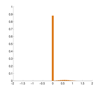
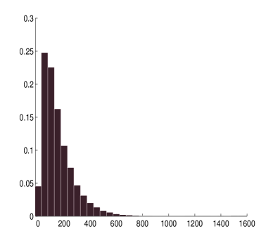
Figure 7: Simulation Results for Section 4.1, Simulation Two a) Histogram of 100,000 Values of $\mu$ Drawn from the Posterior $\pi(\mu,v)$, b) Histogram of Corresponding Backward Coupling Times

(a)                    (b)

4.2 A Two-Sample Problems

We now consider the model

$$Y_{ij}=\mu_{i}+\epsilon_{ij},\qquad i=1,2,\,\,\,\mbox{and}\,\,\,j=1,2,\ldots,n_{i},$$

where the $\epsilon_{ij}$ are all independent and

$$\epsilon_{ij}\sim N(0,v_{i})\qquad\mbox{for}\,\,\,i=1,2,$$

though other error distributions may easily be substituted.

Suppose that we wish to test

$$H_{0}:\mu_{1}=\mu_{2}$$

versus

$$H_{1}:\mu_{1}\neq\mu_{2},$$

in the cases where

1. $v_{1}$ and $v_{2}$ are fixed and known,

2. $v_{1}=v_{2}$ are unknown and given an inverse gamma prior, and

3. $v_{1}\neq v_{2}$ are unknown and given independent inverse gamma priors.

We consider a mixture prior density for $\mu=(\mu_{1},\mu_{2})$ that allows for the two components to possibly be equal:

$$f(\mu_{1},\mu_{2}|p,\theta_{1},\theta_{2})=p\cdot\delta_{0}(\mu_{1}-\mu_{2})\cdot f_{1}(\mu_{1}|\theta_{1})+(1-p)\cdot f_{2}(\mu_{1},\mu_{2}|\theta_{2})$$ (10)

with known hyperparameters $p$, $\theta_{1}$, and $\theta_{2}$.

The above cases can all be handled by our class coupler algorithm.

Case 1: $v_{1}$ and $v_{2}$ are fixed and known

We use the transition candidate density

$$q(\mu,\mu^{\prime})=q((\mu_{1},\mu_{2}),(\mu_{1}^{\prime},\mu_{2}^{\prime}))=\left\{\begin{array}[]{lcl}f_{2}(\mu_{1}^{\prime},\mu_{2}^{\prime}|\theta_{2})&,&\mbox{if}\,\,\,\mu_{1}=\mu_{2}\\ \\ \delta_{0}(\mu_{1}^{\prime}-\mu_{2}^{\prime})\cdot f_{1}(\mu_{1}^{\prime}|\theta_{1})&,&\mbox{if}\,\,\,\mu_{1}\neq\mu_{2}.\\ \end{array}\right.$$

Then the acceptance probability ratio is

$$r(\mu,\mu^{\prime})=\frac{\pi(\mu^{\prime})q(\mu^{\prime},\mu)}{\pi(\mu)q(\mu,\mu^{\prime})}=\frac{f(\vec{y}|\mu^{\prime})f(\mu^{\prime}|p,\theta_{1},\theta_{2})q(\mu^{\prime},\mu)}{f(\vec{y}|\mu)f(\mu|p,\theta_{1},\theta_{2})q(\mu,\mu^{\prime})}.$$

If we define

$$\mbox{class I}=\{(\mu_{1},\mu_{2}):\mu_{1}=\mu_{2}\}$$

and

$$\mbox{class II}=\{(\mu_{1},\mu_{2}):\mu_{1}\neq\mu_{2}\},$$

then we can be assured that all class I points $\mu=(\mu_{1},\mu_{2})$ will accept the class II candidate $\mu^{\prime}=(\mu_{1}^{\prime},\mu_{2}^{\prime})$ with probability

$$\begin{array}[]{lcl}\min_{\mu}\,r(\mu,\mu^{\prime})&=&\min_{\mu}\,\frac{f(\vec{y}|\mu^{\prime})(1-p)\cdot f_{2}(\mu_{1}^{\prime},\mu_{2}^{\prime}|\theta_{2})\cdot\delta_{0}(\mu_{1}-\mu_{2})\cdot f_{1}(\mu_{1}|\theta_{1})}{f(\vec{y}|\mu)\cdot p\cdot\delta_{0}(\mu_{1}-\mu_{2})f_{1}(\mu_{1}|\theta_{1})\cdot f_{2}(\mu_{1},\mu_{2}|\theta_{2})}\\ \\ &=&\min_{\mu}\,\frac{1-p}{p}\cdot\frac{f(\vec{y}|\mu^{\prime})}{f(\vec{y}|\mu)}.\end{array}$$

The minimum occurs when $\mu$ is the restricted MLE,

$$\hat{\mu}_{0}=\left(\frac{1}{n_{1}+n_{2}}\sum_{i=1}^{2}\sum_{j=1}^{n_{i}}Y_{ij},\frac{1}{n_{1}+n_{2}}\sum_{i=1}^{2}\sum_{j=1}^{n_{i}}Y_{ij}\right).$$

Similar calculations show that all class II points will accept the class I candidate $\mu$ with probability $r(\hat{\mu},\mu)$ where $\hat{\mu}$ is the unrestricted MLE given by

$$\hat{\mu}=\left(\frac{1}{n_{1}}\sum_{i=1}^{n_{1}}Y_{1i},\frac{1}{n_{2}}\sum_{i=1}^{n_{2}}Y_{2i}\right).$$

Therefore, we may run the same algorithm as in Section 4.1.

Case 2: $v_{1}=v_{2}$ are unknown and given an inverse gamma prior

We will use $v$ to denote the common value of $v_{1}$ and $v_{2}$. We assume an inverse gamma prior:

$$v\sim IG(k_{1},k_{2})$$

where $k_{1}$ and $k_{2}$ are known hyperparameters, and we assume that the $\mu=(\mu_{1},\mu_{2})$ and $v$ are a priori independent.

We choose the transition candidate density

$$\begin{array}[]{lcl}q((\mu,v),(\mu^{\prime},v^{\prime}))&=&q((\mu_{1},\mu_{2},v),(\mu_{1}^{\prime},\mu_{2}^{\prime},v^{\prime}))\\ \\ &=&\left\{\begin{array}[]{lcl}f_{2}(\mu_{1}^{\prime},\mu_{2}^{\prime}|\theta_{2})\cdot IG(v;k_{1},k_{2})&,&\mbox{if}\,\,\,\mu_{1}=\mu_{2}\\ \\ \delta_{0}(\mu_{1}^{\prime}-\mu_{2}^{\prime})\cdot f_{1}(\mu_{1}^{\prime};\theta_{\mu})\cdot IG(v^{\prime};k_{1},k_{2})&,&\mbox{if}\,\,\,\ \mu_{1}\neq\mu_{2}.\\ \end{array}\right.\end{array}$$

The acceptance probability ratio is

$$\begin{array}[]{lcl}r((\mu,v),(\mu^{\prime},v^{\prime}))&=&\frac{\pi(\mu^{\prime},v^{\prime})q((\mu^{\prime},v^{\prime}),(\mu,v))}{\pi(\mu,v)q((\mu,v),(\mu^{\prime},v^{\prime}))}\\ \\ &=&\frac{f(\vec{y}|\mu^{\prime},v^{\prime})f(\mu^{\prime}|p,\theta_{1},\theta_{2})IG(v^{\prime};k_{1},k_{2})q((\mu^{\prime},v^{\prime}),(\mu,v))}{f(\vec{y}|\mu,v)f(\mu|p,\theta_{1},\theta_{2})IG(v;k_{1},k_{2})q((\mu,v),(\mu^{\prime},v^{\prime}))}.\end{array}$$

If we define

$$\mbox{class I}=\{(\mu_{1},\mu_{2},v):\mu_{1}=\mu_{2}\}$$

and

$$\mbox{class II}=\{(\mu_{1},\mu_{2},v):\mu_{1}\neq\mu_{2}\},$$

then we can be assured that all class I points $(\mu,v)=(\mu_{1},\mu_{2},v)$ will accept the class II candidate $(\mu^{\prime},v^{\prime})=(\mu_{1}^{\prime},\mu_{2}^{\prime},v^{\prime})$ with probability

$$r((\hat{\mu}_{0},\hat{v}_{0}),(\mu^{\prime},v^{\prime}))$$

where $\hat{\mu}_{0}$ and $\hat{v}_{0}$ are the restricted MLEs

$$\hat{\mu}_{0}=\left(\overline{\overline{Y}},\overline{\overline{Y}}\right)=\left(\frac{1}{n_{1}+n_{2}}\sum_{i=1}^{2}\sum_{j=1}^{n_{i}}Y_{ij},\frac{1}{n_{1}+n_{2}}\sum_{i=1}^{2}\sum_{j=1}^{n_{i}}Y_{ij}\right)$$

and

$$\hat{v}_{0}=\frac{1}{n_{1}+n_{2}}\sum_{i=1}^{2}\sum_{j=1}^{n_{i}}(Y_{ij}-\overline{\overline{Y}})^{2}.$$

Similarly, all class II points $(\mu,v)$ will accept the class I candidate $(\mu^{\prime},v^{\prime})$ with probability

$$r((\hat{\mu},\hat{v}),(\mu^{\prime},v^{\prime}))$$

where $\hat{\mu}$ and $\hat{v}$ are the unrestricted MLEs

$$\hat{\mu}=(\overline{Y}_{1},\overline{Y}_{2})=\left(\frac{1}{n_{1}}\sum_{j=1}^{n_{1}}Y_{1j},\frac{1}{n_{2}}\sum_{j=1}^{n_{2}}Y_{2j}\right)$$

and

$$\hat{v}^{2}=\frac{1}{n_{1}+n_{2}}\left[\sum_{i=1}^{n_{1}}(Y_{1i}-\overline{Y}_{1})^{2}+\sum_{j=1}^{n_{2}}(Y_{2j}-\overline{Y}_{2})^{2}\right].$$

Case 3: $v_{1}\neq v_{2}$ are unknown and given independent inverse gamma priors

The prior for $(\mu,v)=(\mu_{1},\mu_{2},v_{1},v_{2})$ is

$$f(\mu|p,\theta_{1},\theta_{2})\cdot IG(\sigma_{1}^{2};k_{11},k_{12})\cdot IG(\sigma_{2}^{2};k_{21},k_{22})$$

where $f_{\mu}(\mu;\theta_{\mu})$ is from (10) and $k_{11},k_{12},k_{21}$, and $k_{22}$ are known hyperparameters.

We choose the transition candidate density

$$q((\mu,v),(\mu^{\prime},v^{\prime}))=q((\mu_{1},\mu_{2},v_{1},v_{2}),(\mu_{1}^{\prime},\mu_{2}^{\prime},v_{1}^{\prime},v_{2}^{\prime}))$$

$$=\left\{\begin{array}[]{lcl}f_{2}(\mu_{1}^{\prime},\mu_{2}^{\prime};\theta_{2})\cdot IG(v_{1}^{\prime};k_{11},k_{12})\cdot IG(v_{2}^{\prime};k_{21},k_{22})&,&\mbox{if}\,\,\,\mu_{1}=\mu_{2}\\ \\ \delta_{0}(\mu_{1}^{\prime}-\mu_{2}^{\prime})\cdot f_{1}(\mu_{1}^{\prime}|\theta_{1})\cdot IG(v_{1}^{\prime};k_{11},k_{12})\cdot IG(v_{2}^{\prime};k_{21},k_{22})&,&\mbox{if}\,\,\,\ \mu_{1}\neq\mu_{2}.\\ \end{array}\right.$$

The acceptance probability ratio is

$$\begin{array}[]{lcl}r((\mu,v),(\mu^{\prime},v^{\prime}))&=&\frac{\pi(\mu^{\prime},v^{\prime})q((\mu^{\prime},v^{\prime}),(\mu,v))}{\pi(\mu,v)q((\mu,v),(\mu^{\prime},v^{\prime}))}\\ \\ &=&\frac{f(\vec{y}|\mu^{\prime},v^{\prime})f(\mu^{\prime}|p,\theta_{1},\theta_{2})IG(v_{1}^{\prime};k_{11},k_{12})IG(v_{2}^{\prime};k_{21},k_{22})q((\mu^{\prime},v^{\prime}),(\mu,v))}{f(\vec{y}|\mu,v)f(\mu|p,\theta_{1},\theta_{2})IG(v_{1};k_{1},k_{2})IG(v_{2};k_{21},k_{22})q((\mu,v),(\mu^{\prime},v^{\prime}))}.\end{array}$$

Defining class I and class II points in the same way as in Case 2 above, we are assured that all class I points $(\mu,v)=(\mu_{1},\mu_{2},v_{1},v_{2})$ will accept the class II candidate $(\mu^{\prime},v^{\prime})=(\mu_{1}^{\prime},\mu_{2}^{\prime},v_{1}^{\prime},v_{2}^{\prime})$ with probability

$$r((\hat{\mu}_{0},\hat{v}_{0}),(\mu^{\prime},v^{\prime})$$

where $\hat{\mu}_{0}$ and $\hat{v}_{0}$ are the restricted MLEs

$$\hat{\mu}_{0}=\left(\overline{\overline{Y}},\overline{\overline{Y}}\right)=\left(\frac{1}{n_{1}+n_{2}}\sum_{i=1}^{2}\sum_{j=1}^{n_{i}}\ Y_{ij},\frac{1}{n_{1}+n_{2}}\sum_{i=1}^{2}\sum_{j=1}^{n_{i}}Y_{ij}\right)$$

and

$$\hat{v}_{0}=\left(\frac{1}{n_{1}}\sum_{i=1}^{n_{1}}(Y_{1i}-\overline{\overline{Y}})^{2},\frac{1}{n_{2}}\sum_{j=1}^{n_{2}}(Y_{2j}-\overline{\overline{Y}})^{2}\right).$$

Similarly, all class II points $(\mu,v)=(\mu_{1},\mu_{2},v_{1},v_{2})$ will accept the class I candidate $(\mu^{\prime},v^{\prime})=(\mu_{1}^{\prime},\mu_{2}^{\prime},v_{1}^{\prime},v_{2}^{\prime})$ with probability

$$r((\hat{\mu},\hat{v}),(\mu^{\prime},v^{\prime}))$$

where $\hat{\mu}$ and $\hat{v}$ are the unrestricted MLEs

$$\hat{\mu}=(\overline{Y}_{1},\overline{Y}_{2})=\left(\frac{1}{n_{1}}\sum_{j=1}^{n_{1}}Y_{1j},\frac{1}{n_{2}}\sum_{j=1}^{n_{2}}Y_{2j}\right)$$

and

$$\hat{v}=\left(\frac{1}{n_{1}}\sum_{i=1}^{n_{1}}(Y_{1i}-\overline{Y}_{1})^{2},\frac{1}{n_{2}}\sum_{j=1}^{n_{2}}(Y_{2j}-\overline{Y}_{2})^{2}\right).$$

References

- [1] J.M. Bernardo and R. Rueda. Bayesian Hypothesis Testing: A Reference Approach. International Statistical Review, 70:351-372, 2002.
- [2] H. Cai. A Note on an Exact Sampling Algorithm and Metropolis-Hastings Markov Chains. Technical report, University of Missouri, St. Louis, 1997.
- [3] G. Casella and M. Lavine and C. Robert. Explaining the Perfect Sampler. The American Statistician, 55:299-305, 2000.
- [4] J.N. Corcoran and R.L. Tweedie. Perfect Sampling of Ergodic Harris Chains. Annals of Applied Probability, 11(2):438-451, 2001.
- [5] J.N. Corcoran and R.L. Tweedie. Perfect Sampling From Independent Metropolis-Hastings Chains. Journal of Statistical Planning and Inference, 104(2):297-314, 2002.
- [6] J.A. Fill. An Interruptible Algorithm for Perfect Sampling via Markov Chains. Annals of Applied Probability, 8:131-162, 1998.
- [7] S.G. Foss and R.L. Tweedie. Perfect Simulation and Backward Coupling. Stochastic Models, 14:187-203, 1998.
- [8] S.G. Foss and R.L. Tweedie and J.N. Corcoran. Simulating the Invariant Measures of Markov Chains Using Horizontal Backward Coupling at Regeneration Times. Probability in the Engineering and Informational Sciences, 12:303-320, 1998.
- [9] R. Gottardo and A.E. Raftery. Markov Chain Monte Carlo with Mixtures of Singular Distributions. Technical Report no. 470, Department of Statistics, University of Washington, 2004.
- [10] P.J. Green Reversible Jump Markov Chain Monte Carlo Computation and Bayesian Model Determination. Biometrika, 82: 771-732, 1995.
- [11] O. Häggström and M.N.M. van Liesholt and J. Møller. Characterisation Results and Markov Chain Monte Carlo Algorithms Including Exact Simulation for Some Spatial Point Processes. Bernoulli, 5:641-659, 1999.
- [12] R.E. Kass and A.E. Raftery Bayes Factors. Journal of the American Statistical Association, 90:773-795, 1995.
- [13] W.S. Kendall. Perfect Simulation for the Area-Interaction Point Process. In Probability Towards the Year 2000, Springer, New York. Editors L. Accardi and C.C. Heyde. 218-234, 1998.
- [14] K.L. Mengersen and R.L. Tweedie. Rates of Convergence of the Hastings and Metropolis Algorithms. Annals of Statistics,24:101-121, 1996.
- [15] N. Metropolis, A. Rosenbluth, M. Rosenbluth, A. Teller, and E. Teller. Equations of State Calculations by Fast Computing Machines. Journal of Chemical Physics, 21:1087-1091, 1953.
- [16] S. P. Meyn and R. L. Tweedie. Markov Chains and Stochastic Stability, Springer-Verlag, London, 1993.
- [17] J. Møller. Perfect Simulation of Conditionally Specified Models. Journal of the Royal Statistical Society, Series B, 61(1):251-264, 1999.
- [18] D.J. Murdoch and P.J. Green. Exact Sampling from a Continuous State Space. Scandinavian Journal of Statistics, 25:483-502, 1998.
- [19] J.G. Propp and D.B. Wilson. Exact Sampling with Coupled Markov Chains and Applications to Statistical Mechanics, Random Structures and Algorithms, 9:223-252, 1996.
- [20] A.E. Raftery. it Hypothesis Testing and Model Selection, in Markov Chain Monte Carlo in Practice, Chapman & Hall. Editors W.R¿ Gilks and S. Richardson and D.J. Spiegelhalter. 163-187,1996.
- [21] G.O. Roberts and J.S. Rosenthal. Harris Recurrence of Metropolis-Within-Gibbs and Trans-Dimensional Markov Chains. Preprint available at http://www.statslab.cam.ac.uk/ ¡/horde/util/go.php?url=http mcmc , 2006
- [22] O. Stramer and R.L. Tweedie. Langevin-Type Models II: Self-Targeting Candidates for MCMC Algorithms. Methodology and Computing in Applied Probability, 1:307-328, 1999.
- [23] W. K. Hastings. Monte Carlo Sampling Methods using Markov chains and Their Applications. Biometrika, 57:97-109, 1970.
- [24] L. Tierney. Markov Chains for Exploring Posterior Distributions (with discussion). Annals of Statistics, 1:1701-1762, 1994.