The Cosmic History of Hot Gas Cooling and Radio AGN Activity in Massive Early-Type Galaxies

Abstract

We study the X-ray properties of 393 optically selected early-type galaxies (ETGs) over the redshift range of $z\approx$ 0.0–1.2 in the Chandra Deep Fields. To measure the average X-ray properties of the ETG population, we use X-ray stacking analyses with a subset of 158 passive ETGs (148 of which were individually undetected in X-ray). This ETG subset was constructed to span the redshift ranges of $z=$ 0.1–1.2 in the $\approx$4 Ms CDF-S and $\approx$2 Ms CDF-N and $z=$ 0.1–0.6 in the $\approx$250 ks E-CDF-S where the contribution from individually undetected AGNs is expected to be negligible in our stacking. We find that 55 of the ETGs are detected individually in the X-rays, and 12 of these galaxies have properties consistent with being passive hot-gas dominated systems (i.e., systems not dominated by an X-ray bright Active Galactic Nucleus; AGN). On the basis of our analyses, we find little evolution in the mean 0.5–2 keV to $B$-band luminosity ratio ($L_{\rm X}/L_{B}\propto[1+z]^{1.2}$) since $z\approx 1.2$, implying that some heating mechanism prevents the gas from cooling in these systems. We consider that feedback from radio-mode AGN activity could be responsible for heating the gas. We select radio AGNs in the ETG population using their far-infrared/radio flux ratio. Our radio observations allow us to constrain the duty cycle history of radio AGN activity in our ETG sample. We estimate that if scaling relations between radio and mechanical power hold out to $z\approx 1.2$ for the ETG population being studied here, the average mechanical power from AGN activity is a factor of $\approx$1.4–2.6 times larger than the average radiative cooling power from hot gas over the redshift range $z\approx$ 0–1.2. The excess of inferred AGN mechanical power from these ETGs is consistent with that found in the local Universe for similar types of galaxies.

1 Introduction

The most successful theoretical models of galaxy evolution (e.g. Bower et al. 2006 and Croton et al. 2006) require that feedback, in the form of energetic outflows from active galactic nuclei (AGNs), will have a fundamental influence on the evolution of intermediate and massive galaxies. In these models, energy injected from AGN radio jets heats the interstellar and intergalactic mediums of massive early-type galaxies (ETGs) and further drives interstellar gas out of these systems. This energy injection effectively quenches star formation and supermassive black hole (SMBH) accretion and prevents galaxies and SMBHs growing. The interstellar gas itself is thought to be produced by evolving stars ejecting material through stellar winds and supernovae (at a rate of $\approx 1.3[L_{B}/10^{11}L_{B,\odot}]M_{\odot}yr^{-1}$; e.g., Mathews & Brighenti 2003 and Bregman & Parriott 2009), as well as gas infall from the intergalactic medium.

The hot gas in massive ETGs ($\;\buildrel>\over{\sim}\;$$10^{11}M_{\odot}$) has been found to radiate powerfully at X-ray wavelengths through thermal bremsstrahlung and yet it does not appear to be cooling as expected. The X-ray spectral energy distributions (SEDs) of massive ETGs demonstrate that hot gas ($kT=$ 0.3–1 keV) typically dominates the 0.5–2 keV emission (e.g., Boroson et al. 2011). The temperatures and densities in the central regions imply relatively short radiative cooling times of $\approx 10^{8}$ yr (Mathews & Brighenti 2003). However, large quantities of cool ($10^{4-5}$K) gas are not observed in the ETGs, which would be predicted by simple cooling flow models (see, e.g., Mathews & Brighenti 2003 for a review). By these observational arguments, it is necessary that some feedback mechanism (e.g., the AGN radio jets predicted by the models) keeps the gas hot and/or expels the cooled gas reservoirs.

Direct observational evidence for the interaction of AGN radio jets with hot gas has been obtained via X-ray and radio observations of massive ETGs in the local universe (e.g., Boehringer et al. 1993; Bîrzan et al. 2004; Forman et al. 2005; Rafferty et al. 2006). These observations have revealed relativistic radio outflows inflating large X-ray-emitting gas cavities with cool gas observed at the cavity rims. Measurements of X-ray cavity sizes and their surrounding gas densities and temperatures can give estimates of the mechanical energy input required by the radio jets to inflate the cavities against the pressure of the surrounding gas. The derived mechanical energy and jet power are in the ranges $10^{55}$–$10^{62}$ ergs and $10^{40}$–$10^{46}$ erg s^-1, respectively (McNamara et al. 2009, Nulsen et al 2007; astro-ph/0611136), sufficient to suppress gas cooling in the galaxy and impede star formation and cold gas SMBH accretion (Allen et al. 2006). This type of feedback has been referred to as ‘radio mode’ or ‘maintenance mode,’ since during this phase the accretion rate onto the central SMBH driving the AGN is low, and thus the majority of the gas heating is through radio AGN activity.

These previous studies clearly indicate that heating by radio jets is an important process in galaxy evolution. Investigations of the influence of radio AGN on gas cooling in the general ETG population (Best et al. 2005; hereafter B05) found that more than 30% of the most massive ($\sim 5\times 10^{11}$M_⊙) galaxies host a radio AGN, which is consistent with radio AGN activity being eposidic with duty cycles of $\approx$$10^{7}$–$10^{8}$ yr (Best et al., 2006). Evidence of such episodic radio luminous activity is also implied by the presence of multiple bright rims and shocks in the X-ray and radio images of individual ETGs (e.g., M87; Forman et al. 2005). Therefore the prevention of the cooling of large quantities of gas is thought to be maintained by a self-regulating AGN feedback loop. Cooling gas in the ETG centre initially provides a slow deposition of fuel for SMBH accretion, which in a radiatively-inefficient accretion mode, leads to the production of a radio outburst. Surrounding cool gas is physically uplifted by the radio outbursts, which increases the gravitational potential energy of the gas or removes it from the system entirely (e.g. Giodini et al. 2010). As the gas further cools via X-ray emission, it falls back towards the SMBH where it can re-ignite a new cycle of accretion, thus completing the feedback loop (Best et al. 2006; McNamara & Nulsen 2007). The importance of the role of feedback from moderately radio luminous AGN is becoming increasingly apparent, since the feedback energy can be directly diffused into the interstellar medium (Smolčić et al., 2009).

A more complete understanding of the history of gas cooling and feedback heating in the massive ETG population requires direct X-ray and radio observations, respectively, of distant ETG populations covering a significant fraction of cosmic history. At present, such studies are difficult due to the very deep X-ray observations required to detect the hot X-ray emitting gas in such distant populations (however, see, e.g., Ptak et al. 2007 and Tzanavaris & Georgantopoulos 2008 for some early work). Notably, Lehmer et al. (2007) utilised X-ray stacking techniques and the $\approx$250 ks Extended Chandra Deep Field South (E-CDF-S) and $\approx$1 Ms Chandra Deep Field-South CDF-S to constrain the evolution of hot gas cooling (via soft X-ray emission) in optically luminous ($L_{B}\lower 2.15277pt\hbox{$\;\buildrel>\over{\sim}\;$}10^{10}$ $L_{B,\odot}$) ETGs over the redshift range of $z\approx$ 0–0.7. This study showed that the mean X-ray power output from optically luminous ETGs at $z\approx 0.7$ is $\approx$1–2 times that of similar ETGs in the local universe, suggesting the evolution of the hot gas cooling rate over the last $\approx$6.3 Gyr is modest at best. Considering the relatively short gas cooling timescales for such ETGs ($\sim$$10^{8}$ yr), this study provided indirect evidence for the presence of a heating source. Lehmer et al. (2007) found rapid redshift evolution for X-ray luminous AGNs in the optically luminous ETG population, which given the very modest evolution of the hot gas cooling, suggests that AGN feedback from the radiatively-efficient accreting SMBH population is unlikely to be the mechanism providing significant feedback to keep the gas hot over the last $\approx$6.3 Gyr. However, the mechanical feedback from radio AGNs, which is thought to be an important AGN feedback component, was not measured.

In this paper, we improve upon the Lehmer et al. (2007) results in the following key ways: (1) we utilise significantly improved spectroscopic and multiwavelength photometric data sets to select hot gas dominated optically luminous ETGs (via rest-frame colours, morphologies, and spectroscopic/photometric redshifts) and sensitively identify AGN and star-formation activity in the population (see $\S$ 2 and 3); (2) we make use of a larger collection of Chandra survey data (totaling a factor of $\approx$4 times the Chandra investment used by Lehmer et al. 2007) from the $\approx$2 Ms Chandra Deep Field-North (CDF-N; Alexander et al. 2003), the $\approx$4 Ms CDF-S (Xue et al. 2011), and the $\approx$250 ks E-CDF-S (Lehmer et al. 2005) (collectively the CDFs), which allows us to study the properties of hot gas (e.g., luminosity and temperature) in optically luminous ETGs to $z\approx 1.2$; and (3) we make use of new radio data from the VLA to measure the radio luminous AGN activity and the evolution of its duty cycle in the ETG population and provide direct constraints on the radio jet power available for feedback. The paper is organised as follows. In $\S$ 2, we define our initial working sample and discuss the ancillary multiwavelength data used to identify non-passive ETG populations. In $\S$ 3, we use various selection criteria to identify passive ETGs and ETGs hosting radio AGNs. In $\S$ 4, we constrain the evolution of the X-ray emission from hot gas in our passive ETG sample using X-ray stacking techniques. In $\S$ 5, we discuss the level by which radio AGN can provide heating to the hot gas in the ETG population. Finally, in $\S$ 6, we summarize our results. Throughout this paper, we make use of Galactic column densities of $N_{\rm H}$$=1.6\times 10^{20}$ cm^-2 for the CDF-N (Lockman 2004) and $N_{\rm H}$$=8.8\times 10^{19}$ cm^-2 for the E-CDF-S region (which also includes the CDF-S; Stark et al. 1992). In our X-ray analyses, we make use of photometry from 5 bands: the full band (FB; 0.5-8 keV), soft band (SB; 0.5-2 keV), soft sub-band 1 (SB1; 0.5-1 keV), soft sub-band 2 (SB2; 1-2 keV) and hard band (HB; 2-8 keV). The following constants have been assumed, $\Omega_{\rm M}=0.3$, $\Omega_{\rm\Lambda}=0.7$ and $H_{0}=70$ km s^-1Mpc^-1 implying a lookback time of 8.4 Gyr at $z=1.2$. Throughout the paper, optical luminosity in the $B$-Band ($L_{\rm B}$) is quoted in units of $B$-band solar luminosity ($L_{\rm B,\odot}=5.2\times 10^{32}$ erg s^-1).

2 Early-Type Galaxy Sample Selection

Figure 1: (a): Histogram of the entire sample of sources after imposing the selection criteria (i) to (iii) in $\S$ 2, showing the bimodal distribution of late-type and early-type galaxies. The dashed line shows the Bell et al. (2004) colour-cut, whereas the solid line shows the cut that we apply, slightly offset due to our different selection methods, using the redshift dependency taken from Bell et al. (2004) but varying the constant. The dotted and solid curves correspond to fitting a double gaussian to the sample in order to separate out the late and early-type populations, where the solid curve is the combination of the two gaussians. (b): Rest frame $U-V$ colour versus absolute (Vega) $V$-band magnitude. The small filled grey circles represent the whole orginal sample of sources, again after imposing the selection criteria (i) to (iii) in $\S$ 2 (including both ETGs and LTGs). The open symbols represent the 393 sources in our final sample of ETGs and the dotted lines represent the colour cut applied using the minimum source redshift and maximum source redshift in our sample, with the line for the median redshift shown as a solid line (this cut was then applied to our model data later in Fig. 4).

The primary goals of this study are to constrain the potential heating from AGN activity and the cooling of the hot gas in the optically luminous (massive) ETG population over the redshift range $z=$ 0.0–1.2 (i.e., over the last 8.4 Gyr). To achieve these goals optimally, we constructed samples of optically luminous ETGs in the most sensitive regions of the CDFs.

We began our galaxy selection using master optical source catalogues in the CDF-N and E-CDF-S, which contain a collection of IR–to–optical photometric data and good redshift estimates (either spectroscopic redshifts or photometric redshifts). The CDF-N master source catalogue consists of 48,858 optical sources detected across the entire CDF-N region (see Rafferty et al. 2011). This catalogue is based on optical sources detected in the Hawaii HDF-N optical and near-IR catalogue from Capak et al. (2004), and includes cross-matched photometry from GOODS-N through $HST$ ACS and $Spitzer$ IRAC catalogues (e.g., Giavalisco et al. 2004), $GALEX$ photometry, and deep $K_{s}$-band imaging (Barger et al., 2008). In the E-CDF-S, we made use of a master catalogue of 100,318 sources (see Rafferty et al. 2011). This catalogue is based on the MUSYC (Gawiser et al. 2006), COMBO-17 (Wolf et al. 2004), and the GOODS-S (Grazian et al. 2006) optical surveys, and includes cross-matched photometry from MUSYC near-IR (Taylor et al. 2009), SIMPLE $Spitzer$ IRAC (Damen et al. 2011), $GALEX$ (see footnote 1), and GOODS-S deep $U$-band photometry (Nonino et al. 2009). Our master catalogs are estimated to be complete to R$\leq 26$ (see section 2.1 of Xue et al. 2010).

Whenever possible, we utilised secure spectroscopic redshifts, which were collected from a variety of sources in the literature and incorporated into the master source catalogues discussed above. When spectroscopic redshifts were not available, we made use of high-quality photometric redshifts, which were calculated by Rafferty et al. (2011) using an extensive library of spectral templates (appropriate for galaxies, AGNs, hybrid galaxy and AGN sources, and stars), the optical–to–near-IR photometry discussed above, and the Zurich Extragalactic Bayesian Redshift Analyzer (ZEBRA; Feldmann et al. 2006). We compared these redshifts to the photometric redshift catalogue of Cardamone et al. (2010) finding a median difference of 0.01$\pm 0.16$ between $z=0.0-0.8$ and 0.01$\pm 0.32$ between $z=0.8-1.2$ in the two catalogues, thus providing additional evidence for the validity of these redshifts.

Starting with the master catalogues of 149,176 collective CDF sources, we imposed a series of selection criteria that led to the creation of our optically luminous ETG catalogue that we use throughout this paper; the imposed selection criteria are summarized below:

1. We restricted ETG catalogue inclusion to sources with $HST$ optical magnitudes of $z_{850}<23$ that were measured to be cosmologically distant (i.e., $z>0.05$). The requirement of $z_{850}<23$ ensures that the photometric redshifts of the remaining sources are of high quality and provides a highly optically complete (see Fig. 2) sample of relatively bright optically luminous ETGs out to $z\approx 1.2$. Note that these photo-zs were computed using a redshift training procedure that implements spectroscopic redshifts. The true accuracy of the photometric redshifts is expected to be $<$ 6-7 times worse than those available for sources with spectroscopic redshifts (see Luo et al. 2010 for details). This requirement further restricts our study to sources where $HST$ imaging is available, thus allowing for further visual inspection of the optical morphologies to reasonably good precision (see criterion v below). This criterion restricted our working sample to 9732 CDF sources.

2. We required that the sources are located within 6′ of at least one of the six independent $Chandra$ aimpoints in the CDFs (i.e., the $\approx$4 Ms CDF-S, four $\approx$250 ks E-CDF-S pointings, and $\approx$2 Ms CDF-N). This criterion ensures that the galaxies are located in regions where the $Chandra$ imaging is most sensitive and of highest quality (e.g., in these regions the $Chandra$ point-spread function is small and relatively symmetric). Applying this additional restriction led to a working sample consisting of 6446 CDF sources.

3. Using the redshift information available, we restricted our galaxy sample to include only sources with $z=0.05-1.2$. The upper redshift limit corresponds to the maximum distances to which we could obtain a complete sample of optically luminous ETGs that were relatively bright ($z_{850}<23$) and contain useful morphological information from HST imaging (see also, e.g., Häussler et al. 2007). Furthermore, this redshift upper limit for our survey allows us to detect the majority of X-ray luminous AGNs with $L_{\rm 2-8~{}keV}\geq 10^{42}$ erg s^-1 located in the $\approx$2 Ms CDF-N and $\approx$4 Ms CDF-S surveys. This therefore defines the redshift baseline over which we can reliably measure hot gas emission through X-ray stacking without significant impact from undetected AGNs (see $\S$ 4). As we will discuss below, when performing X-ray stacking analyses, we further exclude galaxies with $z\leq 0.6$ in the more shallow $\approx$250 ks E-CDF-S based on the same logic. For the moment, however, our galaxy sample includes E-CDF-S sources with $z\approx$ 0.6–1.2, since we will later use these galaxies to constrain the radio AGN duty cycle in the ETG populations (see $\S$ 5.1). The imposed redshift limits led to the inclusion of 5734 galaxies with $z=0.05-1.2$.

4. Since we are ultimately interested in measuring the hot gas X-ray emission from massive ETGs, we required that the galaxies that make up our sample have rest-frame $B$-band luminosities in the range of $L_{B}=$ 3–30 $\times 10^{10}L_{\rm B,\odot}$. As noted by O’Sullivan et al. (2001; see also Ellis & O’Sullivan 2006 and Boroson et al. 2011), such optically luminous ETGs in the local Universe have relatively massive dark matter halos, and are therefore observed to have 0.5–2 keV emission dominated by hot interstellar gas ($kT\lower 2.15277pt\hbox{$\;\buildrel>\over{\sim}\;$}$ 0.3–1 keV) with minimal contributions from other unrelated X-ray emitting sources (e.g., low-mass X-ray binaries; see Fig. 3b). This further restriction on including only optically luminous galaxies led to 2431 galaxies.

5. To identify passive ETGs in our sample, we made use of the multiwavelength photometry and redshift information discussed above to measure rest-frame $U-V$ colours, and we further used $HST$ imaging to provide morphological information about our galaxies. As noted by Bell et al. (2004), the rest-frame $U-V$ colour straddles the 4000 Å break and provides a sensitive indication of mean stellar age. For our sample, we first required that all galaxies have rest-frame $U-V$ colours redder than

   $$(U-V)_{\rm rest}=1.15-0.31z-0.08(M_{V}+22.4),$$ (1)

   where $M_{V}$ is the absolute $V$-band magnitude. Equation 1 (established to be valid out to $z\sim 1$) is based on Bell et al. (2004; see $\S$ 5); however we have used a different constant term based on our analysis in Fig. 1a where we determine the red/blue galaxy bimodal division by fitting a double gaussian to the distribution of $U-V+0.31z+0.08M_{V}$ for our sample of galaxies after imposing the selection criteria (i) to (iii). In this exercise, we applied the redshift dependency from Bell et al. (2004) but shifted the constant (by $\sim$$-0.13$) to fit to our sample, which is consistent with a typical colour scatter of $<0.2$ mag for the red sequence colour-magnitude relation (see $\S$ 4 in Bell et al. 2004). We classified galaxies lying below this divide as ‘blue cloud’ galaxies and those above as ‘red sequence’ galaxies. We (A.L.R.D. and B.D.L.) then visually inspected all red-sequence galaxies using grayscale HST images from the $z_{850}$ band, and for the subset of sources located in the GOODS-N and GOODS-S footprints, we also inspected HST false-colour images based on $B_{435}$, $V_{606}$, and $z_{850}$ observations. We strictly required the galaxies to have bulge dominant optical morphologies for ETG catalogue inclusion, and we rejected ETG candidates that appeared to be possible edge-on spirals, which may simply be reddened by intrinsic galactic dust. Furthermore, we removed five sources which were very near the edges of the HST images, where morphological classification was not possible. Applying these morphological criteria led to our final sample of 393 optically luminous ETGs. The basic properties of our parent sample are shown in Table 1.

Table 1: Master Catalogue.

RA	Dec	z	spec/phot?	z850	MU	MB	MV	LB	M∗	X-ray?	1.4GHz?	24$\mu$m?
(J2000)	(J2000)							log(LB,⊙)	log(M⊙)
(1)	(2)	(3)	(4)	(5)	(6)	(7)	(8)	(9)	(10)	(11)	(12)	(13)
52.8483000	-27.9371400	0.816	p	21.52	-21.79	-22.06	-22.83	11.01	11.16	0	0	0
52.8506205	-27.9442900	1.056	p	21.79	-21.41	-21.78	-22.36	10.91	11.00	0	0	0
52.8527205	-27.7069500	0.526	p	20.62	-20.49	-20.83	-21.65	10.52	10.84	0	0	0
52.8637605	-27.6886300	0.908	p	21.32	-21.22	-21.79	-22.53	10.91	11.29	0	0	0
52.8672000	-28.0023100	0.727	p	21.78	-20.64	-20.96	-21.55	10.57	10.73	0	0	0
52.8714105	-28.0047900	0.727	p	20.82	-21.33	-21.56	-22.24	10.81	11.04	0	0	0
52.8717405	-27.9800800	0.771	p	21.81	-21.25	-21.55	-22.15	10.81	10.88	0	0	0
52.8731805	-28.0159400	0.685	p	20.95	-20.95	-21.33	-22.23	10.72	11.10	0	1	0
52.8741105	-28.0181600	0.727	p	21.64	-20.81	-20.99	-21.67	10.59	10.80	0	0	0
52.8809595	-27.7222000	1.005	p	22.21	-21.27	-21.40	-21.98	10.75	11.02	0	0	0

Notes: Columns (1)–(2): Optical J2000 coordinates. Column (3): Source redshift. Column (4): s=spectroscopic redshift, p=photometric redshift. Column (5): z₈₅₀ magnitude. Column (6): U-band magnitude. Column (7): B-band magnitude. Column (8): V-band magnitude. Column (9): Logarithmic $B$-band optical luminosity (log($L_{B,\odot}$)). Column (10): Logarithmic stellar mass derived from K-band magnitude (log(M_⊙)). Column (11): Indicates whether the source was X-ray detected or not (0=not detected, 1=detected). Column (12): Indicates whether the source was 1.4GHz radio detected or not (0=not detected, 1=detected). Column (13): Indicates whether the source was 24$\mu$m detected or not (0=not detected, 1=detected). Table 1 is presented in its entirety (393 sources) in the electronic version of the journal. Only a portion (first 10 sources) is shown here for guidance.

We note that out of the 393 optically luminous ETGs that make up our sample, 190 of these galaxies lie in the CDF-S or CDF-N at $z=0.05$–1.2, or in the E-CDF-S at $z=0.05$–0.6, which could potentially be used in X-ray stacking. The remaining 203 sources lie in the E-CDF-S at $z=0.6$–1.2. Of the 393 galaxies in our sample, 163 have spectroscopic redshifts, and the remaining 230 sources have high-quality photometric redshifts from the Rafferty et al. (2011) catalogue. Furthermore, 128 out of 190 sources potentially to be used in X-ray stacking have spectroscopic redshifts.

Using both the photometric and spectroscopic redshifts we carry out a basic test of the environment of our sources by searching for neighbouring galaxies with an angular separation of $<$500kpc from each of our 393 ETGs and within a redshift difference of 0.09 and 0.046 in the CDF-N and E-CDF-S respectively (the dispersion in the photometric redshifts; see footnote 3). We first apply the cut in $z_{850}$ optical magnitude of $z_{850}<23$ in order to ensure we are only using high quality photometric redshifts and apply a further cut in absolute magnitude of M${}_{z850}<-21$. This results in a total galaxy sample of $\sim 3500$ galaxies in the CDF-N and $\sim 1000$ in the E-CDF-S. We find a median of $10\pm 1$ and $4\pm 2$ companions per ETG in the CDF-N and E-CDF-S respectively. We then check the number of neighbours we find for a random galaxy by searching within the comparison galaxy catalogues, and find a slightly lower median number of companions within 500kpc of $7\pm 2$ and $3\pm 1$ for the CDF-N and E-CDF-S respectively. Therefore, we find tentative evidence that the massive ETGs are in richer than average environments (likely small groups). Since we are using the photometric redshifts there is quite a large uncertainty, however, when using only the spectroscopic redshifts (giving us a much smaller and likely imcomplete sample) we do still find evidence for clustered environments. This is not unexpected since we are selecting massive ETGs.

Figure 2: The optical $B$-band luminosity of the ETG sample versus the redshift. The entire sample of 5734 sources after imposing the selection criteria (i) to (iii) in $\S$ 2 is represented by filled grey circles with the final ETG sample of 393 galaxies as open circles. The boxed areas show the bins from which sources were selected for X-ray stacking analysis, described in $\S$ 4.1. The bins were selected to be evenly separated in co-moving volume.

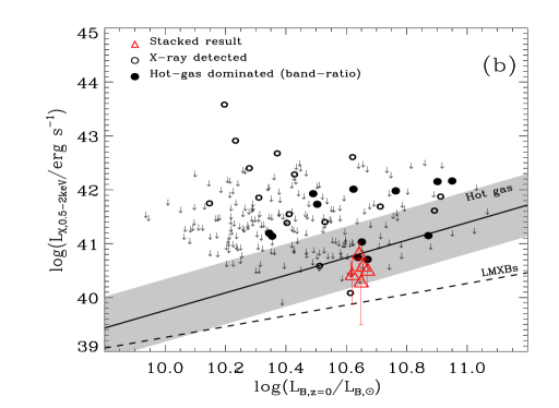
Figure 3: (a): The ratio of count-rates in the SB2 and SB1 X-ray bands against redshift. The solid line at $\Gamma_{\rm eff}=2.3$ shows our adopted divide between hot-gas dominated sources and possible low mass X-ray binary (LMXB) and/or AGN dominated sources. The SED for a 1.5 keV Raymond-Smith plasma (Raymond & Smith 1977) is shown as a dashed curve. Our stacked results (open triangles) are consistent with this SED. The errors on the band ratio were determined following the ‘numerical method’ described in $\S$ 1.7.3 of Lyons (1991). Band ratios are corrected for differential vignetting between the different bands using the appropriate exposure maps. (b): The rest-frame k-corrected SB (0.5–2 keV) X-ray luminosity (derived from the 0.5–1 keV flux to minimise contribution from LMXBs, and converted to 0.5–2keV luminosity using a 1.5 keV Raymond-Smith plasma SED) versus the faded, rest-frame $B$-band luminosity (where the evolution of $L_{B}$ is removed, using Faber et al. (2007) to parameterise the effect: $L_{\rm B,z=0}=L_{\rm B}\times 10^{-0.4\times 1.23\times z}$). The solid line and the 1$\sigma$ dispersion (shaded) show the contribution to X-ray emission from hot gas (O’Sullivan et al. 2001; converted from bolometric to soft-band X-ray luminosity). The dashed line represents the expected contribution to X-ray emission from LMXBs (O’Sullivan et al. 2001); arrows represent the 3$\sigma$ upper limit X-ray luminosities. Those sources identified as hot-gas dominated from their band ratios are represented here as filled circles, and they lie well within 3$\sigma$ of the hot gas relation from O’Sullivan et al. (2001). The results from the stacking procedure in six redshift bins are shown as open triangles and these results are based on the SB1 (0.5–1 keV) emission, convolved with the SED of a 1.5 keV Raymond-Smith plasma (Raymond & Smith 1977) to determine the corresponding SB (0.5–2 keV) emission.

Table 2: Hot gas dominated X-ray detected galaxies.

RA	Dec	z	SB1 counts	SB2 counts	SB2/SB1	LX,SB	$L_{1.4GHz}$	log(LB,z=0)	stack(y/n)
(J2000)	(J2000)		(0.5–1keV)	(1–2keV)		$10^{41}$erg s-1	$10^{22}\mu$Jy	log(LB,⊙)
(1)	(2)	(3)	(4)	(5)	(6)	(7)	(8)	(9)	(10)
03:32:09.706	$-$27:42:48.110	0.727	74.36${}^{+12.16}_{-10.98}$	125.44${}^{+15.84}_{-14.67}$	1.44${}^{+0.31}_{-0.26}$	185.79${}^{+30.38}_{-27.43}$	56.54$\pm$2.79	10.90	N
03:32:28.734	$-$27:46:20.298	0.737	61.89${}^{+9.56}_{-8.37}$	95.67${}^{+11.59}_{-10.41}$	1.52${}^{+0.30}_{-0.26}$	10.17${}^{+1.57}_{-1.38}$	59.63$\pm$2.81	10.62	Y
03:32:34.342	$-$27:43:50.092	0.668	40.22${}^{+8.36}_{-7.14}$	52.90${}^{+9.85}_{-8.64}$	1.22${}^{+0.35}_{-0.29}$	5.19${}^{+1.08}_{-0.92}$	$<$5.39	10.50	Y
03:32:38.786	$-$27:44:48.923	0.736	8.96${}^{+5.14}_{-3.85}$	$<$15.31	$<$1.61	1.51${}^{+0.87}_{-0.65}$	13.10$\pm$1.42	10.34	Y
03:32:41.406	$-$27:47:17.185	0.685	7.97${}^{+4.82}_{-3.51}$	8.41${}^{+4.99}_{-3.69}$	1.02${}^{+1.00}_{-0.59}$	1.06${}^{+0.64}_{-0.47}$	$<$5.72	10.65	Y
03:32:44.088	$-$27:45:41.461	0.488	8.70${}^{+5.15}_{-3.86}$	11.10${}^{+5.88}_{-4.62}$	1.20${}^{+1.14}_{-0.67}$	0.49${}^{+0.29}_{-0.22}$	$<$2.56	10.67	Y
03:32:46.536	$-$27:57:13.104	0.770	25.31${}^{+9.69}_{-8.50}$	37.30${}^{+11.75}_{-10.58}$	1.12${}^{+0.67}_{-0.44}$	68.68${}^{+26.29}_{-23.08}$	$<$7.55	10.95	N
03:32:46.949	$-$27:39:02.916	0.152	24.77${}^{+8.11}_{-6.90}$	$<$25.36	$<$0.73	1.32${}^{+0.43}_{-0.37}$	0.65$\pm$0.04	10.64	Y
03:32:52.066	$-$27:44:25.044	0.534	17.67${}^{+7.97}_{-6.76}$	23.03${}^{+9.58}_{-8.39}$	1.13${}^{+0.84}_{-0.54}$	17.88${}^{+8.07}_{-6.84}$	15.66$\pm 1.29$	10.87	Y
12:36:39.760	62:15:47.832	0.848	14.42${}^{+5.37}_{-4.21}$	$<$11.56	$<$0.86	8.41${}^{+3.13}_{-2.45}$	$<$6.34	10.49	Y
12:36:44.414	62:11:33.347	1.013	12.11${}^{+5.16}_{-3.89}$	14.00${}^{+5.37}_{-4.21}$	1.22${}^{+0.75}_{-0.52}$	9.27${}^{+3.95}_{-2.98}$	876.37$\pm 28.74$	10.76	Y
12:36:52.895	62:14:44.152	0.321	35.05${}^{+7.37}_{-6.21}$	44.53${}^{+8.11}_{-6.95}$	1.35${}^{+0.38}_{-0.32}$	1.34${}^{+0.28}_{-0.24}$	6.41$\pm 0.31$	10.35	Y

Notes: Columns (1)–(2): Optical J2000 coordinates. Column (3): Source redshift. Column (4): (0.5–1 keV) net counts. Column (5): (1–2 keV) net counts. Column (6): (1–2 keV)/(0.5–1 keV) count-rate ratio (SB2/SB1). Column (7): Rest-frame 0.5–2 keV luminosity (ergs s^-1) derived from SB1 counts and Raymond-Smith plasma SED. Column (8): Radio luminosity ($L_{\rm 1.4~{}GHz}$). Column (9): Logarithm of the $B$-band optical luminosity ($\log L_{B,\odot}$), Column (10): Indicates whether the source was included in our stacking analyses (Y/N).

3 Multiwavelength Characterisations of ETGs Using Ancillary Data

In this section, we make use of the extensive multiwavelength data available in the CDFs to identify both passive and non-passive (e.g., star-forming and AGN) ETGs. In the next section ($\S$ 4), we will perform X-ray stacking analyses of the passive ETG population to measure directly the evolution of the mean hot gas emission. In the analyses below, we match our 393 optically luminous ETG optical source positions to those provided in multiwavelength catalogues using closest-counterpart matching, which is a reasonable method provided that the optimum matching radius is carefully selected. We selected the optimum matching radius for each multiwavelength catalogue by first performing matching using a 30″ matching radius and then observing the distribution of closest-counterpart matching offsets. For all catalogues discussed below (i.e. optical-x-ray, optical-radio, optical-infrared matching), we found the distribution of offsets to peak close to $\approx$0″, reach a minimum at $\approx$1$\aas@@fstack{\prime\prime}$5, and subsequently rise toward larger offsets due to spurious matches. A matching radius of 1$\aas@@fstack{\prime\prime}$5 was therefore adopted as the optimum matching radius for all but the radio catalogues, for which the positional errors are very small, therefore 1″was more appropriate. Matches were visually inspected to further ensure they were sensible. The number of spurious matches was determined for each data set analytically by calculating the ratio between the total area covered by the parent sample sources, each with 1$\aas@@fstack{\prime\prime}$5 or 1″matching radius ($\pi(1.5)^{2}\times 393\approx 2778$sq. arcsec or $\pi(1.0)^{2}\times 393\approx 1234$sq. arcsec respectively) and the total area of the CDFs (within 6′ of each pointing; 0.188 sq. degrees or 2436480 sq. arcsec). This ratio was then multiplied by the total number of sources in the multiwavelength catalogues that lie within 6′ of one of the Chandra aimpoints.

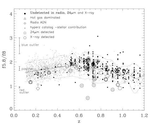
Figure 4: Selecting passive galaxies to use in the X-ray stacking analysis based on their IRAC 5.8 $\mu$m/8 $\mu$m colours. The solid curve shows the median 5.8 $\mu$m/8 $\mu$m colours of the 5000 model passive galaxy SEDs generated by hyperz with the 2$\sigma$ dispersion shown as dotted curves. In this figure, the most active galaxies (e.g. star-forming galaxies) have redder colours than those expected for passive ETGs. The error bars shown at $z=0.05$ are representative error bars, plotted at the median 5.8$\mu$m/8$\mu$m colour for the following three cases: sources lying within $\pm 2\sigma$ of the passive line; outliers with lower signal to noise with bluer colours ($>2\sigma$ above the passive line); redder AGN and active star-forming galaxies ($>2\sigma$ below the passive line). In our stacking analysis in $\S$ 4.1 we test the effect of including/not including the sources lying in regions which are $>2\sigma$ away from the passive line but which have not otherwise been classified as active, however, there is very little difference in the final result aside from signal-to-noise. In our final stacking analysis presented in Fig. 7 these sources have therefore been included.

3.1 X-ray Properties of ETGs

The ultradeep Chandra data in the CDFs provide a direct means for classifying X-ray detected ETGs as either hot gas dominated or likely AGNs. We used the published main catalogues for each of the CDFs, which consist of 503 sources in CDF-N ($\approx$2 Ms; $\approx$0.12 deg² survey, Alexander et al. 2003), 740 sources in the CDF-S ($\approx$4 Ms; $\approx$0.13 deg² survey, Xue et al. 2011), and 762 sources in the E-CDF-S (four contiguous $\approx$250 ks Chandra observations that flank the CDF-S proper; $\approx$0.31 deg², Lehmer et al. 2005). Using our sample of 393 ETGs, the optical coordinates of the galaxies were matched to the CDF X-ray catalogue positions using our adopted matching radius of 1$\aas@@fstack{\prime\prime}$5. When an ETG matched to a source in both the E-CDF-S and the CDF-S simultaneously (due to overlap between the E-CDF-S and CDF-S) we chose to use the data for the CDF-S, since these X-ray data are significantly deeper with smaller positional errors. In total, 55 X-ray matches were found once repetitions had been removed, including 11 in the CDF-N and 44 in the E-CDF-S region. The fraction of spurious matches in all the CDFs together was estimated to be $\approx$2.8% (or $\approx$2 expected spurious matches).

In Fig. 3a, we show the SB2/SB1 count-rate ratio versus redshift for the X-ray detected ETGs in our sample. The SB2/SB1 ratio provides an effective discriminator of the X-ray spectral shape in the SB, the energy regime where hot gas is expected to dominate. Typically, z$\approx 0$-2 AGNs have $\Gamma_{\rm eff}\sim 1.8$-2.3 (e.g., Alexander et al. 2005, Vignali et al. 2002, Reeves & Turner 2000). Therefore we took the upper limit of this range and conservatively classified sources with SB2/SB1 $\leq$ 1.7 (corresponding to $\Gamma_{\rm eff}\geq 2.3$) as sources having SB emission dominated by a hot gas component. Sources detected only in SB2 (i.e., having only a lower-limit on SB2/SB1), that had SB2/SB1 limits below our adopted cut were not classed as hot gas dominated sources. Sources with SB2/SB1 hardness ratio greater than this cut (i.e., SB2/SB1 $>1.7$), have X-ray emission likely dominated by low mass X-ray binaries (LMXBs) or X-ray AGNs. However, by construction, our choice to study optically luminous ETGs will inherently minimise contributions from LMXB-dominated systems and therefore AGNs are expected to dominate the SB2/SB1 $>1.7$ population (see below). Our SB2/SB1 criterion indicated 12 hot-gas dominated sources and 25 likely AGNs (Fig. 3a). The SB2/SB1 ratios imply that a Raymond-Smith plasma (Raymond & Smith 1977) of kT$\sim$1.5keV is a good spectral model from which to convert count-rates to flux. In Table 2, we tabulate the properties of these X-ray detected ETGs.

In Fig. 3b, we show the 0.5–2 keV luminosity (hereafter, $L_{\rm X}$) versus $L_{B,0}$ (see $\S$ 4 for details) for the ETGs in our sample. In order to minimise the contribution from LMXBs we calculated the rest-frame 0.5–2 keV luminosities $L_{\rm X,SB}$ based on the 0.5–1 keV SB1 fluxes provided in the Chandra catalogues and convert them to 0.5–2 keV SB fluxes, applying a k-correction:

$$L_{\rm X}=4\pi d_{\rm L}^{2}f_{\rm X}k\;\;\;({\rm erg~{}s^{-1}}),$$ (2)

where $d_{L}$ is the luminosity distance in cm, $f_{\rm X}$ is the 0.5–2 keV flux in units of erg cm^-2 s^-1. The quantity $k$ is the redshift-dependent k-correction. For sources that were characterised as hot gas dominated we used the observed 0.5–1 keV flux and a Raymond-Smith plasma SED (with $kT_{\rm X}=1.5$ keV; Raymond & Smith 1977; see Fig. 3a) to compute $L_{\rm X}$. For sources that were identified as AGN dominant, we used a power-law SED (with $\Gamma=1.8$) and the observed 0.5–2 keV flux to compute $L_{\rm X}$. The solid line and shaded region shows the best-fit local relation and 1$\sigma$ dispersion for hot gas dominated ETGs, and the dashed line shows the expected contribution from LMXBs (based on O’Sullivan et al. 2001 and typically a factor of $\sim$10 below the hot gas contribution). We note that nearly all ETGs without X-ray detections (plotted as upper limits) and the 12 ETGs with SB2/SB1 band ratios consistent with being hot gas dominated (highlighted with filled circles) also have $L_{\rm X}/L_{B}$ values similar to those observed for local hot gas dominated ETGs. The majority of the remaining X-ray detected sources with SB2/SB1 $>1.7$ are expected to be AGNs. As Fig. 3b shows, these sources typically have large values of $L_{\rm X}/L_{B}$, again consistent with that expected from AGNs (see O’Sullivan et al. 2001; Ellis & O’Sullivan 2006). To further check for AGNs in our sample we cross-matched our optical catalogue with spectroscopic data from Szokoly et al. (2004), Mignoli et al. (2005), Ravikumar et al. (2007), Boutsia et al. (2009) and Silverman et al. (2010) using a 1$\aas@@fstack{\prime\prime}$5 radius in order to identify any sources with spectral features indicative of AGN, such as broad emission lines. We identified two potential broad line AGN in the E-CDF-S, both of which were X-ray detected and had already been flagged as likely AGN using our band ratio analysis (Fig. 3).

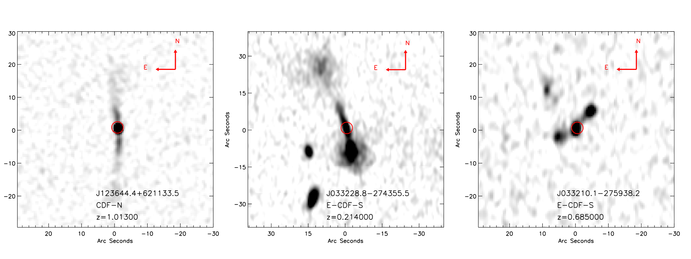
Figure 5: Radio images of the three extended radio matches discovered by visual inspection of the radio images. The axes give the distance to the centre of the image in arcseconds. All of these extended sources have significantly higher 1.4GHz fluxes (1.2–4.8mJy) than the other 16 radio-bright AGN in our ETG sample.

3.2 5.8–24 $\mu$m Properties of ETGs

In order to explore further whether the ETGs contained more subtle signatures of AGN or star-formation activity than provided by their X-ray and optical spectroscopic properties, we utilised Spitzer photometry over the 5.8–24 $\mu$m range. We began by using Spitzer IRAC 5.8 $\mu$m/8 $\mu$m colours. Since AGN tend to be redder than galaxies in the mid-infrared, the 5.8 $\mu$m/8 $\mu$m colour can be used to identify AGNs when the continuum is dominated by a rising power law component rather than a dropping stellar component (e.g., Stern et al. 2005). Similarly, the SEDs of powerful star-forming galaxies, containing a large hot dust component, may exhibit this rise towards redder wavelengths and may also be identified by their 5.8 $\mu$m/8 $\mu$m colour. In the E-CDF-S, we take the photometry in these channels from Damen et al. (2011) and in the CDF-N, we take photometry from GOODS-N, cutting both catalogues at a signal-to-noise level of S/N$<5$.

We matched the positions from our sample of 393 ETGs to the Spitzer IRAC catalogues using a matching radius of 1$\aas@@fstack{\prime\prime}$5 and found 384 matches. We estimated a spurious matching fraction of $\approx$3.1% ($\approx$12 matches). In Fig. 4, we show the 5.8 $\mu$m/8 $\mu$m colour versus redshift for the 384 ETGs in our main sample. To determine the expected 5.8 $\mu$m/8 $\mu$m colours for passive galaxies, we used the code hyperz (Bolzonella et al., 2000) with the SED library of Bruzual & Charlot (1993) to generate 5000 model galaxy SEDs based on a wide range of star formation histories and redshifts. For each galaxy, we adopted a formation redshift randomly selected to lie between the galaxy redshift (i.e., $t_{\rm age}=0$) and $z\approx 5$. In Fig. 4, we plot the running median of the 5.8 $\mu$m/8 $\mu$m colours for the hyperz sample, after imposing the rest-frame $U-V$ color criterion in equation 1 (the solid line in Fig. 4), and calculate the 2$\sigma$ dispersion either side of the median (the dashed lines on Fig. 4). This curve was calculated by binning the data into bins of $\Delta z=0.05$ and computing the median and dispersion for each bin. Sources with very red IRAC colours lying below the passive line are likely AGN or star forming galaxies, and it can be seen that X-ray, radio and 24 $\mu$m detected galaxies tend to lie below the solid line. In our stacking analyses (see $\S$ 4.1), we experimented with removing the sources that lie outside of the 2$\sigma$ dispersion boundaries of our hyper-z normal galaxy envelope. However, we found no difference in the general results since most of the sources exhibiting non-passive activity (either due to star formation or AGNs) had already been identified by other indicators, and we therefore decided to include all of our galaxies in our subsequent stacking analyses (unless otherwise flagged as non-passive). As an additional test we experimented with the IRAC colour-colour diagnostic as in Stern et al. (2005), Fig. 1, however, we find that only three of our sources lie in their region of active sources, all three of which we have already flagged as active sources through our other diagnostics.

To identify additional ETGs in our sample that have signatures of star formation or AGN activity from dust emission, we cross-matched our ETG sample with Spitzer MIPS 24 $\mu$m catalogues. The E-CDF-S was observed with Spitzer/MIPS as part of the FIDEL legacy program (PI: Mark Dickinson; see $\S$ 2.1.2–2.1.3 of Magnelli et al. 2009). We have used a catalogue of 20329 sources produced by the DAOPHOT package in IRAF (see $\S$ 2.3 of Biggs et al. 2011). The MIPS 24 $\mu$m sensitivity over the E-CDF-S varies significantly across the $30\arcmin\times 30\arcmin$ field, with exposure times ranging from 11,000–36,000 s. We make use of sources having signal-to-noise of at least 5$\sigma$ ($\approx$30–70 $\mu$Jy limits; see Magnelli et al. 2009). For the CDF-N, we made use of the publicly available GOODS Spitzer Legacy survey catalogues of 1198 sources (PI: M. Dickinson). We utilised the 5$\sigma$ sample (flux limits of 70 $\mu$Jy in the E-CDF-S and 30 $\mu$Jy in the CDF-N; Magnelli et al. 2009). Using a 1$\aas@@fstack{\prime\prime}$5 matching radius we found a total of 20 matches to the 393 ETGs in our sample; three in the CDF-N and 17 in the E-CDF-S, with $\sim$1.7 spurious matches expected. 24 $\mu$m provides a robust diagnostic of the presence of cold dust emission from the circumstellar envelopes of young embedded UV-luminous stars, characterised by a rising SED through the mid-infrared Muzerolle et al. (2004). Such systems are expected to contain significant X-ray contributions from populations that are unrelated to hot gas, and we therefore classify these 20 sources to be star-formation active systems.

3.3 Radio Properties of ETGs

To measure powerful radio emission produced by either radio-loud AGNs or star-formation activity, we cross-matched the optical coordinates of the parent sample with 1.4 GHz VLA catalogues in the CDFs (using a 1″ matching radius). We utilised the catalogue from Miller et al. (2008), but included additional sources at S/N$>$5 (Miller et al. in preparation) for the E-CDF-S region, which contains 940 radio sources with S/N$>5$ and reaches a 5$\sigma$ limiting flux density of 30 $\mu$Jy with a synthesised beam of 2.8″ $\times$ 1.6″. For the CDF-N, we utilised the catalogue from the Morrison et al. (2010) GOODS-N observations, which provides entries for 1227 discrete radio sources with S/N$>5$ and 5$\sigma$ flux density limit of 20 $\mu$Jy at the field centre, with a 1.7″ beam. In total, 24 radio detected counterparts to the 393 ETGs were found (six in the CDF-N and 18 in the E-CDF-S) and 15 of these radio detected ETGs were also X-ray detected. The spurious matching fraction was estimated to be $\approx$0.5% ($\approx$0.1 matches) and therefore negligible. Since the radio emission from radio luminous AGNs can be extended (e.g., Fanaroff & Riley 1974), the radio maps were carefully inspected by eye against the 1″ radius matching circles (overlaid at the locations of the parent sample positions) to verify the accuracy of the matches and isolate extended sources. We identified three bright extended sources that were all identified using closest-counterpart matching; radio images of these sources have been provided in Fig. 5. We note that some of these individual sources have been well studied in the literature (e.g. J123644.4; Richards et al. 1998, J033238.8 and J033210.1; Kellermann et al. 2008).

We calculated rest-frame 1.4 GHz monochromatic luminosities for all radio detected sources following,

$$L_{\rm 1.4~{}GHz}=4\pi d^{2}_{\rm L}f_{\rm 1.4GHz}10^{-36}(1+z)^{\alpha-1}{\rm W~{}Hz^{-1}},$$ (3)

where $f_{\rm 1.4~{}GHz}$ is the 1.4 GHz flux density ($\mu$Jy) and $\alpha$ is the radio spectral index for a power-law radio SED (i.e., $F_{\nu}\propto\nu^{-\alpha}$). We adopted a power-law spectral index of $\alpha=0.85$ (see Richards 2000 for motivation). For normal galaxies without active radio AGNs, radio emission originates from HII regions and Type II and Ib supernovae, which produce synchrotron radiation from relativistic electrons and free-free emission (Condon 1992). In passive ETGs, the contribution from these processes is unlikely to exceed $10^{18-19}$WHz^-1 (Ledlow 1997). The radio luminosity for all radio detected sources in our sample was greater than $10^{20}$ W Hz^-1, which is expected given the flux limits of our survey. Therefore, detecting them at all suggests an excess of non-passive activity from either star-formation (SFR $\lower 2.15277pt\hbox{$\;\buildrel>\over{\sim}\;$}0.1$ $M_{\odot}$ yr^-1) or AGN activity.

To discriminate between star-formation and AGN activity in the radio-detected population, we use the well-known strong correlation between radio and far-infrared emission, which extends to cosmologically significant redshifts (at least $z\approx 1$; Appleton et al. 2004, and z$>2$ using total infrared luminosity; Mao et al. 2011). For all our ETGs that are detected at both 24 $\mu$m and 1.4 GHz we measured the quantity $q_{24}\equiv\log(f_{24\mu m}/f_{\rm 1.4GHz})$ (Appleton et al., 2004) (where $f_{24\mu m}$ and $f_{\rm 1.4GHz}$ are observed fluxes). Radio-excess AGN can be identified by comparing their infrared emission to their radio emission, as their radio emission is significantly brighter than their infrared emission when compared to star-forming galaxies, which fit tightly along the far-infrared/radio correlation. Following Del Moro et al. (submitted) demonstrating the typical $q_{24}$ of radio-excess AGN based on starburst SEDs, we apply a selection of $q_{24}<0.5$ to be indicative of radio AGN. This results in 19 of the 24 radio-detected galaxies being classified as radio AGN, with the remaining five radio-detected galaxies being classified as star-forming galaxies (as indicated in Table 4). In this exercise 10 ETGs with 24 $\mu$m detections but not radio detections were excluded from the final sample. We note that 16 of the 24 radio AGN were also X-ray detected. Table 4 shows the matched radio sources that are classified as radio AGN from the q₂₄ analysis, and which are used to estimate the AGN heating in $\S$ 5. We note that this approach identified all the sources with extended radio emission in Fig. 5 as radio AGN.

In Table 3, we summarise the various source classifications described in $\S$ 3 for clarity. Of the original 393 galaxies in the ETG sample 190 of them can potentially be used in the X-ray stacking (see $\S$ 2). However, through various classification schemes we find that 32 of these are non-passive (potential X-ray AGN or star-forming galaxies) and are therefore excluded from the main stacking sample, thus leaving a sample of 158 passive galaxies which are suitable for X-ray stacking analyses. Of the 393 ETGs, 24 are radio detected and 20 of these are likely radio AGN while the other five have radio emission dominated by star formation. We classify a further 10 sources as likely star-forming galaxies, which have detections only in 24 $\mu$m and not radio, and lower limits of q${}_{24}>0.5$.

Table 3: Summary of source classifications.

Classification	No. of galaxies
ETG sample	393
X-ray detected	55
Passive X-ray detected	12
Potential LMXB/X-ray AGN	43
Radio detected	24
Radio AGN	19
24$\mu$m detected	20
Star-forming galaxies	15
X-ray stacked galaxies (main)	158
X-ray stacked galaxies (faded)	60

Figure 6: Ratio of observed flux in 24 $\mu$m and radio (1.4GHz) versus redshift. Sources which lie below the solid line (Del Moro et al, in prep) are taken to be radio AGN.

Table 4: Radio-bright ETGs.

RA	Dec	z	$f_{1.4\rm GHz}$	log(L1.4GHz)	$f_{\rm 24\mu m}$	q24	LX,SB	log(LB)	Extended	Note
(J2000)	(J2000)		($\mu$Jy)	($10^{23}$WHz-1)	($\mu$Jy)		($10^{42}$erg s-1cm-2)	(log(LB,⊙))	(Y/N)	(AGN/SF)
(1)	(2)	(3)	(4)	(5)	(6)	(7)	(8)	(9)	(10)	(11)
03:31:29.563	-28:00:57.384	0.685	46.3$\pm$8.8	0.9$\pm$0.2	$<$70	$<$0.18	…	10.7	N	A
03:31:32.210	-27:43:08.076	0.956	68.7$\pm$7.3	2.9$\pm$0.3	85.5$\pm$6.2	0.09	$<$5.1	10.9	N	A
03:31:39.041	-27:53:00.096	0.220	61.2$\pm$7.0	0.08$\pm$0.01	85.5$\pm$5.3	0.15	…	10.6	N	A
03:31:40.044	-27:36:47.628	0.685	208.1$\pm$15.4	4.0$\pm$0.3	$<$70	$<$-0.47	…	11.2	N	A
03:31:45.895	-27:45:38.772	0.727	42.7$\pm$6.8	0.9$\pm$0.2	$<$70	$<$0.22	…	11.3	N	A
03:31:57.782	-27:42:08.676	0.665	97.2$\pm$6.5	1.7$\pm$0.1	73.7$\pm$3.1	-0.12	8.4	10.8	N	A
03:32:09.706	-27:42:48.110	0.727	257.2$\pm$12.7	5.6$\pm$0.3	$<$70	$<$-0.57	18.6	11.3	N	A
03:32:10.137	-27:59:38.220	0.685	1165.0$\pm$36.0	22.2$\pm$0.7	$<$70	$<$-1.22	…	11.2	Y	A
03:32:19.305	-27:52:19.330	1.096	39.1$\pm$6.2	2.3$\pm$0.4	$<$70	$<$0.25	…	11.3	N	A
03:32:28.734	-27:46:20.298	0.737	263.3$\pm$12.4	6.0$\pm$0.3	$<$70	$<$-0.58	1.0	11.0	N	A
03:32:28.817	-27:43:55.646	0.214	4814.0$\pm$103.0	6.3$\pm$0.1	$<$70	$<$-1.84	0.04	10.6	Y	A
03:32:38.786	-27:44:48.923	0.736	58.0$\pm$6.3	1.3$\pm$0.1	247.8$\pm$2.4	0.63	0.2	10.7	N	S
03:32:39.485	-27:53:01.648	0.686	107.0$\pm$6.2	2.04$\pm$0.12	$<$70	$<$-0.18	$<$0.2	11.0	N	A
03:32:46.949	-27:39:02.916	0.152	105.5$\pm$7.0	0.060$\pm$0.004	106.2$\pm$2.7	0.003	0.1	10.7	N	A
03:32:48.177	-27:52:56.608	0.668	32.8$\pm$6.2	0.6$\pm$0.1	152.4$\pm$2.3	0.67	4.9	11.2	N	S
03:32:52.066	-27:44:25.044	0.534	148.3$\pm$12.2	1.6$\pm$0.1	$<$70	$<$-0.326	1.79	11.1	N	A
03:33:05.671	-27:52:14.268	0.521	55.7$\pm$6.8	0.6$\pm$0.1	181.5$\pm$7.6	0.51	$<$2.4	11.3	N	S
03:33:15.427	-27:45:24.012	0.727	63.5$\pm$6.9	1.4$\pm$0.2	368.3$\pm$2.7	0.76	…	10.6	N	S
12:36:01.813	62:11:26.659	0.913	99.2$\pm$5.5	3.8$\pm$0.2	$<$30	$<$-0.52	…	10.9	N	A
12:36:08.137	62:10:36.136	0.679	213.1$\pm$7.9	4.0$\pm$0.2	2300.0$\pm$12.9	1.03	0.2	10.7	N	S
12:36:17.098	62:10:11.554	0.846	65.3$\pm$8.3	2.1$\pm$0.3	88.2$\pm$6.4	0.13	7.95	10.7	N	A
12:36:22.705	62:09:46.313	0.748	45.7$\pm$5.1	1.1$\pm$0.1	$<$30	$<$-0.18	…	10.6	N	A
12:36:44.414	62:11:33.347	1.013	1805.1$\pm$59.2	87.6$\pm$2.9	$<$30	$<$-1.78	0.9	11.3	Y	A
12:36:52.895	62:14:44.152	0.321	198.3$\pm$9.6	0.64$\pm$0.03	$<$30	$<$-0.82	0.1	10.5	N	A

Notes: Columns (1)–(2): Optical J2000 coordinates. Column (3): Redshift. Column (4): Radio (1.4GHz) flux density ($\mu$Jy). Column (5): Radio (1.4 GHz) luminosity ($\log 10^{23}$W Hz^-1). Column (6): 24 $\mu$m flux density ($\mu Jy$). Column (7): $q_{24}$ ratio, ($\log f_{24\mu m}/f_{1.4GHz}$). Column (8): 0.5–2 keV flux ($10^{42}$ ergs s^-1 cm^-2) derived from SB1 (0.5–1 keV) counts and converted using the 1.5 keV Raymond-Smith plasma. Column (9): $B$-band luminosity ($\log L_{\rm B,\odot}$). Column (10): Indicates whether there is extended emission (Y=yes, N=no). Column (11): Note on classification: S = radio detected ETGs for which the radio emission is likely dominated by star formation (as implied by their $q_{24}$ value), A = radio emission dominated by an AGN.

4 Cosmic History of X-ray Emission from Massive ETGs

Approximately 90% of the ETGs in our passive sample are undetected in the X-ray (338 galaxies). Therefore to measure the hot gas emission from the whole population it is necessary to implement X-ray stacking techniques. This investigation focuses on measuring the cooling of the hot gas in ETGs, which dominates emission at soft X-ray energies (0.5–2 keV), as opposed to LMXBs, which dominate emission in the hard band (2–8 keV). Stacking analyses were therefore carried out in the soft bands (i.e., SB1 and SB2), which we expect to be dominated by hot-gas emission and to have minimal contributions from LMXBs. In Fig. 2, we plot six redshift intervals of galaxies with $L_{B}=(3-30)\times 10^{10}L_{B,\odot}$ where we performed stacking analyses for each subsample (solid boundaries). The redshift divisions were chosen to encompass roughly equal intervals of comoving volume, and the larger redshift interval spacing beyond $z\approx 0.6$ is the result of excluding from our stacking analyses sources that were within the $\approx$250 ks exposure of the E-CDF-S (see $\S$2 for details).

We note that previous studies (e.g., Bell et al. 2004; Faber et al. 2007) have shown that, from $z=1-0$, the $B$-band luminosity of typical massive ETGs fades by $\sim$1 mag. To estimate the mean X-ray luminosity evolution for an ETG population with similar $z=0$ $B$-band luminosities ($L_{B,z=0}$), we thus constructed six “faded” redshift-divided subsamples of ETGs with $L_{B,z=0}=(3-30)\times 10^{10}L_{B,\odot}$. We calculated $L_{B,z=0}$ following the Faber et al. (2007) prescription: $L_{B,z=0}=L_{B}\times 10^{-0.4\times 1.23\times z}$. With these faded luminosities only 60 of the 158 stacking sources lay within the allowed range of optical luminosities. In total, we stacked 12 subsamples of ETGs (six main and six faded) with both the main and faded samples having the same divides in redshift but with 158 sources in the total main sample and only 60 in the total faded sample.

4.1 X-ray Stacking Technique

Our stacking procedure, summarized below, makes use of images, background maps, and exposure maps that were constructed by Alexander et al. (2003) for the $\approx$2 Ms CDF-N, Lehmer et al. (2005) for the $\approx$250 ks E-CDF-S, and Xue et al. (2011) for the $\approx$4 Ms CDF-S.

We chose to use circular apertures of constant radii to extract on-source counts. We chose to extract X-ray counts (source plus background) from a 1$\aas@@fstack{\prime\prime}$5 radius circular aperture centered on the locations of sources that were within 6′ of any of the six Chandra aimpoints (the $\approx$2 Ms CDF-N, the $\approx$4 Ms CDF-S, and the four $\approx$250 ks pointings in the E-CDF-S). These choices of source inclusion radius and extraction aperture radius were previously found to optimise the stacked signal (see, e.g., Lehmer et al. 2005b, 2007) and are therefore implemented here. For each source, we used our source extraction aperture to extract source plus background counts $s_{i}$ from images and exposure times $t_{i}$ from exposure maps. For each stacked sample, total source plus background counts were computed as $S=\sum_{i}s_{i}$ and exposure times were computed as $T=0.03\sum_{i}t_{i}$ (the 0.03 factor comes from the fact that $t_{i}$ is the sum of exposure map values over $\approx$30 pixels).

Background and exposure maps were then used to measure the background counts and exposures for each source. For this exercise, we used a 15″ radius circular aperture centred on the location of each source to extract local background counts $b_{i,\rm local}$ and exposure times $t_{i,\rm local}$. The on-source background counts $b_{i}$, were estimated following $b_{i}=b_{i,\rm local}\times t_{i}/t_{i,\rm local}$. Total stacked background counts were then obtained through the summation $B=\sum_{i}b_{i}$.

For each stacked sample, any galaxy that was classified as a normal ETG (see $\S$3) was stacked. The stacking procedure was carried out with three different samples: (a) a sample including all radio AGN, passive X-ray detected sources (10 galaxies) and passive X-ray undetected sources; (b) a sample including only X-ray undetected galaxies and (c) a sample including passive X-ray undetected galaxies and radio AGN but excluding passive X-ray detected galaxies. However, we found that the inclusion of both X-ray detected normal galaxies and radio AGN in the stacking did not significantly change our results, implying that most X-ray luminous AGN had been successfully excluded from the sample via direct X-ray detection and classification. Therefore all radio AGN and X-ray detected normal galaxies (thus all passive galaxies) were included in all of the stacks resulting in a final sample of 158 and 60 passive ETGs to be stacked in the main and faded samples, respectively.

For each stacked sample, we measured the signal-to-noise ratio ($S/N=(S-B)/\sqrt{B}$). For a significant detection, we required that $S/N>3$, and for such stacks, we measured net counts as $N=S-B$. When a stacked sample was not detected, we placed 3$\sigma$ upper limits on the net counts i.e. $N<3\sqrt{\alpha_{S}^{2}+\alpha_{B}^{2}}$, where $\alpha_{S}$ and $\alpha_{B}$ are the bootstrapped errors on the total and background counts respectively. The error on the net counts was determined by applying a bootstrapping method. For each stacked sample containing $n$ galaxies, we randomly drew $n$ sources from the sample (allowing for multiple draws of the same source) and restacked the scrambled sample to measure net counts. This exercise was performed 1000 times for each stacked sample, thus giving a sense of the variance of the population. The count-rates $\Phi$ for each stacked sample were determined as $\Phi=\xi N/T$, where $\xi$ is a mean aperture correction. Since many of the sources with relatively large PSFs (at $\approx$3–6′ off axis) had aperture radii that did not encompass the whole PSF, it was necessary to factor in a correction ($\xi_{i}$) for each of the stacked sources. The average correction factor used was computed as $\xi\equiv\sum_{i}\xi_{i}t_{i}/\sum_{i}t_{i}$ where $\xi_{i}$ and $t_{i}$ are the correction factors and exposure times measured for each individual source. The stacked count-rates $\Phi$ were then converted to fluxes using the SED for a 1.5 keV Raymond-Smith plasma (Raymond & Smith 1977; see Fig. 3a for motivation and see Table 5 for kT_X values used in each stack sample). Errors on the count-rate to flux conversion were calculated by propagating errors on the mean SB2/SB1 ratio, which can be used as a proxy for temperature in our Raymond-Smith SED. The errors on the luminosity were determined by propagating the bootstrapped errors on the source counts and the errors on the countrate-to-flux conversion factor based on the errors in the SED temperature described above. When calculating luminosities, the luminosity distance is calculated using the mean redshift in each bin (since as Fig.  2 demonstrates, the redshifts are quite evenly distributed in each stacking bin).

Table 5: X-ray stacking properties.

				Exposure time
		Net counts (S-B)		SB1	SB2	S/N		fSB1	kTX	LX,SB	LB,mean	LX,SB/LB
zmean	Ntot	SB1	SB2	(Ms)	(Ms)	SB1	SB2	log(erg s-1cm-2)	(keV)	log(erg s-1)	log(LB,⊙)	log(erg s-1L${}_{B,\odot}^{-1}$)
(1)	(2)	(3)	(4)	(5)	(6)	(7)	(8)	(9)	(10)	(11)	(12)	(13)
					General Sample
0.278	19	80.7$\pm$42.2	125.3$\pm$66.3	12.2	12.3	29.3	36.4	-16.1	1.3${}^{+0.2}_{-0.1}$	40.7$\pm 0.2$	10.7	29.9$\pm 0.2$
0.519	19	38.8$\pm$20.3	55.0$\pm$28.1	25.7	26.3	9.9	11.1	-16.8	1.3${}^{+0.6}_{-0.1}$	40.6$\pm 0.2$	10.8	29.8$\pm 0.2$
0.630	33	58.2$\pm$40.5	97.3$\pm$50.2	85.2	85.5	7.7	10.2	-17.0	1.6${}^{+0.5}_{-0.4}$	40.5$\pm 0.3$	10.7	29.8$\pm 0.2$
0.790	43	112.6$\pm$59.0	178.8$\pm$93.5	111.6	111.6	12.7	16.5	-16.9	1.5${}^{+0.3}_{-0.3}$	40.9$\pm 0.2$	10.8	30.2$\pm 0.2$
0.973	32	35.4$\pm$12.9	43.5$\pm$17.8	71.7	71.6	5.0	5.1	-17.1	1.2${}^{+1.2}_{-0.1}$	40.9$\pm 0.2$	10.8	30.1$\pm 0.1$
1.124	12	6.1$\pm$4.8	9.4$\pm$6.8	34.7	34.7	1.3	1.5	$<$-17.2	…	$<$40.9	10.9	$<$30.1
					Faded Sample
0.284	13	29.3$\pm$23.2	32.0$\pm$24.3	6.2	6.4	15.8	13.3	-16.5	1.0${}^{+0.2}_{-0.1}$	40.3$\pm 0.3$	10.7	29.7$\pm 0.3$
0.518	11	35.1$\pm$17.6	51.9$\pm$24.5	17.6	18.2	10.9	13.0	-16.8	1.33${}^{+0.03}_{-0.45}$	40.5$\pm 0.2$	10.7	29.9${}^{+0.3}_{-0.2}$
0.632	13	49.4$\pm$34.9	79.4$\pm$48.4	37.3	37.7	9.8	12.6	-17.1	1.5${}^{+0.2}_{-0.6}$	40.4$\pm 0.3$	10.6	29.8$\pm 0.2$
0.767	15	105.8$\pm$54.9	151.0$\pm$85.2	41.7	41.7	19.4	22.3	-16.9	1.3${}^{+0.1}_{-0.4}$	40.8$\pm 0.2$	10.6	30.2$\pm 0.3$
0.980	5	16.5$\pm$8.5	18.4$\pm$9.6	13.4	13.3	5.4	4.8	-17.4	1.2${}^{+0.5}_{-0.4}$	40.6$\pm 0.2$	10.7	30.0$\pm 0.3$
1.119	3	2.6$\pm$3.1	2.8$\pm$1.4	9.6	9.6	1.0	0.8	$<$-17.5	…	$<$40.7	10.6	$<$30.0

Notes: Column (1): Mean redshift of bin. Column (2): Number of sources in stacking bin. Columns (3)–(4): Net counts for SB1 and SB2. Columns (5)–(6): Exposure times in Ms for SB1 and SB2. Columns (7)–(8): Stacked signal-to-noise ratio for SB1 and SB2. Column (9): Logarithm of the stacked SB1 flux (ergs s^-1 cm^-2). Column (10): X-ray temperature (keV). Column (11): Logarithm of the stacked 0.5–2 keV luminosity $L_{\rm X}$ (ergs s^-1) measured using the SB1 flux and an assumed Raymond-Smith plasma SED with 1.5 keV temperature. Column (12): Logarithm of the $B$-band luminosity (for the faded sample, we list $L_{B,z=0}$). Column (13) Logarithm of the 0.5–2 keV to $B$-band luminosity ratio (for the faded sample, we list $L_{\rm X}/L_{B,z=0}$).

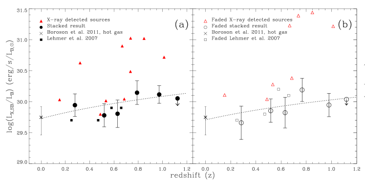
Figure 7: (a): The evolution of the soft X-ray properties of hot-gas dominated ETGs in terms of $B$-band optical luminosity, including passive X-ray detected galaxies, passive X-ray undetected galaxies and radio AGN. All galaxies with individual detections in the SB band are plotted as triangles. The circles represent the stacked results in six redshift bins with only an upper limit in the highest redshift bin. There is very little evolution of L_X,SB1/L_B in these hot gas dominated galaxies, in particular given the very short expected cooling time of hot gas. To minimise the contribution from LMXBs we stack in SB1 (0.5-1keV) but we use the SED of a 1.5keV plasma to convert this to SB (0.5-2keV) in order to more easily compare the data to previous studies. $z=0$ points are shown for the hot gas contribution as determined from a subset of the ETG sample of Boroson et al. (2011). The simple two-parameter fit for $\log L_{\rm X}/L_{\rm B}=A+B\log(1+z)$ is shown as a dotted curve on both panels (a) and (b), with best-fit values of [$A$,$B$] = [$29.73\pm 0.14$, $1.19\pm 0.68$] and [$29.71\pm 0.14$, $1.07\pm 0.68$] for the main and faded samples, respectively. (b): Represents the faded sample, showing that the fading of L_B with cosmic time is a fundamental effect and acts to slightly decrease the observed L${}_{\rm X,SB}/$L_B ratio with increasing redshift. The errors on the luminosity are derived from propagating the bootstrapped errors on the net counts and systematic errors on the conversion between count-rate and flux using the 1.5keV Raymond-Smith plasma SED.

4.2 X-ray Stacking Results

The results of stacking the X-ray data of the sample, are summarised in Table 5. In Figures 3a and 3b, we have overlaid our stacking results, demonstrating that our galaxies have SB2/SB1 count-rate ratios consistent with our adopted 1.5 keV Raymond-Smith plasma SED (which we use to convert count-rates to fluxes and luminosities) and $L_{\rm X}$ versus $L_{B,z=0}$ values consistent with local hot gas dominated ETGs. In Figures 7a and 7b, we display the rest-frame 0.5–2 keV luminosity (computed following equation 2) per $B$-band luminosity $L_{\rm X}$/$L_{B}$ versus redshift for our main and faded samples, respectively (circles). The 10 individually X-ray detected, hot gas dominated ETGs are shown as triangles in Figures 7a and 7b (only eight are shown on Fig. 7b as only eight fulfilled the constraints of the stacking for the faded sample). Only 10 out of the 12 galaxies shown in Table 2 are included in the stacking as, for stacking, we add the limitation that all galaxies in the E-CDF-S must have $z<0.6$. As would be expected from an X-ray selected subset, these sources generally have higher values of $L_{\rm X}/L_{B}$. For comparison, we have also plotted the mean $L_{\rm X}/L_{B}$ values obtained by Lehmer et al. (2007) for ETGs with $L_{B}>10^{10}$ $L_{B,\odot}$ (squares).

To constrain evolution to $z=0$, we take the Boroson et al. (2011) sample of 30 nearby ETGs and select only those 14 with $L_{B}=$ (3–30) $\times 10^{10}L_{\rm B,\odot}$. We convert their 0.3–8 keV luminosities to 0.5–2 keV luminosities using our adopted 1.5 keV Raymond-Smith plasma SED and find a mean value of $\log L_{\rm X}/L_{B}=$ 29.7 $\pm$ 0.2 (crosses in Figs. 7a and 7b). The combination of the Boroson et al. (2011) mean $L_{\rm X}/L_{B}$ and our stacking results indicates that there is little apparent evolution in $L_{\rm X}/L_{\rm B}$ for these optically luminous ETGs. However, a Spearman’s $\rho$ test reveals that the quantity $L_{\rm X}/L_{\rm B}$ is correlated with $z$ at the 92% and 96% probability level for the main and faded samples respectively. To constrain the allowable redshift evolution of $L_{\rm X}/L_{\rm B}$, we fit a simple two parameter model to the data $\log L_{\rm X}/L_{\rm B}=A+B\log(1+z)$ and find best-fit values of [$A$,$B$] = [$29.73\pm 0.14$, $1.19\pm 0.68$] and [$29.71\pm 0.14$, $1.07\pm 0.68$] for the main and faded samples, respectively. These values indicate mild evolution in the X-ray activity of luminous ETGs and are consistent with those of Lehmer et al. (2007). Using this model, we find that at z=1.2, ETGs are $\sim 2.4\pm 0.9$ times or $\sim 2.2\pm 0.9$ times (for the main and faded sample respectively) more X-ray luminous (per unit L_B) than at z=0, which suggests only modest evolution. Our best-fit relations have been highlighted in Figures 7a and 7b as dashed curves.

Since the stacked X-ray properties (i.e., SB2/SB1 band ratio and $L_{\rm X}$ versus $L_{B}$) are consistent with those expected from hot gas dominated ETGs, with little expected contributions from LMXBs, we can use the X-ray luminosity versus redshift diagram for our stacked samples as a direct tracer of the hot gas cooling history for massive ETGs with $L_{B}=(3-30)\times 10^{10}L_{B,\odot}$. The observed mild decline in X-ray luminosity per unit $B$-band luminosity and roughly constant X-ray gas temperature for massive ETGs over the last $\approx$8.4 Gyr of cosmic history suggest that, on average, the gas is being kept hot. We expect that many complex processes are contributing to the evolution of the gas including radiative cooling, periodic AGN heating and outflows, replenishment from stellar winds and supernovae, interactions and sloshing, and intergalactic medium and poor group inflow (e.g. Tabor & Binney 1993, Best et al. 2006, Faber & Gallagher 1976 and Brighenti & Mathews 1999). The detailed influences that each of these processes has on the gas are difficult to quantify, particularly without a strong idea of the environment in which each galaxy resides. However, we know that most of our sources reside within small groups and clusters, therefore, processes such as intergalactic medium and poor group infall may be important. One of the goals of this paper is to test whether AGN feedback from mechanical feedback can provide enough energy to keep the gas hot and counter the observed cooling over the long baseline of cosmic time spanned by our observations.

In the next section, we discuss the viability of AGN feedback heating of the gas by directly measuring the history of radio AGN events in our galaxy population and computing the mechanical energy available from these events.

5 Discussion

5.1 The Hot Gas Cooling and Mechanical Heating Energy Budgets

The above X-ray stacking results indicate that the X-ray power output from hot gas in the massive ETG population remains well regulated across a large fraction of cosmic history (since $z\sim 1$). To determine whether the heating from AGNs is sufficient to keep the gas hot, we estimated the mechanical power input from AGNs and the radiative cooling power from the hot gas. As discussed in $\S$ 4.2, the history of gas cooling power can be directly inferred from our X-ray stacking results; the gas cooling power, can be expressed as

$$L_{\rm cool}=C_{\rm bol}L_{\rm X}\approx C_{\rm bol}L_{B}10^{A}(1+z)^{B},$$ (4)

where $A=29.73\pm 0.14$ and $B=1.19\pm 0.68$ were computed in $\S$4.2, $L_{B}\approx 6.3\times 10^{10}$ $L_{B,\odot}$ is the mean value of $L_{B}$, and $C_{\rm bol}\approx 1.8$ is the bolometric correction for a hot gas SED with 1.5 keV temperature (see $\S$4.2 above). In Fig. 8, we plot the mean cooling history (filled circles and dashed curve for stacked values and best-fit model, respectively), since $z\approx 1.2$.

To estimate the energy input from radio AGNs over the last $\approx$8.4 Gyr of cosmic history, we began by measuring the radio AGN fraction as a function of radio luminosity (a proxy for mechanical heating) and redshift. By making the assumption that all galaxies will go through multiple AGN active phases, we can use the radio-luminosity and redshift dependent AGN fraction as a proxy for the typical AGN duty cycle history for galaxies in our sample.

To establish a baseline local ($z\approx 0$) measurement of the ETG radio AGN fraction, we used the B05 sample of radio-loud AGN from the SDSS survey, which included both early-type and late-type galaxies. For the sake of comparing these data with our ETG sample, we selected galaxies in the B05 sample with elliptical-like concentration indices $C>2.6$ (Strateva et al., 2001). The concentration index is defined as $C=r_{90}/r_{50}$, where $r_{90}$ and $r_{50}$ are radii containing 90% and 50% of the optical light respectively. By applying the flux density limit of 5 mJy, we limit the B05 sample to a lower radio luminosity limit of $\approx$$10^{23}$ W Hz^-1, which corresponds to a maximum redshift of $z=0.1$. To measure the AGN fraction for galaxies in the distant Universe, we used the sample of distant ETGs presented in this paper. Using $L_{\rm 1.4~{}GHz}=10^{23}$ W Hz^-1, the luminosity limit used for the B05 data, we determined that the corresponding CDF-N and E-CDF-S radio flux limits (see $\S$3.3) allow us to study similar AGNs out to $z\approx 1$ and 0.85, respectively. We calculated the AGN fraction for both the local B05 local galaxies and our distant galaxies in three bins of radio luminosity (in even logarithmic luminosity intervals) in the range of $L_{\rm 1.4~{}GHz}\sim(1-100)\times 10^{23}$ W Hz^-1, each bin with a different allowed redshift range due to the flux limits. These bins in luminosity and redshift then result in a total of 2642 elliptical galaxies containing a radio AGN from the B05 sample and 13 radio AGN from our sample. The AGN fraction was computed in each bin, for both the B05 sample and our sample, by taking the total number of radio AGN in a particular luminosity range and dividing it by the total number of galaxies in which an AGN with a luminosity lying within that range could have been detected if present. We estimate 1$\sigma$ errors on the AGN fractions following Gehrels (1986). By comparing the radio AGN fraction at the mean redshift $z=z_{\rm mean}$ of our distant galaxy sample with that of the B05 $z\approx 0$ sample, we can estimate the evolution of the duty cycle of the AGN outbursts in each radio luminosity bin. The time-dependent radio AGN fraction for each bin of radio-luminosity was computed following

$$f_{AGN}(t,L_{{\rm 1.4~{}GHz},i})=\frac{f_{{\rm AGN},z=z_{{\rm zmean},i}}-f_{{\rm AGN},z\approx 0,i}}{\Delta t_{i}}t+f_{{\rm AGN},z\approx 0,i},$$ (5)

where $\Delta t_{i}$ is the difference in the mean lookback time between $z=z_{{\rm mean},i}$ and $z=0$ (i.e., our AGN fraction and that of B05) in a particular bin of mean radio luminosity $L_{{\rm 1.4~{}GHz},i}$.

Several studies have now shown that the radio power output $L_{\rm 1..4~{}GHz}$ from AGNs within nearby giant elliptical (gE) and cluster central galaxies correlates with the inferred mechanical power $L_{\rm mech}$ that is needed to inflate the cavities within hot X-ray halos (e.g., Bîrzan et al. 2004; Bîrzan et al. 2008; Cavagnolo et al. 2010; O’Sullivan et al. 2011). Until recently, these relations have been calibrated using the cores of cooling clusters, and may not be appropriate for the massive early-type galaxies studied here. Cavagnolo et al. (2010) have added a sample of 21 gE galaxies and have shown that, as long as the radio structures are confined to the hot X-ray emitting gas region, gE galaxies provide a natural extension to the $L_{\rm mech}$–$L_{\rm 1.4~{}GHz}$ correlation at low $L_{\rm mech}$. However, as noted by Cavagnolo et al. (2010), gE galaxies and FRI sources in group environments (e.g., Croston et al. 2008) tend to have $L_{\rm mech}/L_{\rm 1.4~{}GHz}$ ratios much lower than the correlation derived including clusters. Since our galaxies are expected to be gE and group central galaxies, we made use of $L_{\rm mech}$ and $L_{\rm 1.4~{}GHz}$ values for the sample of 21 gEs from Cavagnolo et al. (2010) to derive the $L_{\rm mech}$–$L_{\rm 1.4~{}GHz}$ correlation for these sources. Figure 8 shows the 21 gEs from Cavagnolo et al. (2010). We find that the best-fit relation from Cavagnolo et al. (2010) (dashed line in Fig. 8), which includes radio galaxies at the centers of galaxies, overpredicts the $L_{\rm mech}/L_{\rm 1.4~{}GHz}$ ratios for AGNs with $L_{\rm 1.4~{}GHz}\lower 2.15277pt\hbox{$\;\buildrel>\over{\sim}\;$}10^{22}$ W Hz^-1. Using these data, we derived the following relation, which is applicable to gE galaxies:

$$L_{\rm mech}\approx 3.36\times 10^{35}\left(\frac{L_{\rm 1.4~{}GHz}}{10^{24}{\rm W~{}Hz^{-1}}}\right)^{0.11}{\rm W}.$$ (6)

Our best-fit relation is plotted in Figure 8 as a solid line.

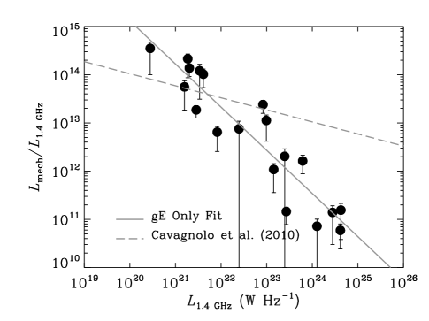
Figure 8: Ratio of mechanical power to 1.4 GHz radio luminosity ($L_{\rm mech}/L_{\rm 1.4~{}GHz}$) versus $L_{\rm 1.4~{}GHz}$ for the 21 giant elliptical (gE) galaxies studied by Cavagnolo et al. (2010; filled circles). The Cavagnolo et al. (2010) relation, which includes gE galaxies and radio galaxies at the centers of cooling clusters (from Bîrzan et al. 2008), has been shown as a dashed line. Our best-fit relation for gE only galaxies, presented in equation 6, is shown as a solid line.

Using equations (5) and (6), we then estimate the average mechanical feedback power per galaxy over the last $\approx$8.4 Gyr of cosmic history considering all radio AGNs in the range of $L_{\rm 1.4~{}GHz}\sim$ (1–100) $\times 10^{23}$ W Hz^-1 via the following summation:

$$L_{\rm heating}=\sum_{i}f_{AGN}(t,L_{{\rm 1.4~{}GHz},i})\;L_{\rm mech,i}$$ (7)

In Fig. 9, we show the mean heating luminosity and 1$\sigma$ errors (solid curve with shaded envelope) derived following equation 7. From Fig. 9, we see that on average there appears to be more than sufficient input mechanical energy from radio AGN events to balance the hot gas radiative cooling. From the five stacked bins where we obtain X-ray detections, we estimate on average $L_{\rm heating}/L_{\rm cool}\approx 2.4^{+0.9}_{-0.5}$. This result is broadly in agreement with that found for local elliptical galaxies of comparable mass where the mechanical power has been measured using X-ray cavities (e.g., Nulsen et al. 2007). Nulsen et al. (2007) estimate that the total cavity heating can be anywhere between 0.25 and 3 times the total gas cooling if 1 pV of heating is assumed per cavity; however, the enthalpy of the cavity and therefore the total heating may be much higher. Stott et al. (submitted) find a trend in groups and clusters indicating the ratio of intra-cluster medium (ICM) AGN heating (from the brightest cluster galaxy) to ICM cooling increases with decreasing halo mass. For halo masses $<5\times 10^{12}$M_⊙ the heating can exceed the cooling. We have found that most of our galaxies are likely to live in small group environments. Therefore extrapolating this relation to the expected halo masses of the galaxies in our sample ($\approx$[1–10] $\times 10^{12}M_{\odot}$ for $L_{B}\approx$ [3–30] $\times 10^{10}$ $L_{B,\odot}$; Vale & Ostriker 2004) would similarly imply that the mechanical heating would likely exceed the radiative cooling.

We note that our heating calculation is based on duty cycle histories derived primarily from the $<$20 distant radio AGNs in our sample and is based on the assumption that each galaxy will have many radio outbursts that span the full range of radio luminosities studied here. We therefore expect these calculations will have significant uncertainties that we cannot determine. In the next section, we estimate the global ETG hot gas cooling and radio AGN heating power as a function of redshift.

5.2 Cosmic Evolution of Global Heating and Cooling Density

Using a large sample of radio-loud AGNs in the local Universe, Best et al. (2006) computed the radio-luminosity and black-hole mass dependent AGN fraction of nearby galaxies. Their data show that the population-averaged mechanical power (probed by 1.4 GHz power) produced by these AGN events increases with black-hole mass (and also $B$-band luminosity) and balances well the radiative power output from X-ray cooling of the hot gas (see their Fig. 2). Their analyses further revealed that relatively low luminosity radio AGN ($\log L_{\rm 1.4~{}GHz}/({\rm W~{}Hz^{-1}})\approx$ 22–25) are likely to provide the majority of the mechanical feedback power for the population as a whole. They estimated that in the local universe, the mean mechanical power output density from mechanical heating from radio AGNs with $L_{\rm 1.4~{}GHz}>10^{22}{\rm W~{}Hz^{-1}}$ is $\approx$$4\times 10^{31}$ W Mpc^-3.

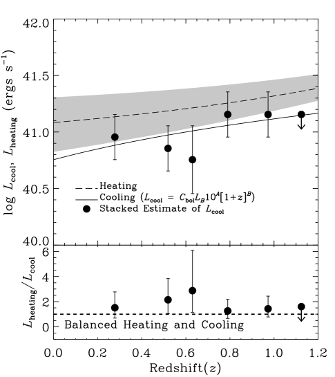
Figure 9: (top panel) Mean radiative cooling power $L_{\rm cool}$ and mean mechanical heating power $L_{\rm heating}$ versus redshift. The filled circles and 1$\sigma$ error bars show the bolometrically corrected estimates of $L_{\rm cool}$ (see Table 5) and the solid curve shows our best-fit model. The long-dashed curve with shaded region represents our best estimate of the mean heating luminosity as presented in equation 7. These measurements show that for the early-type galaxies in our sample, there is more than enough energy available from radio AGN heating to keep the gas from cooling. (bottom panel) Ratio of mean heating to radiative cooling luminosity versus redshift. We find that the average heating power is $\approx$1.4–2.6 times larger than the radiative hot gas cooling power.

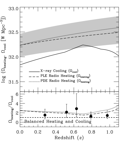
Figure 10: (top panel) Cosmic history of mechanical heating $\Omega_{\rm heating}$ and radiative cooling $\Omega_{\rm cool}$ of hot gas since $z\approx 1.1$. The mechanical luminosity density versus redshift for radio AGNs, as computed by Smolčić et al. (2009), for pure-luminosity evolution and pure density evolution are indicated as dashed and dotted curves, respectively. The shaded envelope provides the estimated uncertainties between the $L_{\rm 1.4~{}GHz}$ and $L_{\rm mech}$ correlation. The cooling history of hot gas in ETGs is indicated as a solid curve (see $\S$5.2 for details). (bottom panel) Ratio of mechanical heating to radiative cooling versus redshift. For comparison, we have plotted our estimates of the mean heating-to-cooling luminosity ratios ($L_{\rm heating}/L_{\rm cool}$ as provided in the bottom panel of Fig. 9 (filled circles). This relation shows that there is plenty of mechanical energy potential available to keep the gas hot over the last $\approx$8.4 Gyr.

Due to the relatively small number of radio AGNs found in our survey, it is not feasible to calculate the evolution of the radio and mechanical luminosity density of the Universe. However, the evolution of the radio AGN luminosity function has recently been measured out to $z\approx 1.3$ using the VLA-COSMOS survey (Schinnerer et al., 2007) to relatively faint luminosity levels ($L_{\rm 1.4~{}GHz}\lower 2.15277pt\hbox{$\;\buildrel>\over{\sim}\;$}10^{21}$–$10^{23}$ ${\rm W~{}Hz^{-1}}$; Smolčić et al. 2009). By converting radio luminosity into mechanical luminosity, Smolčić et al. (2009) integrated their luminosity functions to determine the estimated mechanical power density of the Universe out to $z\approx 1.3$. In Fig. 10, we show the expected mechanical feedback power density evolution, based on the Smolčić et al. (2009) radio luminosity function and equation 6 for both pure-luminosity density evolution ($L_{*}\propto[1+z]^{0.8}$) and pure-density evolution ($\Phi_{*}\propto[1+z]^{1.1}$), the best-fit parameterisations for the evolution of the 1.4 GHz luminosity function.

As shown in $\S$ 4, our X-ray stacking measurements can be described on average as $L_{\rm cool,mod}\approx C_{\rm bol}10^{A}(1+z)^{B}L_{B}$ (with $C_{\rm bol}=1.8$, $A=29.73\pm 0.14$, $B=1.19\pm 0.68$, and $L_{B}\approx 6.3\times 10^{10}$ $L_{B,\odot}$) for the ETG population. Using this scaling relation and the observed evolution of the ETG $B$-band luminosity function $\varphi_{B}$ from Faber et al. (2007; see their Table 4), we can compute the expected volume-averaged cooling luminosity density. In this exercise, we assumed a constant intrinsic scatter of $\sigma\approx$ 1 dex for the $L_{\rm X}/L_{B}$ ratio (Boroson et al. 2011) and transformed the $B$-band luminosity function into a X-ray gas cooling luminosity function using the following transformation:

$$\varphi_{\rm X}(\log L_{\rm X},z)=\int_{-\infty}^{\infty}\varphi_{B}(\log L_{B},z)P(\log L_{\rm X}|\log L_{B})\;d\log L_{B}$$

$$P(\log L_{\rm X}|\log L_{B})=\frac{1}{\sqrt{2\pi}\sigma}\exp\left[{-\frac{(\log L_{\rm cool,mod}-\log L_{\rm X})^{2}}{2\sigma^{2}}}\right].$$ (8)

The total redshift-dependent cooling density $\Omega_{\rm cool}(z)$ of the Universe can therefore be computed following

$$\Omega_{\rm cool}(z)=\int_{0}^{\infty}\varphi_{\rm X}(\log L_{\rm X},z)\;L_{\rm X}\;d\log L_{X}.$$ (9)

In Fig. 10, we show the resulting $\Omega_{\rm cool}(z)$ versus redshift (solid curve). Our analyses show that the estimated mechanical power provided by radio AGN activity is a factor of $\approx$1.5–3.5 times larger than the radiative cooling power (see bottom panel of Fig. 10), and the shape of the heating and cooling histories appear to be in good overall agreement. For comparison, we plot the mean values of $L_{\rm heating}/L_{\rm cool}$ as measured in $\S$ 5.1 and Figure 9 (filled circles), which are in agreement with the global heating-to-cooling estimates obtained here.

The combination of the approaches for estimating global and mean galaxy heating and cooling taken here and in $\S$ 5.1, respectively, indicate that mechanical heating exceeds that of the radiative gas cooling for early-type galaxies with $L_{B}\approx$ (3–30) $\times 10^{10}$ $L_{B,\odot}$. These computations are based on the assumption that the radio luminosity provides a direct proxy for mechanical power, which scales for our early-type galaxies in the same way as that measured for local gEs (i.e., based on data from Cavagnolo et al. 2010). Indeed, some studies have suggested that AGN heating in less massive systems, like those studied here, may have different heating cycles and mechanical efficiencies (Gaspari et al. 2011). Future studies that characterize how the radio and mechanical power are related in galaxies like those studied here would be needed to exclude the possibility that the excess of mechanical power compared with cooling power (as observed here) is due to the calibration.

6 Summary and Future Work

The X-ray and multiwavelength properties of a sample of 393 massive ETGs in the Chandra Deep Field surveys have been studied, in order to constrain the radiative cooling and mechanical feedback heating history of hot gas in these galaxies. We detected 55 of the galaxies in our sample in the X-ray bandpass, and using the X-ray and multiwavelength properties of these sources, we find that 12 of these systems are likely to be dominated by X-ray emission from hot gas. To measure the evolution of the average ETG X-ray power output, and thus hot gas cooling, we stacked the 0.5–1 keV emission of the X-ray undetected and detected “normal” galaxy population in redshift bins.

We find that the average rest-frame 0.5–2 keV luminosity per unit $B$-band luminosity ($L_{\rm X}/L_{B}$) has changed very little since $z\approx 1.2$ and is consistent with $\propto(1+z)^{1.1\pm 0.7}$ evolution. This suggests that the population average hot gas power output is well regulated over timescales of $\approx$8 Gyr; much longer than the typical cooling timescale of the hot gas ($\approx$0.1–1 Gyr). We hypothesize that mechanical heating from radio luminous AGNs in these galaxies is likely to play a significant role in keeping the gas hot, and we compare the implied gas cooling from our stacking analyses with radio-AGN based estimates of the heating.

We find that if local relations between radio luminosity and mechanical power hold at high redshifts, then the observed radio-luminosity dependent AGN duty cycle suggests that there would be more than sufficent (factor 1.4–2.6 times) mechanical energy needed to counter the inferred cooling energy loss. Similarly, we find that the evolution of the mechanical power density of the Universe from radio AGNs increases only mildly with redshift and remains a factor of $\approx$1.5–3.5 times higher than the radiative hot gas cooling power density of ETGs in the Universe. These results are concordant with previous lower redshift studies (e.g Best et al. 2005 and Lehmer et al. 2007) and with theoretical feedback models such as Churazov et al. (2005), Croton et al. (2006) Bower et al. (2008) and Bower et al. (2006) where feedback from radio AGN maintains the balance between heating and cooling rates of hot interstellar gas in massive ETGs.

Understanding the evolution of both the X-ray and radio properties of optically luminous ETGs could be improved in future work by: (1) gaining a better understanding of the environments of these sources in order to better constrain the likely contribution of e.g. gas infall to the evolution of the X-ray properties and probe the influence of environment on the balance between gas cooling and heating in galaxies. This could be achieved by measuring spectroscopic redshifts for the whole sample, as there is currently significant uncertainty in photometric redshifts. (2) Conductng deeper X-ray observations could provide stronger constraints on the evolution of the hot gas. We focus our observations in the soft band in which the background is lowest, therefore doubling the Chandra exposure time to 8Ms could provide a factor of 1.4–1.6 improvement in the sensitivity resulting in the faintest detectable sources having soft band fluxes of $6.0\times 10^{-18}$erg cm^-2 s^-1 (Xue et al., 2011) and improved statistics on the average X-ray emission from the ETG population.

References

- Alexander et al. (2003) Alexander D. M., Bauer F. E., Brandt W. N., Schneider D. P., Hornschemeier A. E., Vignali C., Barger A. J., Broos, et al. P. S., 2003, AJ, 126, 539
- Alexander et al. (2005) Alexander D. M., Bauer F. E., Chapman S. C., Smail I., Blain A. W., Brandt W. N., Ivison R. J., 2005, ApJ, 632, 736
- Allen et al. (2006) Allen S. W., Dunn R. J. H., Fabian A. C., Taylor G. B., Reynolds C. S., 2006, MNRAS, 372, 21
- Appleton et al. (2004) Appleton P. N., Fadda D. T., Marleau F. R., Frayer D. T., Helou G., Condon J. J., Choi P. I., Yan, et al. L., 2004, APJS, 154, 147
- Barger et al. (2008) Barger A. J., Cowie L. L., Wang W.-H., 2008, ApJ, 689, 687
- Bell et al. (2004) Bell E. F., Wolf C., Meisenheimer K., Rix H., Borch A., Dye S., Kleinheinrich M., Wisotzki L., McIntosh D. H., 2004, ApJ, 608, 752
- Best et al. (2006) Best P. N., Kaiser C. R., Heckman T. M., Kauffmann G., 2006, MNRAS, 368, L67
- Best et al. (2005) Best P. N., Kauffmann G., Heckman T. M., Brinchmann J., Charlot S., Ivezić Ž., White S. D. M., 2005, MNRAS, 362, 25
- Bîrzan et al. (2008) Bîrzan L., McNamara B. R., Nulsen P. E. J., Carilli C. L., Wise M. W., 2008, ApJ, 686, 859
- Bîrzan et al. (2004) Bîrzan L., Rafferty D. A., McNamara B. R., Wise M. W., Nulsen P. E. J., 2004, ApJ, 607, 800
- Boehringer et al. (1993) Boehringer H., Voges W., Fabian A. C., Edge A. C., Neumann D. M., 1993, MNRAS, 264, L25
- Bolzonella et al. (2000) Bolzonella M., Miralles J., Pelló R., 2000, A&A, 363, 476
- Boroson et al. (2011) Boroson B., Kim D.-W., Fabbiano G., 2011, ApJ, 729, 12
- Boutsia et al. (2009) Boutsia K., Leibundgut B., Trevese D., Vagnetti F., 2009, A&A, 497, 81
- Bower et al. (2006) Bower R. G., Benson A. J., Malbon R., Helly J. C., Frenk C. S., Baugh C. M., Cole S., Lacey C. G., 2006, MNRAS, 370, 645
- Bower et al. (2008) Bower R. G., McCarthy I. G., Benson A. J., 2008, MNRAS, 390, 1399
- Bregman & Parriott (2009) Bregman J. N., Parriott J. R., 2009, ApJ, 699, 923
- Brighenti & Mathews (1999) Brighenti F., Mathews W. G., 1999, ApJ, 512, 65
- Bruzual & Charlot (1993) Bruzual A. G., Charlot S., 1993, ApJ, 405, 538
- Capak et al. (2004) Capak P., Cowie L. L., Hu E. M., Barger A. J., Dickinson M., Fernandez E., Giavalisco M., Komiyama et al. Y., 2004, AJ, 127, 180
- Cardamone et al. (2010) Cardamone C. N., van Dokkum P. G., Urry C. M., Taniguchi Y., Gawiser E., Brammer G., Taylor E., Damen et al. M., 2010, APJS, 189, 270
- Cavagnolo et al. (2010) Cavagnolo K. W., McNamara B. R., Nulsen P. E. J., Carilli C. L., Jones C., Bîrzan L., 2010, ApJ, 720, 1066
- Churazov et al. (2005) Churazov E., Sazonov S., Sunyaev R., Forman W., Jones C., Böhringer H., 2005, MNRAS, 363, L91
- Condon (1992) Condon J. J., 1992, ARA&A, 30, 575
- Croston et al. (2008) Croston J. H., Hardcastle M. J., Birkinshaw M., Worrall D. M., Laing R. A., 2008, MNRAS, 386, 1709
- Croton et al. (2006) Croton D. J., Springel V., White S. D. M., De Lucia G., Frenk C. S., Gao L., Jenkins A., Kauffmann et al. G., 2006, MNRAS, 365, 11
- Damen et al. (2011) Damen M., Labbé I., van Dokkum P. G., Franx M., Taylor E. N., Brandt W. N., Dickinson M., Gawiser, et al. E., 2011, ApJ, 727, 1
- Ellis & O’Sullivan (2006) Ellis S. C., O’Sullivan E., 2006, MNRAS, 367, 627
- Faber & Gallagher (1976) Faber S. M., Gallagher J. S., 1976, ApJ, 204, 365
- Fanaroff & Riley (1974) Fanaroff B. L., Riley J. M., 1974, MNRAS, 167, 31P
- Feldmann et al. (2006) Feldmann R., Carollo C. M., Porciani C., Lilly S. J., Capak P., Taniguchi Y., Le Fèvre O., Renzini et al. A., 2006, MNRAS, 372, 565
- Forman et al. (2005) Forman W., Nulsen P., Heinz S., Owen F., Eilek J., Vikhlinin A., Markevitch M., Kraft et al. R., 2005, ApJ, 635, 894
- Gaspari et al. (2011) Gaspari M., Brighenti F., D’Ercole A., Melioli C., 2011, MNRAS, 415, 1549
- Gawiser et al. (2006) Gawiser E., van Dokkum P. G., Herrera D., Maza J., Castander F. J., Infante L., Lira P., Quadri et al. R., 2006, APJS, 162, 1
- Gehrels (1986) Gehrels N., 1986, ApJ, 303, 336
- Giavalisco et al. (2004) Giavalisco M., Ferguson H. C., Koekemoer A. M., Dickinson M., Alexander D. M., Bauer F. E., Bergeron J., Biagetti et al. C., 2004, ApJL, 600, L93
- Giodini et al. (2010) Giodini S., Smolčić V., Finoguenov A., Boehringer H., Bîrzan L., Zamorani G., Oklopčić A., Pierini et al. D., 2010, ApJ, 714, 218
- Grazian et al. (2006) Grazian A., Fontana A., de Santis C., Nonino M., Salimbeni S., Giallongo E., Cristiani S., Gallozzi S., Vanzella E., 2006, A&A, 449, 951
- Häussler et al. (2007) Häussler B., McIntosh D. H., Barden M., Bell E. F., Rix H.-W., Borch A., Beckwith S. V. W., Caldwell J. A. R., Heymans C., Jahnke K., Jogee S., Koposov S. E., Meisenheimer K., Sánchez S. F., Somerville R. S., Wisotzki L., Wolf C., 2007, APJS, 172, 615
- Kellermann et al. (2008) Kellermann K. I., Fomalont E. B., Mainieri V., Padovani P., Rosati P., Shaver P., Tozzi P., Miller N., 2008, APJS, 179, 71
- Ledlow (1997) Ledlow M. J., 1997, in Arnaboldi M., Da Costa G. S., Saha P., eds, The Nature of Elliptical Galaxies; 2nd Stromlo Symposium Vol. 116 of Astronomical Society of the Pacific Conference Series, The Radio Properties of Elliptical Galaxies. pp 421–+
- Lehmer et al. (2005) Lehmer B. D., Brandt W. N., Alexander D. M., Bauer F. E., Schneider D. P., Tozzi P., Bergeron J., Garmire et al. G. P., 2005, APJS, 161, 21
- Lehmer et al. (2007) Lehmer B. D., Brandt W. N., Alexander D. M., Bell E. F., McIntosh D. H., Bauer F. E., Hasinger G., Mainieri et al. V., 2007, ApJ, 657, 681
- Magnelli et al. (2009) Magnelli B., Elbaz D., Chary R. R., Dickinson M., Le Borgne D., Frayer D. T., Willmer C. N. A., 2009, A&A, 496, 57
- Mao et al. (2011) Mao M. Y., Huynh M. T., Norris R. P., Dickinson M., Frayer D., Helou G., Monkiewicz J. A., 2011, ApJ, 731, 79
- Mathews & Brighenti (2003) Mathews W. G., Brighenti F., 2003, ARA&A, 41, 191
- McNamara et al. (2009) McNamara B. R., Kazemzadeh F., Rafferty D. A., Bîrzan L., Nulsen P. E. J., Kirkpatrick C. C., Wise M. W., 2009, ApJ, 698, 594
- McNamara & Nulsen (2007) McNamara B. R., Nulsen P. E. J., 2007, ARAA, 45, 117
- Mignoli et al. (2005) Mignoli M., Cimatti A., Zamorani G., Pozzetti L., Daddi E., Renzini A., Broadhurst T., Cristiani et al. S., 2005, A&A, 437, 883
- Miller et al. (2008) Miller N. A., Fomalont E. B., Kellermann K. I., Mainieri V., Norman C., Padovani P., Rosati P., Tozzi P., 2008, ApJS, 179, 114
- Morrison et al. (2010) Morrison G. E., Owen F. N., Dickinson M., Ivison R. J., Ibar E., 2010, APJS, 188, 178
- Muzerolle et al. (2004) Muzerolle J., Megeath S. T., Gutermuth R. A., Allen L. E., Pipher J. L., Hartmann L., Gordon K. D., Padgett et al. D. L., 2004, APJS, 154, 379
- Nonino et al. (2009) Nonino M., Dickinson M., Rosati P., Grazian A., Reddy N., Cristiani S., Giavalisco M., Kuntschner et al. H., 2009, APJS, 183, 244
- Nulsen et al. (2007) Nulsen P. E. J., Jones C., Forman W. R., David L. P., McNamara B. R., Rafferty D. A., Bîrzan L., Wise M. W., 2007, in H. Böhringer, G. W. Pratt, A. Finoguenov, & P. Schuecker ed., Heating versus Cooling in Galaxies and Clusters of Galaxies AGN Heating Through Cavities and Shocks. p. 210
- O’Sullivan et al. (2001) O’Sullivan E., Forbes D. A., Ponman T. J., 2001, MNRAS, 328, 461
- O’Sullivan et al. (2011) O’Sullivan E., Giacintucci S., David L. P., Gitti M., Vrtilek J. M., Raychaudhury S., Ponman T. J., 2011, ApJ, 735, 11
- Ptak et al. (2007) Ptak A., Mobasher B., Hornschemeier A., Bauer F., Norman C., 2007, ApJ, 667, 826
- Rafferty et al. (2011) Rafferty D. A., Brandt W. N., Alexander D. M., Xue Y. Q., Bauer F. E., Lehmer B. D., Luo B., Papovich C., 2011, ApJ, 742, 3
- Rafferty et al. (2006) Rafferty D. A., McNamara B. R., Nulsen P. E. J., Wise M. W., 2006, ApJ, 652, 216
- Ravikumar et al. (2007) Ravikumar C. D., Puech M., Flores H., Proust D., Hammer F., Lehnert M., Rawat A., Amram et al. P., 2007, A&A, 465, 1099
- Raymond & Smith (1977) Raymond J. C., Smith B. W., 1977, APJS, 35, 419
- Reeves & Turner (2000) Reeves J. N., Turner M. J. L., 2000, MNRAS, 316, 234
- Richards (2000) Richards E. A., 2000, ApJ, 533, 611
- Richards et al. (1998) Richards E. A., Kellermann K. I., Fomalont E. B., Windhorst R. A., Partridge R. B., 1998, AJ, 116, 1039
- Schinnerer et al. (2007) Schinnerer E., Smolčić V., Carilli C. L., Bondi M., Ciliegi P., Jahnke K., Scoville N. Z., Aussel H., Bertoldi F., Blain A. W., Impey C. D., Koekemoer A. M., Le Fevre O., Urry C. M., 2007, APJS, 172, 46
- Silverman et al. (2010) Silverman J. D., Mainieri V., Salvato M., Hasinger G., Bergeron J., Capak P., Szokoly G., Finoguenov, et al. A., 2010, APJS, 191, 124
- Smolčić et al. (2009) Smolčić V., Zamorani G., Schinnerer E., Bardelli S., Bondi M., Bîrzan L., Carilli C. L., Ciliegi et al. P., 2009, ApJ, 696, 24
- Stark et al. (1992) Stark A. A., Gammie C. F., Wilson R. W., Bally J., Linke R. A., Heiles C., Hurwitz M., 1992, APJS, 79, 77
- Stern et al. (2005) Stern D., Eisenhardt P., Gorjian V., Kochanek C. S., Caldwell N., Eisenstein D., Brodwin M., Brown et al. M. J. I., 2005, ApJ, 631, 163
- Strateva et al. (2001) Strateva I., Ivezić Ž., Knapp G. R., Narayanan V. K., Strauss M. A., Gunn J. E., Lupton R. H., Schlegel, et al. D., 2001, AJ, 122, 1861
- Szokoly et al. (2004) Szokoly G. P., Bergeron J., Hasinger G., Lehmann I., Kewley L., Mainieri V., Nonino M., Rosati et al. P., 2004, ApJS, 155, 271
- Tabor & Binney (1993) Tabor G., Binney J., 1993, MNRAS, 263, 323
- Taylor et al. (2009) Taylor E. N., Franx M., van Dokkum P. G., Quadri R. F., Gawiser E., Bell E. F., Barrientos L. F., Blanc et al. G. A., 2009, APJS, 183, 295
- Tzanavaris & Georgantopoulos (2008) Tzanavaris P., Georgantopoulos I., 2008, A&A, 480, 663
- Vale & Ostriker (2004) Vale A., Ostriker J. P., 2004, MNRAS, 353, 189
- Vignali et al. (2002) Vignali C., Bauer F. E., Alexander D. M., Brandt W. N., Hornschemeier A. E., Schneider D. P., Garmire G. P., 2002, ApJL, 580, L105
- Wolf et al. (2004) Wolf C., Meisenheimer K., Kleinheinrich M., Borch A., Dye S., Gray M., Wisotzki L., Bell et al. E. F., 2004, A&A, 421, 913
- Xue et al. (2010) Xue Y. Q., Brandt W. N., Luo B., Rafferty D. A., Alexander D. M., Bauer F. E., Lehmer B. D., Schneider, et al. D. P., 2010, ApJ, 720, 368
- Xue et al. (2011) Xue Y. Q., Luo B., Brandt W. N., Bauer F. E., Lehmer B. D., Broos P. S., Schneider D. P., Alexander, et al. D. M., 2011, APJS, 195, 10