Time-varying Clock Offset Estimation in Two-way Timing Message Exchange in Wireless Sensor Networks Using Factor Graphs^‡

Abstract

The problem of clock offset estimation in a two-way timing exchange regime is considered when the likelihood function of the observation time stamps is exponentially distributed. In order to capture the imperfections in node oscillators, which render a time-varying nature to the clock offset, a novel Bayesian approach to the clock offset estimation is proposed using a factor graph representation of the posterior density. Message passing using the max-product algorithm yields a closed form expression for the Bayesian inference problem.

Index Terms—  Clock offset, factor graphs, message passing, max-product algorithm

1 Introduction

Clock synchronization in wireless sensor networks (WSN) is a critical component in data fusion and duty cycling, and has gained widespread interest in recent years [1]. Most of the current methods consider sensor networks exchanging time stamps based on the time at their respective clocks [2]. In a two-way timing exchange process, adjacent nodes aim to achieve pairwise synchronization by communicating their timing information with each other. After a round of $N$ messages, each node tries to estimate its own clock parameters. A representative protocol of this class is the timing-sync protocol for sensor networks (TPSNs) which uses this strategy in two phases to synchronize clocks in a network [3].

The clock synchronization problem in a WSN offers a natural statistical signal processing framework [4]. Assuming an exponential delay distribution, several estimators were proposed in [5]. It was argued that when the propagation delay $d$ is unknown, the maximum likelihood (ML) estimator for the clock offset $\theta$ is not unique. However, it was shown in [6] that the ML estimator of $\theta$ does exist uniquely for the case of unknown $d$. The performance of these estimators was compared with benchmark estimation bounds in [7]. A common theme in the aforementioned contributions is that the effect of possible time variations in clock offset, arising from imperfect oscillators, is not incorporated and hence, they entail frequent re-synchronization requirements.

In this work, assuming an exponential distribution for the network delays, a closed form solution to clock offset estimation is presented by considering the clock offset as a random Gauss-Markov process. Bayesian inference is performed using factor graphs and the max-product algorithm.

2 System Model

By assuming that the respective clocks of a sender node $S$ and a receiver node $R$ are related by $C_{R}(t)=\theta+C_{S}(t)$ at real time $t$, the two-way timing message exchange model at the $k$th instant can be represented as [5] [6]

$$U_{k}=d+\theta+X_{k},\quad V_{k}=d-\theta+Y_{k}$$ (1)

where $d$ represents the propagation delay, assumed symmetric in both directions, and $\theta$ is offset of the clock at node $R$ relative to the clock at node $S$. The network delays, $X_{k}$ and $Y_{k}$, are the independent exponential random variables. By further defining $\xi\overset{\Delta}{=}d+\theta$ and $\psi\overset{\Delta}{=}d-\theta$, the model in (1) can be written as

$$U_{k}=\xi+X_{k},\quad V_{k}=\psi+Y_{k}$$ (2)

for $k=1,\ldots,N$. The imperfections introduced by environmental conditions in the quartz oscillator in sensor nodes result in a time-varying clock offset between nodes in a WSN. In order to sufficiently capture these temporal variations, the parameters $\xi$ and $\psi$ are assumed to evolve through a Gauss-Markov process given by

$$\xi_{k}=\xi_{k-1}+w_{k},\quad\psi_{k}=\psi_{k-1}+v_{k}\quad\text{for}~{}k=1,\ldots,N$$

where $w_{k}$ and $v_{k}$ are $i.i.d$ such that $w_{k},v_{k}\sim\mathcal{N}(0,\sigma^{2})$. The goal is to determine precise estimates of $\xi$ and $\psi$ in the Bayesian framework using observations $\{U_{k},V_{k}\}_{k=1}^{N}$. An estimate of $\theta$ can, in turn, be obtained as

$$\hat{\theta}=\frac{\hat{\xi}-\hat{\psi}}{2}\;.$$ (3)

3 A Factor Graph Approach

The posterior pdf can be expressed as

$$f(\bm{\xi},\bm{\psi}|\bm{U},\bm{V}) \propto f(\bm{\xi},\bm{\psi})f(\bm{U},\bm{V}|\bm{\xi},\bm{\psi})$$

$$=f(\xi_{0})\prod_{k=1}^{N}f(\xi_{k}|\xi_{k-1})f(\psi_{0})\prod_{k=1}^{N}f(\psi_{k}|\psi_{k-1})$$

$$\cdot\prod_{k=1}^{N}f(U_{k}|\xi_{k})f(V_{k}|\psi_{k})$$ (4)

where uniform priors $f(\xi_{0})$ and $f(\psi_{0})$ are assumed. Define $\delta_{k-1}^{k}\overset{\Delta}{=}f(\xi_{k}|\xi_{k-1})\sim\mathcal{N}(\xi_{k-1},\sigma^{2})$, $\nu_{k-1}^{k}\overset{\Delta}{=}f(\psi_{k}|\psi_{k-1})\sim\mathcal{N}(\psi_{k-1},\sigma^{2})$, $f_{k}\overset{\Delta}{=}f(U_{k}|\xi_{k})$, $h_{k}\overset{\Delta}{=}f(V_{k}|\psi_{k})$, where the likelihood functions are given by

$$f(U_{k}|\xi_{k}) =\lambda_{\xi}\exp\left(-\lambda_{\xi}(U_{k}-\xi_{k})\right)\mathbb{I}(U_{k}-\xi_{k})$$

$$f(V_{k}|\psi_{k}) =\lambda_{\psi}\exp\left(-\lambda_{\psi}(V_{k}-\psi_{k})\right)\mathbb{I}(V_{k}-\psi_{k})\;.$$ (5)

The factor graph representation of the posterior pdf is shown in Fig. 1. The factor graph is cycle-free and inference by message passing is indeed optimal. In addition, the two factor graphs shown in Fig. 1 have a similar structure and hence, message computations will only be shown for the estimate $\hat{\xi}_{N}$. Clearly, similar expressions will apply to $\hat{\psi}_{N}$.

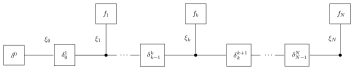
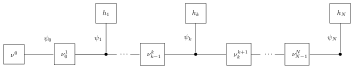
Fig. 1: Factor graph representation of posterior density (4)

The message updates in factor graph using max-product can be computed as follows

$$m_{f_{N}\rightarrow\xi_{N}} =f_{N},\quad m_{\xi_{N}\rightarrow\delta_{N-1}^{N}}=f_{N}$$

$$m_{\delta_{N-1}^{N}\rightarrow\xi_{N-1}} \propto\underset{\xi_{N}}{\max}~{}\delta_{N-1}^{N}\cdot m_{\xi_{N}\rightarrow\delta_{N-1}^{N}}$$

$$=\underset{\xi_{N}}{\max}~{}\frac{1}{\sqrt{2\pi\sigma^{2}}}\exp\left(\frac{-(\xi_{N}-\xi_{N-1})^{2}}{2\sigma^{2}}\right)$$

$$\cdot\exp\left(\lambda_{\xi}\xi_{N}\right)\mathbb{I}(U_{N}-\xi_{N})$$

which can be rearranged as

$$\begin{split}m_{\delta_{N-1}^{N}\rightarrow\xi_{N-1}}\propto\underset{\xi_{N}\leq U_{N}}{\max}~{}\exp&\big{(}A_{\xi,N}\xi_{N}^{2}+B_{\xi,N}\xi_{N-1}^{2}+\\ &C_{\xi,N}\xi_{N}\xi_{N-1}+D_{\xi,N}\xi_{N}\big{)}\end{split}$$ (6)

where

$$A_{\xi,N} \overset{\Delta}{=}-\frac{1}{2\sigma^{2}},\quad B_{\xi,N}\overset{\Delta}{=}-\frac{1}{2\sigma^{2}}$$

$$C_{\xi,N} \overset{\Delta}{=}\frac{1}{\sigma^{2}},\quad D_{\xi,N}\overset{\Delta}{=}\lambda_{\xi}\;.$$ (7)

Let $\bar{\xi}_{N}$ be the unconstrained maximizer of the exponent in the objective function above, i.e.,

$$\begin{split}\bar{\xi}_{N}=\arg\underset{\xi_{N}}{\max}~{}\big{(}&A_{\xi,N}\xi_{N}^{2}+B_{\xi,N}\xi_{N-1}^{2}+C_{\xi,N}\xi_{N}\xi_{N-1}+\\ &D_{\xi,N}\xi_{N}\big{)}\;.\\ \end{split}$$

This implies that

$$\bar{\xi}_{N}=-\frac{C_{\xi,N}\xi_{N-1}+D_{\xi,N}}{2A_{\xi,N}}\;.$$ (8)

If $\bar{\xi}_{N}>U_{N}$, then the estimation problem is solved, since $\hat{\xi}_{N}=U_{N}$. However, if $\bar{\xi}_{N}\leq U_{N}$, the solution is $\hat{\xi}_{N}=\bar{\xi}_{N}$. Therefore, in general, we can write

$$\hat{\xi}_{N}=\min\left(\bar{\xi}_{N},U_{N}\right)\;.$$

Notice that $\bar{\xi}_{N}$ depends on $\xi_{N-1}$, which is undetermined at this stage. Hence, we need to further traverse the chain backwards. Assuming that $\bar{\xi}_{N}\leq U_{N}$, $\bar{\xi}_{N}$ from (8) can be plugged back in (6) which after some simplification yields

$$\begin{split}m_{\delta_{N-1}^{N}\rightarrow\xi_{N-1}}\propto\exp\Bigg{\{}&\left(B_{\xi,N}-\frac{C_{\xi,N}^{2}}{4A_{\xi,N}}\right)\xi^{2}_{N-1}-\\ &\frac{C_{\xi,N}D_{\xi,N}}{2A_{\xi,N}}\xi_{N-1}\Bigg{\}}\;.\end{split}$$ (9)

Similarly the message from the factor $\delta_{N-2}^{N-1}$ to the variable node $\xi_{N-2}$ can be expressed as

$$m {}_{\delta_{N-2}^{N-1}\rightarrow\xi_{N-2}}\propto\underset{\xi_{N-1}\leq U_{N-1}}{\max}~{}\delta_{N-2}^{N-1}\cdot m_{\xi_{N-1}\rightarrow\delta_{N-2}^{N-1}}$$

$$= \underset{\xi_{N-1}}{\max}~{}\frac{1}{\sqrt{2\pi\sigma^{2}}}\exp\left(-\frac{(\xi_{N-1}-\xi_{N-2})^{2}}{2\sigma^{2}}\right)$$

$$\cdot\exp\left\{\left(B_{\xi,N}-\frac{C_{\xi,N}^{2}}{4A_{\xi,N}}\right)\xi^{2}_{N-1}-\frac{C_{\xi,N}D_{\xi,N}}{2A_{\xi,N}}\xi_{N-1}\right\}$$

$$\cdot\exp\left(\lambda_{\xi}\xi_{N-1}\right)\mathbb{I}(U_{N-1}-\xi_{N-1})\;.$$

The message above can be compactly represented as

$$m {}_{\delta_{N-2}^{N-1}\rightarrow\xi_{N-2}}\propto\underset{\xi_{N-1}\leq U_{N-1}}{\max}~{}\exp(A_{\xi,N-1}\xi_{N-1}^{2}+$$

$$B_{\xi,N-1}\xi_{N-2}^{2}+C_{\xi,N-1}\xi_{N-1}\xi_{N-2}+D_{\xi,N-1}\xi_{N-1})$$ (10)

where

$$A_{\xi,N-1} \overset{\Delta}{=}-\frac{1}{2\sigma^{2}}+B_{\xi,N}-\frac{C_{\xi,N}^{2}}{4A_{\xi,N}},\quad$$

$$B_{\xi,N-1} \overset{\Delta}{=}-\frac{1}{2\sigma^{2}},\quad C_{\xi,N-1}\overset{\Delta}{=}\frac{1}{\sigma^{2}}$$

$$D_{\xi,N-1} \overset{\Delta}{=}\lambda_{\xi}-\frac{C_{\xi,N}D_{\xi,N}}{2A_{\xi,N}}\;.$$

Proceeding as before, the unconstrained maximizer $\bar{\xi}_{N-1}$ of the objective function above is given by

$$\bar{\xi}_{N-1}=-\frac{C_{\xi,N-1}\xi_{N-2}+D_{\xi,N-1}}{2A_{\xi,N-1}}$$

and the solution to the maximization problem (10) is expressed as

$$\hat{\xi}_{N-1}=\min\left(\bar{\xi}_{N-1},U_{N-1}\right)\;.$$

Again, $\bar{\xi}_{N-1}$ depends on $\xi_{N-2}$ and therefore, the solution demands another traversal backwards on the factor graph representation in Fig. 1. By plugging $\bar{\xi}_{N-1}$ back in (10), it follows that

$$m_{\delta_{N-2}^{N-1}\rightarrow\xi_{N-2}}\propto$$

$$\exp\left\{\left(B_{\xi,N-1}-\frac{C_{\xi,N-1}^{2}}{4A_{\xi,N-1}}\right)\xi^{2}_{N-2}-\frac{C_{\xi,N-1}D_{\xi,N-1}}{2A_{\xi,N-1}}\xi_{N-2}\right\}$$ (11)

which has a form similar to (9). It is clear that one can keep traversing back in the graph yielding messages similar to (9) and (11). In general, for $i=1,\ldots,N-1$, we can write

$$\begin{split}A_{\xi,N-i}&\overset{\Delta}{=}-\frac{1}{2\sigma^{2}}+B_{\xi,N-i+1}-\frac{C_{\xi,N-i+1}^{2}}{4A_{\xi,N-i+1}}\\ B_{\xi,N-i}&\overset{\Delta}{=}-\frac{1}{2\sigma^{2}},\quad C_{\xi,N-i}\overset{\Delta}{=}\frac{1}{\sigma^{2}}\\ D_{\xi,N-i}&\overset{\Delta}{=}\lambda_{\xi}-\frac{C_{\xi,N-i+1}D_{\xi,N-i+1}}{2A_{\xi,N-i+1}}\end{split}$$ (12)

and

$$\bar{\xi}_{N-i} = -\frac{C_{\xi,N-i}\xi_{N-i-1}+D_{\xi,N-i}}{2A_{\xi,N-i}}$$ (13)

$$\hat{\xi}_{N-i} = \min\left(\bar{\xi}_{N-i},U_{N-i}\right)\;.$$ (14)

Using (13) and (14) with $i=N-1$, it follows that

$$\bar{\xi}_{1}=-\frac{C_{\xi,1}\xi_{0}+D_{\xi,1}}{2A_{\xi,1}},\quad\hat{\xi}_{1}=\min\left(\bar{\xi}_{1},U_{1}\right)\;.$$ (15)

Similarly, by observing the form of (9) and (11), it follows that

$$m_{\delta_{0}^{1}\rightarrow\xi_{0}}\propto\exp\left\{\left(B_{\xi,1}-\frac{C_{\xi,1}^{2}}{4A_{\xi,1}}\right)\xi^{2}_{0}-\frac{C_{\xi,1}D_{\xi,1}}{2A_{\xi,1}}\xi_{0}\right\}\;.$$ (16)

The estimate $\hat{\xi}_{0}$ can be obtained by maximizing (16).

$$\hat{\xi}_{0}=\bar{\xi}_{0}=\underset{\xi_{0}}{\max}~{}m_{\delta_{0}^{1}\rightarrow\xi_{0}}=\frac{C_{\xi,1}D_{\xi,1}}{4A_{\xi,1}B_{\xi,1}-C_{\xi,1}^{2}}\;.$$ (17)

The estimate in (17) can now be substituted in (15) to yield $\bar{\xi}_{1}$, which can then be used to solve for $\hat{\xi}_{1}$. Clearly, this chain of calculations can be continued using recursions (13) and (14).
Define

$$g_{\xi,k}(x)\overset{\Delta}{=}-\frac{C_{\xi,k}x+D_{\xi,k}}{2A_{\xi,k}}\;.$$ (18)

Lemma 1

For real numbers $a$ and $b$, the function $g_{\xi,k}(.)$ defined in (18) satisfies

$$g_{\xi,k}\left(\min(a,b)\right)=\min\left(g_{\xi,k}(a),g_{\xi,k}(b)\right)\;.$$

Proof: The constants $A_{\xi,k}$, $C_{\xi,k}$ and $D_{\xi,k}$ are defined in (7) and (12). The proof follows by noting that $\frac{-C_{\xi,k}}{2A_{\xi,k}}>0$ which implies that $g_{\xi,k}(.)$ is a monotonically increasing function.

Using the notation $g_{\xi,k}(.)$, it follows that

$$\bar{\xi}_{1} =g_{\xi,1}\left(\hat{\xi}_{0}\right),\quad\hat{\xi}_{1}=\min\left(U_{1},g_{\xi,1}\left(\hat{\xi}_{0}\right)\right)$$

$$\bar{\xi}_{2} =g_{\xi,2}\left(\hat{\xi}_{1}\right),\quad\hat{\xi}_{2}=\min\left(U_{2},g_{\xi,2}\left(\hat{\xi}_{1}\right)\right)$$

where

$$g_{\xi,2}\left(\hat{\xi}_{1}\right) =g_{\xi,2}\left(\min\left(U_{1},g_{\xi,1}\left(\hat{\xi}_{0}\right)\right)\right)$$

$$=\min\left(g_{\xi,2}\left(U_{1}\right),g_{\xi,2}\left(g_{\xi,1}\left(\hat{\xi}_{0}\right)\right)\right)$$ (19)

where (19) follows from Lemma 1. The estimate $\hat{\xi}_{2}$ can be expressed as

$$\hat{\xi}_{2} =\min\left(U_{2},\min\left(g_{\xi,2}\left(U_{1}\right),g_{\xi,2}\left(g_{\xi,1}\left(\hat{\xi}_{0}\right)\right)\right)\right)$$

$$=\min\left(U_{2},g_{\xi,2}\left(U_{1}\right),g_{\xi,2}\left(g_{\xi,1}\left(\hat{\xi}_{0}\right)\right)\right)\;.$$

Hence, one can keep estimating $\hat{\xi}_{k}$ at each stage using this strategy. Note that the estimator only depends on functions of data and can be readily evaluated. For $m\geq k$, define

$$G_{\xi,k}^{m}(.)\overset{\Delta}{=}g_{\xi,m}\left(g_{\xi,m-1}\ldots g_{\xi,k}\left(.\right)\right)\;.$$ (20)

The estimate $\hat{\xi}_{N}$ can, therefore, be compactly represented as

$$\hat{\xi}_{N}=\min\left(U_{N},G_{\xi,N}^{N}\left(U_{N-1}\right),\dots,G_{\xi,2}^{N}\left(U_{1}\right),G_{\xi,1}^{N}\left(\hat{\xi}_{0}\right)\right)\;.$$ (21)

By a similar reasoning, the estimate $\hat{\psi}_{N}$ can be analogously expressed as

$$\hat{\psi}_{N}=\min\left(V_{N},G_{\psi,N}^{N}\left(V_{N-1}\right),\dots,G_{\xi,2}^{N}\left(V_{1}\right),G_{\xi,1}^{N}\left(\hat{\psi}_{0}\right)\right)$$

and the factor graph based clock offset estimate (FGE) $\hat{\theta}_{N}$ is given by

$$\hat{\theta}_{N}=\frac{\hat{\xi}_{N}-\hat{\psi}_{N}}{2}\;.$$ (22)

It only remains to calculate the functions of data $G(.)$ in the expressions for $\hat{\xi}_{N}$ and $\hat{\psi}_{N}$ to determine the FGE estimate $\hat{\theta}_{N}$. With the constants defined in (7), it follows that

$$G_{\xi,N}^{N}(U_{N-1})=-\frac{C_{\xi,N}U_{N-1}+D_{\xi,N}}{2A_{\xi,N}}=U_{N-1}+\lambda_{\xi}\sigma^{2}\;.$$

Similarly it can be shown that

$$G_{\xi,N-1}^{N}(U_{N-2})=U_{N-2}+2\lambda_{\xi}\sigma^{2}$$

and so on. Using the constants defined in (12) for $i=N-1$, it can be shown that $\hat{\xi}_{0}=\frac{C_{\xi,1}D_{\xi,1}}{4A_{\xi,1}B_{\xi,1}-C_{\xi,1}^{2}}=+\infty$. This implies that $G_{\xi,1}^{N}(\hat{\xi}_{0})=+\infty$. Plugging this in (21) yields

$$\hat{\xi}_{N}=\min(U_{N},U_{N-1}+\lambda_{\xi}\sigma^{2},\ldots,U_{1}+(N-1)\lambda_{\xi}\sigma^{2})\;.$$

Similarly, the estimate $\hat{\psi}_{N}$ is given by

$$\hat{\psi}_{N}=\min(V_{N},V_{N-1}+\lambda_{\psi}\sigma^{2},\ldots,V_{1}+(N-1)\lambda_{\psi}\sigma^{2})\;$$

and the estimate $\hat{\theta}_{N}$ can be obtained using (22) as

$$\hat{\theta}_{N}=\frac{1}{2}\min(U_{N},U_{N-1} +\lambda_{\xi}\sigma^{2},U_{N-2}+2\lambda_{\xi}\sigma^{2},$$

$$\ldots,U_{1}+(N-1)\lambda_{\xi}\sigma^{2})-$$

$$\frac{1}{2}\min(V_{N},V_{N-1} +\lambda_{\psi}\sigma^{2},V_{N-2}+2\lambda_{\psi}\sigma^{2},$$

$$\ldots,V_{1}+(N-1)\lambda_{\psi}\sigma^{2})\;.$$ (23)

As the Gauss-Markov system noise $\sigma^{2}\rightarrow 0$, (23) yields

$$\hat{\theta}_{N}\rightarrow\hat{\theta}_{\textrm{ML}}=\frac{\min\left(U_{N},\ldots,U_{1}\right)-\min\left(V_{N},\ldots,V_{1}\right)}{2}$$ (24)

which is the ML estimator proposed in [6].

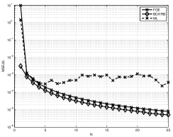
Fig. 2: Comparison of MSE of $\hat{\theta}_{N}$ and $\hat{\theta}_{\textrm{ML}}$.

4 Simulation Results

With $\lambda_{\xi}=\lambda_{\psi}=10$ and $\sigma=10^{-2}$, Fig. 2 shows the MSE performance of $\hat{\theta}_{N}$ and $\hat{\theta}_{\textrm{ML}}$, compared with the Bayesian Chapman-Robbins bound (BCHRB). It is clear that $\hat{\theta}_{N}$ exhibits a better performance than $\hat{\theta}_{\textrm{ML}}$ by incorporating the effects of time variations in clock offset. As the variance of the Gauss-Markov model accumulates with the addition of more samples, the MSE of $\hat{\theta}_{\textrm{ML}}$ gets worse. Fig. 3 depicts the MSE of $\hat{\theta}_{N}$ in (23) with $N=25$. The horizontal line represents the MSE of the ML estimator (24). It can be observed that the MSE obtained by using the FGE for estimating $\theta$ approaches the MSE of the ML as $\sigma<10^{-3}$.

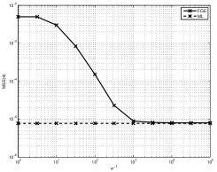
Fig. 3: MSE in estimation of $\theta_{N}$ vs $\sigma$.

5 Conclusion

The estimation of a possibly time-varying clock offset is studied using factor graphs. A closed form solution to the clock offset estimation problem is presented using a novel message passing strategy based on the max-product algorithm. This estimator shows a performance superior to the ML estimator proposed in [6] by capturing the effects of time variations in the clock offset efficiently.