Kernel PCA for type Ia supernovae photometric classification

Abstract

The problem of supernova photometric identification will be extremely important for large surveys in the next decade. In this work, we propose the use of Kernel Principal Component Analysis (KPCA) combined with k = 1 nearest neighbour algorithm (1NN) as a framework for supernovae (SNe) photometric classification. The method does not rely on information about redshift or local environmental variables, so it is less sensitive to bias than its template fitting counterparts. The classification is entirely based on information within the spectroscopic confirmed sample and each new light curve is classified one at a time. This allows us to update the principal component (PC) parameter space if a new spectroscopic light curve is available while also avoids the need of re-determining it for each individual new classification. We applied the method to different instances of the Supernova Photometric Classification Challenge (SNPCC) data set. Our method provide good purity results in all data sample analysed, when SNR$\geq$5. As a consequence, we can state that if a sample as the post-SNPCC was available today, we would be able to classify $\approx 15\%$ of the initial data set with purity $\gtrsim$ 90% (D₇+SNR3). Results from the original SNPCC sample, reported as a function of redshift, show that our method provides high purity (up to $\approx 97\%$), specially in the range of $0.2\leq z<0.4$, when compared to results from the SNPCC, while maintaining a moderate figure of merit ($\approx 0.25$). This makes our algorithm ideal for a first approach to an unlabelled data set or to be used as a complement in increasing the training sample for other algorithms. We also present results for SNe photometric classification using only pre-maximum epochs, obtaining 63% purity and 77% successful classification rates (SNR$\geq$5). In a tougher scenario, considering only SNe with MLCS2k2 fit probability $>$0.1, we demonstrate that KPCA+1NN is able to improve the classification results up to $>95\%$ (SNR$\geq$3) purity without the need of redshift information. Results are sensitive to the information contained in each light curve, as a consequence, higher quality data points lead to higher successful classification rates. The method is flexible enough to be applied to other astrophysical transients, as long as a training and a test sample are provided.

1 Introduction

Since its discovery (Riess et al., 1998; Perlmutter et al., 1999), dark energy (DE) has become a big challenge in theoretical physics and cosmology. In order to improve our understanding about its nature, multiple observations are used to add better constraints over DE characteristics (e.g., Mantz et al., 2010; Blake et al., 2011; Plionis et al., 2011). In special, large samples of type Ia supernovae (SNe Ia) are being used to measure luminosity distances as a function of redshift in order to constraint cosmological parameters (e.g., Kessler et al., 2009; Ishida & de Souza, 2011; Benitez-Herrera et al., 2012; Conley et al., 2011). As part of the efforts towards understanding DE, we expect many thousands of SNe candidates from large photometric surveys, such as the Large Synoptic Survey Telescope (LSST) (Tyson, 2002), SkyMapper (Schmidt et al., 2005) and the Dark Energy Survey (DES) (Wester & Dark Energy Survey Collaboration, 2005). However, with rapidly increasing available data, it is already impracticable to provide spectroscopical confirmation for all potential SNe Ia discovered in large field imaging surveys. After a great effort in allocating their resources for spectroscopic follow-up, the SuperNova Legacy Survey (SNLS)(Astier et al., 2006) and the Sloan Digital Sky Survey (SDSS)(York et al., 2000), were able to provide confirmation for almost half of their light-curves. These constitute the major SNe Ia samples currently available, but it is very unlikely that their power of spectroscopic follow-up will continue to increase as it did in the last decade (Kessler et al., 2010). In this context, we do not have much choice left other than develop (or adapt) statistical and computational tools which allow us to perform classification on photometric data alone. Beyond that, such tools should ideally provide a quick and flexible framework, where information from new data may be smoothly added in the pipeline.

Trying to solve this puzzle, in the recent years a good diversity of techniques were applied to the problem of SNe photometric classification (Poznanski et al., 2002; Johnson & Crotts, 2006; Sullivan et al., 2006; Poznanski et al., 2007; Kuznetsova & Connolly, 2007; Kunz et al., 2007; Sako et al., 2008; Rodney & Tonry, 2009; Gong et al., 2010; Falck et al., 2010). Most of them use the idea of template fitting, so the classification is estimated by comparison between the unlabelled SN and a set of confirmed light curve templates. The method starts with the hypothesis that the new, unlabelled, light curve belongs to one of the categories in the template sample. The procedure then continues to determine which category best resembles the characteristic of this new object. It produced good results (Sako et al., 2008), but its final classification rates are highly sensitive to the characteristics of the template sample.

To overcome such difficulty, Newling et al. (2011); Sako et al. (2011) describe different techniques which address a posterior probability to each classification output. These algorithms produce not a specific type for each SN, but a probability of belonging to each one of the template classes. Such an improvement allow the user to impose selection cuts on posterior probability and, for example, use for cosmology only those SNe with a high probability of being Ia.

Another interesting approach proposed by Kunz et al. (2007), and further developed by Newling et al. (2012), takes a somewhat different path. Instead of separating between Ia and non-Ia before the cosmological analysis, they use all the available data. However, the influence of each data point in determining the cosmological parameters is weighted according to their posterior probability (obtained from some classifier like that of Sako et al. (2011), for example). The method was able to identify the fiducial cosmological parameters in a simulated data set, although some bias still remains and worth further investigation.

Following a different line of thought, Richards et al. (2012) (hereafter R2012) proposes the use of diffusion maps to translate each light curve into a low dimensional parameter space. Such space is constructed using the entire sample and, after a suitable representation is found, the label of the spectroscopic sample is revealed. In the final step a random forest classification algorithm is used to assign a label to the photometric light curves, based on their low dimensional distribution when compared to the one from the spectroscopically confirmed SNe. Results were comparable to template fitting methods in a simulated data set, but it also showed large sensitivity to the representativeness between training and test samples.

More recently, Karpenka et al. (2012) presented a two-step algorithm where each light curve in the spectroscopic sample is first fitted to a parametric function. The values of parameters found are subsequently used in training a neural network (NN) algorithm. The NN is then applied to the photometric sample and, for each light curve, it returns the probability of being a Ia. Their classification results are overall not depending on redshift distribution and, as other analysis cited before, can be vary significantly depending on the training sample used.

In order to better understand and compare the state of art of photometric classification techniques, Kessler et al. (2010) released the SuperNova Photometric Classification Challenge (hereafter, SNPCC). It consisted of a blind sample of $\sim$20.000 SNe light curves, generated using the SuperNova ANAlysis (SNANA) light curve simulator (Kessler et al., 2009), and designed to mimic data from the DES. Approximately 1000 of these were given with labels, so to represent a spectroscopically confirmed sub-sample. The participants were offered 2 instances of the data, with and without the host galaxy photometric redshift (photo-z). Around a dozen entries were submitted to the Challenge and, although none of them obtained an outstanding result when compared to others, it provided a clear picture of what can be done currently and what we should require from future surveys in order to improve photometric classifications. There was also an instance of the data containing only observations before maximum, which aimed at choosing potential spectroscopic follow-up candidates. However, this data set did not received replies from the participants (Kessler et al., 2010). After the Challenge, the organizers released an updated version of the data, including all labels, bug fixes and other improvements found necessary during the competition. The works of Newling et al. (2011), R2012 and Karpenka et al. (2012) present detailed results from applying their algorithm to this post-SNPCC data.

Given the stimulating activity in the field of SNe photometric classification, and the urgency with which the problem imposes itself, our purpose here is to present an alternative method which optimizes purity in the final SNe Ia sample, in order to provide a statistically significant number of photometrically classified SNe Ia for cosmological analysis. Our algorithm uses a machine learning approach, similar in philosophy to the entry of R2012 submitted to the SNPCC. This class of statistical tools has already been applied to a variety of astronomical topics (for a recent review see Ball & Brunner (2010)).

We propose the use of Kernel Principal Component Analysis (hereafter, KPCA) as a tool to find a suitable low dimension representation of SNe light curves. In constructing this low dimensional space only the spectroscopically confirmed sample is used. Each unlabelled light curve is then projected into this space one at a time and a k-nearest neighbour (kNN) algorithm performs the classification. The procedure was applied to the post-SNPCC data set using the entire light curves and also using only pre-maximum observations. In order to allow a more direct comparison with SNPCC results, we also applied the algorithm to the complete light curves in the original SNPCC data set.

Our procedure returns purity levels higher than to top ranked methods reported in the SNPCC. The results are sensitive to the spectroscopic sample, but more on the quality of each individual observation than on representativeness between spectroscopic and photometric samples. Assuming that results can only be as good as the input data, we perform classification in sub-samples of SNPCC and post-SNPCC data based on signal to noise ratio (SNR) levels.

Considering only light curves with Multi-color Light Curve Shape (MLCS2k2) (Jha et al., 2007) fit probability, FitProb$>$0.1, we demonstrate that our method is capable of increasing purity and successful classification rates even in a context with only light curves very similar between each other.

The paper is organized as follows: section 2 briefly describe linear PCA and its transition to the KPCA formalism. In section 3 we detailed the cross-validation and kNN algorithm used for classification. In section 4 we present the guidelines to prepare the raw light curve data into a data vector suitable for KPCA. The results applied to a best case scenario simulation, to the post-SNPCC data and comparison with MLCS2k2 fit probability results are shown in section 5. We report outcomes from applying our method to the original SNPCC data set in section 6. Finally, we discuss the results and future perspectives in section 7. Throughout the text, mainly in section 2, we refer to a few theorems and mathematical statements are made. Those which are most crucial for the development of the KPCA argument are briefly demonstrated in appendix A. A detailed description of results achieve using linear PCA+kNN algorithm is presented in appendix B. Appendix C shows classification rates as a function of redshift and SNR cuts and appendix D displays our achievements when no SNR cuts are applied. Graphical representation of results from SNPCC data set for all the tests we performed, which can be directly compared to those of Kessler et al. (2010) are displayed in appendix E. Complete summary tables reporting the number of data points in different sub-samples of SNPCC and post-SNPCC data and classification results mentioned in the text are shown in appendix F.

2 Principal Component Analysis

The main goal of PCA is to reduce an initial large number of variables to a smaller set of uncorrelated ones, called Principal Components (PCs). This set of PCs is capable of reproducing as much variance from the original variables as possible. Each of them can be viewed as a composite variable summarizing the original ones, and its eigenvalue indicates how successful this summary is. If all variables are highly correlated, one single PC is sufficient to describe the data. If the variables form two or more sets, and correlations are high within sets and low between sets, a second or third PC is needed to summarize the initial variables. PCA solutions with more than one PC are referred to as multi-dimensional solutions. In such cases, the PCs are ordered according to their eigenvalues. The first component is associated with the largest eigenvalue, and accounts for most of the variance, the second accounts for as much as possible of the remaining variance, and so on.

There are a few different ways which lead to the determination of PCs. Particularly, we have already shown that it is possible to derive the PCs beginning from a theoretical description of the likelihood function (e.g., Ishida & de Souza, 2011; Ishida et al., 2011).

In the present work we are interested in exploring the KPCA and, as a consequence, our description shall be based on dot products. In doing so, the connection between PCA and KPCA occurs almost smoothly. We follow closely Hofmann et al. (2008) and Max Welling’s notes A first encounter with Machine Learning, which the reader is refereed to for a more complete mathematical description of the steps shown here.

2.1 Linear PCA

We begin by defining a set of $N$ vectors $G=\{\mathbf{g_{1},\mathbf{g_{2}},...,\mathbf{g_{N}}}\}$, which contains our observational measurements. If $\mathbf{g_{\rm mean}}$ is the vector of mean values of $G$, let $X\in\mathbb{R}^{n}$ be the set of vectors which holds the centered observations,

$$\mathbf{x}_{k}=\mathbf{g_{k}}-\mathbf{g_{\rm mean}}.$$ (1)

In order to find the PCs, we shall diagonalize the covariance matrix

$$C=\frac{1}{N}\sum_{i=1}^{N}\mathbf{x}_{i}\mathbf{x}_{i}^{T}.$$ (2)

This can be accomplished by solving the eigenvalue equation

$$\lambda_{i}\mathbf{v}_{i}=C\mathbf{v}_{i},$$ (3)

where $\lambda_{i}>0$ are the eigenvalues and $\mathbf{v}_{i}\in\mathbb{R}^{n}$ the eigenvectors of the covariance matrix.

If we consider $V$ the set of eigenvectors of $C$ and $P$ the set of data points projections in $V$, the elements of $P$ will be given by

$$\mathbf{p_{i}}=A_{l}^{T}\mathbf{x}_{i},$$ (4)

where $A_{l}$ is the matrix formed by the $l$ first PCs as columns. It is possible to show that the elements of $P$ will be uncorrelated, independently of the dimension chosen for matrix $A_{l}$.

This is where the dimensionality reduction takes place. We can choose the number of PCs that will compose the matrix $A_{l}$ based on how much of the initial variance we are willing to reproduce in $P$. At the same time, depending on the nature of our data, the spread of the points in the PCs space might also reveal some underlying information, as the existence of two classes of data points, for example.

The main goal of this work is to use PCA to project the data in a sub-space where photometric data vectors associated with different supernova types can be separated. In order to do so, our first step is to show that it is possible to calculate the projected data points $\in P$ without the need of explicitly defining the eigenvectors $\in V$. This will be important when we consider non-linear correlations in the next sub-section.

Given that all vectors $\in V$ must lie in the space spanned by the data vectors $\in X$, we can show that (see appendix A)

$$\mathbf{v}_{a}=\sum_{i=1}^{N}\alpha_{i}^{a}\mathbf{x}_{i},\qquad{\rm with}\qquad\alpha_{i}^{a}=\frac{\mathbf{x}_{i}^{T}\mathbf{v}_{a}}{N\lambda_{a}},$$ (5)

and as a consequence, instead of solving equation (3) we can also find the elements of $P$ by solving the projected equations

$$\mathbf{x}_{i}^{T}C\mathbf{v}_{a}=\lambda_{a}\mathbf{x}_{i}^{T}\mathbf{v}_{a},\quad\forall i,a.$$ (6)

This leads us to an eigenvalue equation in the form

$$K\mathbf{\alpha}^{a}=\tilde{\lambda_{a}}\mathbf{\alpha}^{a},$$ (7)

where

$$K_{ij}=\mathbf{x}_{i}^{T}\mathbf{x}_{j},$$ (8)

and $\tilde{\lambda_{a}}=N\lambda_{a}$. Normalizing $\mathbf{v}_{a}$, we can also show that $||\alpha^{a}||=1/\sqrt{N\lambda_{a}}$.

Finally, consider a test data vector $\mathbf{n}$. Its projections in the PCs space are given by

$$\mathbf{v}_{a}^{T}\mathbf{n}=\sum_{i=1}^{N}\alpha_{i}^{a}\mathbf{x}_{i}^{T}\mathbf{n}=\sum_{i=1}^{N}\alpha_{i}^{a}K(\mathbf{x}_{i},\mathbf{n}),$$ (9)

where $K(\mathbf{x}_{i},\mathbf{n})=\mathbf{x}_{i}^{T}\mathbf{n}$.

This demonstration was specifically designed to rely only on the matrix $K$. Although, the classification we aim in this work is not possible in the linear regime. In order to be able to disentangle light curves from different supernovae, we need to perform PCA in a higher dimensional space, where the characteristics we are interested in are linearly correlated.

2.2 Kernel Principal Component Analysis

KPCA generalizes PCA by first mapping the data non-linearly into a higher dimensional dot product space $\mathbb{F}$ (hereafter, feature space):

$$\Phi:\mathbb{R}^{n} \rightarrow \mathbb{F}$$

$$\mathbf{x} \rightarrow \Phi(\mathbf{x}),$$ (10)

where $\Phi$ is a nonlinear function and $\mathbb{F}$ has arbitrary (usually very large) dimensionality.

The covariance matrix, $C_{\rm F}\in\mathbb{F}$, will be defined similarly as

$$C_{\rm F}=\frac{1}{N}\sum_{i=1}^{N}\Phi(x_{i})\Phi(x_{i})^{T}.$$ (11)

We assume that $\Phi(\mathbf{x}_{i})$ are centred in feature space. We shall come back to this point latter on.

Consider $\mathbf{v}_{\Phi}^{l}$ the $l-th$ eigenvector of $C_{\rm F}$ and $\lambda_{\Phi}^{l}$ its $l-th$ eigenvalue. Using the same line of argument shown in the previous subsection, we can define an kernel $N\times N$ matrix

$$K_{F}(\mathbf{x}_{i},\mathbf{x}_{j})=(\Phi(\mathbf{x}_{i})\cdot\Phi(\mathbf{x}_{j})),$$ (12)

which allows us to compute the value of dot product in $\mathbb{F}$ without having to carry out the map $\Phi$. The kernel function has to satisfy the Mercer’s theorem to ensure that it is possible to construct a mapping into a space where $K_{\rm F}$ acts as a dot product. The projection of a new test point, $\mathbf{n}$, is given by

$$(\mathbf{v}_{\Phi}^{l}\cdot\Phi(\mathbf{n}))=\sum_{i=1}^{N}\alpha_{\Phi_{i}}^{l}K_{F}(\mathbf{x_{i}},\mathbf{n}),$$ (13)

where $\alpha_{\Phi_{i}}^{l}$ is defined by the solutions to the eigenvalue equation $N\lambda_{\Phi}\alpha_{\Phi}=K_{F}\alpha_{\Phi}$.

Finally, it is important to stress that all the arguments shown in this sub-section rely on the assumption that the data are centred in feature space. This is not a direct consequence of using $X$ instead of $G$. Equation (1) is responsible for centring data vectors in $\mathbb{R}^{n}$, in order to perform centralization in $\mathbb{F}$, we need to construct the kernel matrix using $\Phi(\boldsymbol{x})-\widetilde{\Phi(\boldsymbol{x})}$. This can also be computed without any information about the function $\Phi$. It is shown in appendix A that the centred kernel matrix, $\widetilde{K_{F}}$, can be expressed in terms of the non-centered kernel matrix, $K_{F}$, as

$$\widetilde{K_{F}}=K_{F}-1_{N}K_{F}-K_{F}1_{N}+1_{M}K_{F}1_{N},$$ (14)

where $(1_{N})_{ij}=1/N$. The reader should be aware that we always refer to the centred kernel matrix $\widetilde{K_{F}}$. However, for the sake of simplicity, the tilde is not used in our notation.

At this point, we have the tools necessary to compute the centred kernel matrix based on dot products in input space. However, we still need to choose a form for the kernel function $k(\mathbf{x}_{i},\mathbf{x}_{j}):=K_{{F}_{ij}}$.

In the present work, for the sake of simplicity, we make an a priori choice of using a Gaussian kernel,

$$k(\mathbf{x}_{i},\mathbf{x}_{j})=\exp\left[-\frac{\|\mathbf{x}_{i}-\mathbf{x}_{j}\|^{2}}{2\sigma^{2}}\right],$$ (15)

where the value of $\sigma$ is determined by a cross-validation processes (see subsection 3.2). Although, it is important to emphasize that there is extensive literature on how to choose the appropriate kernel for each particular data set at hand (Lanckriet et al., 2004; Zang et al., 2006). To compare the analysis between different kernel choices is out of the scope of this work. As our goal is to focus on the KPCA procedure itself, we are using the standard kernel choice. An analysis of performances from different kernel choices within the KPCA framework should certain be topic of future research.

3 Classification

By virtue of what was presented so far, we have a set of centred data points, $X$, and a kernel function, $k(\mathbf{x}_{i},\mathbf{x}_{j})$. This allows us to calculate the kernel matrix in feature space, $K_{F}$, and its corresponding eigenvalues, $\boldsymbol{\alpha}_{\Phi}$. Using equation (9), we can obtain the projection of each data point in the eigenvectors of $C_{\rm F}$.

From now on, we will work in the space spanned by these eigenvectors. More precisely, we will look for a 2-dimensional sub-space of $\mathbf{v}_{\Phi}$, which can optimize our ability to separate the projected data in 2 different classes (namely Ia and non-Ia supernovae). We chose to keep this sub-space bi-dimensional in order to avoid over-fitting to the particular data set we are analysing.

The procedure describe before is now applied to two different instances of our data. A data set suitable for the analysis we present here must be composed of two sub-samples. For one of them we have the appropriate label for each data point (we know which class they belong to), from now on this sub-set will be called training sample. For the other sub-sample (hereafter test sample) the labels are not available, and we want to classify them based on our previous knowledge about the training sample.

In a first moment, we will concentrate our efforts in the training sample. Its projections in a certain pair of PCs are calculated through equation (9). Given that labels of data in this sample are known, we can calculate projections in different PCs and determine which PC pair better translates the initial light curves into a separable point configuration.

3.1 The k-Nearest Neighbor algorithm

Our choice of which subspace of $\mathbf{v}_{\Phi}$ is more adequate for a specific data situation will be balanced by how well we can classify the training sample using the k-Nearest Neighbor algorithm (kNN).

kNN is one of the most simple classification algorithms and it has been proved efficient in low dimension parameter spaces, ($\rm{dim}\leq 10$, for a further discussion on kNN performance in higher dimensions see Beyer et al. (1999)). The method begins with the training sample organized as $q_{i}=(x_{i},y_{i})$, where $x_{i}$ is the $i-th$ data vector and $y_{i}$ its label, and a definition of distance between 2 data vectors $d(x_{i},x_{j})$. Given a new unlabelled test point $q_{t}(x_{t},)$, the algorithm computes the distance between $x_{t}$ and all the other points in the training sample, $d(x_{t},\mathbf{x})$, ordering them from lower to higher distance. The labels of the first $k$ data vectors (the ones closer to $x_{t}$) are counted as votes in the definition of $y_{t}$. Finally, $y_{t}$ is set as the label with highest number of votes. Given this last voting characteristic, kNN is many times refereed to as a type of majority vote classifier (James, 1998).

Throughout our analysis, we used an Euclidean distance metric and order $k=1$. As this is the first attempt in applying KPCA to the photometric problem, we chose to be bounded by the Bayes error rate (hereafter, BER). The BER is defined as the error rate resulting from the best possible classifier. It can be shown that, in the limit of large samples, the error rate of a $k=1$ nearest neighbour algorithm is never larger than $2\times$ BER (for a scratch of the proof see Ripley (1996), page 195). From now on, this will be refereed to as 1NN algorithm (nearest neighbour with $k=1$).

So far we described how to define a convenient 2-dimensional space where our data points will be separated in Ia and non-Ia populations (sub-section 2.2) and a classification tool that allows us to add a label to a new, unlabelled data point (subsection 3.1). However, we still need to define which pair of PCs of the feature space better maps our data. This is done in the next sub-section.

3.2 Cross-validation

The main idea behind the cross-validation procedure is to remove from the training sample a random set of $M$ data points, $T^{\rm{out}}$. The remaining part of the training sample is given as input in some classifier algorithm and used to classify the points in $T^{\rm{out}}$. In this way, we can measure the success rate of the classifier over different random choices of $T^{\rm{out}}$ and also compare results from different classifiers given the same training and $T^{\rm{out}}$ sets (for a complete review on cross-validation methods see Arlot & Celisse (2010)).

The the number of points in $T^{\rm{out}}$ is a free parameter and must be defined based on the clustering characteristics of the given data set. Here we chose the most classical exhaustive data splitting procedure, sometimes called Leave One Out (LOO) algorithm. As the name states, we construct $N$ sub-samples $T^{\rm{out}}$, each one containing only one data point, $M=1$. The training sample is then cross-validated and the performance judged by the average number of correct classifications.

Data exhaustive algorithms like LOO have a larger variance in the final results, although, they are highly recommended for avoiding biases regarding local data clustering and some non-uniform geometrical distribution of data points in a given parameter space.

3.2.1 The algorithm

In the context of KPCA, we used LOO and 1NN algorithms to decide the appropriate pair of PCs and value of $\sigma$ (equation (15)) for each data set.

Figure 1: Normalized light curves from SIM1. Left: SNe Ia light curve. The plot shows the flux measurements (blue dots) and fitted spline function (red curve), normalized as explained in the text. Right: Example of normalized light curves functions for Ia (red thick), Ib (green dashed), Ibc (orange short-dashed), Ic (cyan dashed), IIL (blue thin), IIn (brown short-dashed) and IIP (purple dot-dashed), according to SNANA classification. The panels from top to bottom run over the DES filters $\{g,r,i,z\}$. The horizontal axis is in units of days since maximum brightness in $r$ band.

The next trick question to answer is: which PCs we should test with the algorithms described before? Obviously there is a high number of vectors in $\mathbf{v}_{\Phi}$ and it would not be possible to test all available pairs. Fortunately, we can make use of the fact that the firsts eigenvectors $\mathbf{v}_{\Phi}$ (those with larger eigenvalues) represent directions of greater data variance in feature space. Although we cannot visualize such vectors, it is easy to confirm that the magnitude of data points projections in $\mathbf{v}_{\Phi}^{l}$ become very similar to each other for higher $l$. In other words, the smaller eigenvalues correspond to PCs carrying mostly noise, so their projections will, in average, be very similar, and meaningless (Schölkopf et al., 1996). For classification purposes, one expects that the PC pair tailored to provide geometrical separation of the data projection into classes will be among the PCs with higher eigenvalues.

For the case studied here, we restrict ourselves to testing the first 5 PCs in a first round and extend the search to other PCs only if the classification success rate do not monotonically decrease with the use of higher PCs. In the same line of thought, we start our search with $\sigma\in\{0.1,2.0\}$ in a grid with steps of 0.1 and make this interval wider only if the results do not converge after a first round of evaluations.

The cross-validation algorithm we used is better summarized as:

1. Pick a PC pair, $\{\rm{PC}_{\rm{A}},\rm{PC}_{\rm{B}}\}$.

2. Define a grid of values for parameter $\sigma$, $\sigma\in\{\sigma_{\rm{min}},\sigma_{\rm{max}}\}$.

3. Pick a value from the above grid, $\sigma_{\rm test}$.

4. Cross validate the training sample using the KCPA projections in the chosen PCs, 1NN and LOO algorithms.

5. Calculate the average classification success rate for $\{\sigma_{\rm test},{\rm PC}_{\rm A},{\rm PC}_{\rm B}\}$.

6. Repeat steps (ii) to (v) 10 times. If the average number of successful classifications monotonically decreases in the upper and lower boundaries of $\sigma$, go to step (vii). If not, repeat steps (ii) to (vi) until they do.

7. Repeat steps (i) to (vi) for all pairs of $\{{\rm A},{\rm B}\}\in\{1,5\}$.

8. If the average number of successful classifications monotonically decreases when using higher PCs, go to step (ix). Otherwise, consider $\{{\rm A},{\rm B}\}\in\{1,10\}$ and repeat steps (i) to (viii).

9. Choose for $\{\sigma,{\rm PC}_{\rm A},{\rm PC}_{\rm B}\}$, values corresponding to the largest average number of successful classifications.

Once the cross-validation is completed, we use the resulting parameter values to calculate the training sample projections in PC space. We can finally use 1NN algorithm to assign a label to each data point in the test sample. The final procedure of classifying the test sample is called KPCA+1NN algorithm throughout the text.

The framework described so far can be applied to any set of astrophysical objects, as long as we have a training and a test sample. The cross-validation procedure is performed only in the training sample and each point in the test sample is classified at a time. This avoids running the whole machinery again every time one new point is added to the test sample, and prevent us from introducing misleading data as part of the features to be mapped by the PCs. However, the parameter space composed by the PC pair and value of $\sigma$ can always be updated if we have at hand new data points whose types are known. Only then it is necessary to re-run the cross-validation process.

From now on we focus on the problem of photometrically classifying SNe Ia as a practical example, although the exact same steps could be applied for any transient with observable light curves. In the next section, we describe how the light curve data should be prepare before we try to classify them.

Table 1: Description of the light curve selection cuts. The SNe were required at least one observation in $t\leq t_{\rm low}$, one in $t\geq t_{\rm up}$ and at least 3 observations satisfying a given SNR requirement in each filter in order to be included in any of the data sets analysed in this work. These selection cuts were applied for training and test samples within a specific data set.

	$t_{\rm low}$	$t_{\rm up}$	$\Delta$
$D_{1}$	-3	+24	1
$D_{2}$			3
$D_{3}$	0	+15	1
$D_{4}$			3
$D_{5}$	-10	0	1
$D_{6}$			3
$D_{7}$	-3	+45	1
$D_{8}$			3

4 Light curve preparation

In case we have b different filters, the observational data available from the $l-th$ SN can be arranged as $\mathbf{F}^{l}=\{F^{l}_{1},...,F^{l}_{b}\}$. Considering the $i-th$ filter, $\left(\mathbf{F}^{l}\right)_{i}=\{\{t^{l}_{i1},F^{l}_{i1},\sigma^{l}_{{\rm F}i1}\},...,\{t^{l}_{ie},F^{l}_{ie},\sigma^{l}_{{\rm F}ie}\}\}$. In our notation, the $t^{l}_{ij}$ correspond to the $j-th$ observation epoch (in MJD), $F^{l}_{ij}$ is the measured flux at $t^{l}_{ij}$, $\sigma^{l}_{{\rm F}ij}$ is the error in flux measurement and $e$ is the total number of observation epochs in filter $i$.

Our next task is to translate the time of each observation from MJD to the time since maximum brightness in a particular filter. Which filter shall be used as a reference does not have much influence in the final result. The ideal is to choose a band where the ability to determine the time of peak brightness is greater, and use that reference band for all SN in the sample. The time of maximum brightness in our reference band for the $l-th$ SN is addressed as $t^{l}_{\rm max}$. As a result, we obtain data points in a particular filter $i$ as $F^{l}_{i}=\{\{\left(t_{\rm max}^{l}\right)_{i1},F^{l}_{i1},\sigma^{l}_{i\rm F1}\},...,\{\left(t_{\rm max}^{l}\right)_{ie},F^{l}_{ie},\sigma^{l}_{i\rm Fe}\}\}$, where $\left(t_{\rm max}^{l}\right)_{ij}=t^{l}_{ij}-t^{l}_{\rm max}$.

Figure 2: Classification results from SIM1. Blue circles (Ia) and purple squares (non-Ia) represent the geometrical locus defined by the training sample. Top: Red dots correspond to SNe Ia in the test sample. Bottom: Cyan dots correspond to non-Ia SNe in the test sample. The plot also shows calculated values for eff_A and pur.

We must also deal with the fact that, in a real situation, the input from observations consists in some non-uniform sampling of the light curve in various (most cases more than 3) different filters for each SNe. Although, it is necessary to translate such information into a grid equally spaced in time. This is done by using a cubic regression spline fit for each light curve. The spline fit was chosen based on its ability to fit non-uniform functions in a parameter independent manner. As a consequence, we have a smooth light curve function for each SNe and filter.

As a final step, we must keep the light curve functions within a reasonable range (so to avoid divergence in the exponent of equation (15) due to very bright or dim sources, for example). This is done through the normalization of the light curve functions by the maximum flux measured in all filters for a particular SN. In our notation ${S_{N}}^{l}_{i}(t)$ corresponds to the normalized fitted light curve for the $l-th$ SN in filter $i$. The use of the same normalization factor for all filters for a given SN ensures that the colour and shape of each light curves are preserved.

We now use the $\mathbf{S_{N}}^{l}=\{{S_{N}}^{l}_{1},...,{S_{N}}^{l}_{b}\}$ functions in order to construct our initial data matrix, $\mathbf{G}$, composed by $N$ rows and $M$ columns. Each row contains all information available for a single SN and each column contains the flux measurements in a specific observation epoch and filter. The difference in time since maximum brightness between 2 successive columns of $\mathbf{G}$ is defined as $\Delta$ and for the purposes of this work it is kept constant. However, we do address the analysis with different values for $\Delta$ later on. The lowest and highest observation epoch since $t^{l}_{\rm max}$ is referred to as $t_{\rm low}$ and $t_{\rm up}$, respectively.

Table 2: Mean values and standard deviations of residual between the simulated and derived date of peak brightness in each band. The values were obtained through analysis of SNe Ia light curves in the training samples of SIM1 and SNPCC.

		SIM1		SNPCC
filter		$\Delta t^{\rm max}\pm\sigma_{\Delta t^{\rm max}}$		$\Delta t^{\rm max}\pm\sigma_{\Delta t^{\rm max}}$
g		$-3.7\pm 3.5$		$1.2\pm 27.1$
r		$-0.1\pm 2.6$		$0.9\pm 8.2$
i		$1.9\pm 2.8$		$2.3\pm 9.2$
z		$1.2\pm 3.6$		$3.4\pm 8.4$

Throughout this work, we took the conservative approach of not extrapolating functions ${S_{N}}^{l}_{i}(t)$ outside the time domain covered by the data. In other words, we only considered classifiable those SN which have at least one observation epoch $t\leq t_{\rm low}$ and at least one epoch $t\geq t_{\rm up}$, in all available filters. The values of $t_{\rm low}$ and $t_{\rm up}$ must be chosen so to include the largest possible number of SNe and, at the same time, to probe an interval of the light curve which posses information enough to satisfy our classification purposes. We applied the algorithm considering values of $t_{\rm low}$ and $t_{\rm up}$ shown in table 1. The demand that this sampling must be fulfilled in all filters could be relaxed, leading to an interesting study about the importance and role of each frequency band. We leave that for a future work, focusing our efforts in data points for which information is available in all bands.

Joining the previous ingredients, light curves from the $l-th$ SN sampled between $t_{\rm low}$ and $t_{\rm up}$ in steps of length $\Delta$ are stored in a single row of $\mathbf{G}$, sequentially for $b$ different filters. We can now use equations (1) and (15) to calculate the centred data vectors and kernel matrix, respectively.

5 Application

5.1 Data sets

We applied the procedure described so far to different samples taken from the post-SNPCC data set. The post-SNPCC consisted of $\approx$20.000 SNe light curves, simulated according to DES specifications and using the SNANA light curve simulator. This large set is subdivided in 2 sub-samples: a small spectroscopically confirmed one of 1103 light-curves (training) and a photometric sample of 20216 light curves (test). The role of the training sample was to mimic, in SNe types, proportions and data quality, a spectroscopically confirmed subset available for a survey like DES. After the challenge results were released, the organizers made public an updated version of the simulated data set (post-SNPCC), which was used in most of this work. This updated data set is quite different from the one used in the challenge itself (SNPCC), due to a few bug fixes and other improvements aimed to a more realistic representation of the data expected for DES. As a consequence, its results should not be compared to those of the SNPCC. A detailed analysis of our findings from the post-SNPCC faced to others published after the challenge, which use the same data set (namely, Newling et al. (2011), R2012 and Karpenka et al. (2012)), is presented in section 7.

Figure 3: Classification results from post-SNPCC, $D_{1}$+SNR5 data set. The training sample is represented by the blue circles (Ia), purple squares (non-Ia) and pink diamonds (untyped). Top: SNe Ia from the test sample (red dots) are superimposed to the complete training set divided in Ia and non-Ia. Middle: Non-Ia SNe test sample (yellow dots) are superimposed to the complete training set as in the upper panel. Bottom: Training set points including $U$ as a possible classification type.

Figure 4: Results from the post-SNPCC data for pur (left), eff_B (middle) and FoM_B (right) as a function of redshift for $D_{1}+$SNR5 (alternative view of results shown in figure 3). The red-thick lines correspond to results found for the test sample (cross-validated) and blue-thick lines show results for the training sample. The right panel also shows values for ppur (thin lines, blue for training and red for test sample). These results were calculated for redshift bins of width $0.2$. Redshift dependent outcomes from SC, eff_A and pur_A for this sample are shown in figure 22.

For the sake of completeness, we also present results from applying our method to the SNPCC sample. Although this sample contains the bugs mentioned before, it allow us to coherently compare our method to a broader range of alternatives. Detailed comparison of our results with those reported in Kessler et al. (2010) is presented in section 6.

Our first move is to check if KPCA can correctly classify SNe light curves in a best-case scenario. In order to do so, we generated a high quality data set, hereafter SIM1. This set consists of 2206 SNe, composed by 2 sub-samples (training and test), both with at least 3 observation epochs having SNR$\geq$5 in all filters. SNe types and proportions in each subset are the same as those found in the post-SNPCC training sample. As a consequence, the 2 sub-samples in SIM1 are completely representative of one another. This was done to avoid classification problems found by other studies when the training sample is not representative of the test sample (e.g., Newling et al. (2011) and R2012). At this moment, the purpose of SIM1 is only to perform a consistency check for the KCPA and light curve preparation prescriptions described above.

In generating SIM1, we used the input SNANA files provided as part of the post-SNPCC package, and ran the simulator until the required number of each SNe type passing selection cuts was reached.The kernel matrix was constructed considering $t_{\rm low}^{\rm SIM1}=-3$ and $t_{\rm up}^{\rm SIM1}=+24$. After verifying that our algorithm was indeed effective in ideal conditions, we will focus on the analysis of the post-SNPCC itself.

The Phillips relation for type Ia SN can be consider the first SNe Ia standardization procedure (Phillips, 1993). It establishes a correlation between the magnitude measured at maximum brightness and the magnitude measured 15 days after that (hereafter Phillips interval). For our purposes, this relation highlights a time interval in the light curve where important information are stored. However, at this point we cannot say if a data set sampled solely in this time interval can provide enough information. As a consequence, we considered 8 different sub-sets of post-SNPCC data, whose parameters are described in Table 1. This requirements were imposed to training and test samples within a given data set.

$D_{1}$ to $D_{4}$ probe the light curve so to include the Phillips interval. $D_{5}$ and $D_{6}$ aim at testing the KPCA+1NN procedure in a region of the light curve that was not explored in the SNPCC: with points only before maximum. Although this kind of classification does not result in cosmological useful SNe Ia, it is very important in pointing candidates for spectroscopic follow-up (Kessler et al., 2010). $D_{7}$ and $D_{8}$ are tailored to include the second maxima in infra-red bands expected to occur after 20 days since maximum brightness (Kasen, 2006).

In Table 1, we varied not only the maximum and minimum epoch of observation, but also considered different values for $\Delta$. The purpose of this analysis is to investigate if the classification results are sensitive to the step size between different columns of the kernel matrix. We expect this result to be correlated with data quality, since the interpolated functions are influenced by errors in flux measurements. To test this hypothesis, we applied the classification procedure to different sub-samples of each data set, according to their SNR.

Figure 5: Summary of classification results. Panels display pur, eff_A, SC, FoM_A and final sample size, from top to bottom. Horizontal axis runs through data samples described in table 1. Results are displayed for SNR$\geq$5 (red circles), SNR$\geq$3 (blue squares) and SNR$\geq 0$ (green diamonds).

Finally, we only considered SNe with at least 3 observational epochs above a certain SNR threshold in each filter. As the spline fitted functions are supposed to get the overall behaviour of a smooth light curve, this selection cut assures that at least 3 of the points with higher weights in the spline fitting procedure correspond to good quality measurements. We also present results without a SNR selection cut, addressed as SNR$\geq$0.

5.2 Results

Figure 6: Number of SNe as a function of their fit probability calculated from MLCS2k2. Panels show histograms for SNR$\geq$5, SNR$\geq 3$, SNR$\geq$0 and SNANA cuts, from left to right. Also shown are the classification outcomes based on FitProb (SNe with FitProb$>$0.1 were tagged as Ia and the remaining ones were tagged as non-Ia).

In order to choose a filter as our reference band, we used the SNe Ia in the training sample of SIM1 and post-SNPCC. As our primary goal is to correctly separate a sample containing only type Ia, our decision was based on the results from SNe Ia in the spectroscopic sample only. Interpolated light curve functions before normalization were used to determine the time of peak brightness in all bands. The residual between the simulated and derived date of maximum brightness, $\Delta t^{\rm max}$, in each band were computed for all SNe Ia in the training samples. This resulted in a distribution of points whose spread represents our ability (or lack of) in determining this parameter for each filter. The mean values and standard deviations encountered are shown in Table 2.

From this we realized that the $r$ band is the best choice for determining the time of peak brightness, since it has the less biased mean value with the smallest standard deviation. Such results agree with those found in R2012, also based on SNANA simulations, but with a different argument. All the results presented from now on were calculated using the time of peak brightness in $r$ band as reference.

The final classification results are reported in terms of efficiency (eff), purity (pur) and successful classification (SC) rates,

$${\rm eff} = \frac{N^{\rm SC}_{\rm Ia}}{N^{\rm tot}_{Ia}}$$ (16)

$${\rm pur} = \frac{N^{\rm SC}_{\rm Ia}}{N^{\rm WC}_{\rm nonIa}+N^{\rm SC}_{\rm Ia}}$$ (17)

$${\rm SC} = \frac{N^{\rm SC}_{Ia}+N^{\rm SC}_{\rm nonIa}}{N^{\rm TOT}}$$ (18)

where $N^{\rm SC}_{\rm Ia}$ ($N^{\rm SC}_{\rm nonIa}$) is the number of successfully classified SNe Ia (nonIa), $N^{\rm tot}_{\rm Ia}$ is the total number of SNe Ia, $N^{\rm WC}_{\rm nonIa}$ is the number of non-Ia wrongly classified as Ia and $N^{\rm TOT}$ is the total number of SNe which survived selection cuts.

Efficiency values are shown for two different normalizations: eff_B considers $N^{\rm tot}_{\rm Ia}$ the total number of SNe Ia before any selection cuts, and eff_A was calculated using the total number of SNe Ia remaining after selection cuts. The definition used in the SNPCC corresponds to eff_B, and aims at addressing the impact on final sample not only due to the classifier, but also to the selection cuts used. In our particular case, we chose to display values of eff_A in order to isolate the classification power of the algorithm itself. As stated before, our results are mainly influenced by the quality of each observation. Beyond that, we made a specific choice of not extrapolating the light curve where data is not present (table 1). As a consequence, we consider our selection cuts as a minimum amount of information necessary to coherently compare different light curves without the need of further ad hoc hypothesis. In this scenario, the use of eff_A gives a better idea on the classifier performance. However, when comparing with previous analysis from the literature, eff_B should be referred to. From now on, for all our results that can be compared to previous ones, both quantities are shown.

By definition, eff measures our capacity in recognizing the SNe Ia, while pur measures the contamination from non-Ia SNe in our final sample. SC values are presented in order to provide an overall picture of our classification results regarding non-Ia as well.

In order to make our results easier to compare with other analysis from the literature, we also report them in terms of the figure of merit (FoM) and pseudo-purity (ppur), used to rank classifiers in the SNPCC,

$${\rm ppur} = \frac{N^{\rm SC}_{\rm Ia}}{N^{\rm SC}_{\rm Ia}+WN^{\rm WC}_{\rm nonIa}},$$ (19)

$${\rm FoM} = {\rm eff}\times{\rm ppur},$$ (20)

where $W$ is used to input a stronger penalty on non-Ia contaminating the final SNe Ia sample. Following the SNPCC, we used $W=3$. Given that FoM is a function of efficiency, we report values for FoM_A and FoM_B for total number of SNe after and before selection cuts, respectively.

5.2.1 SIM1

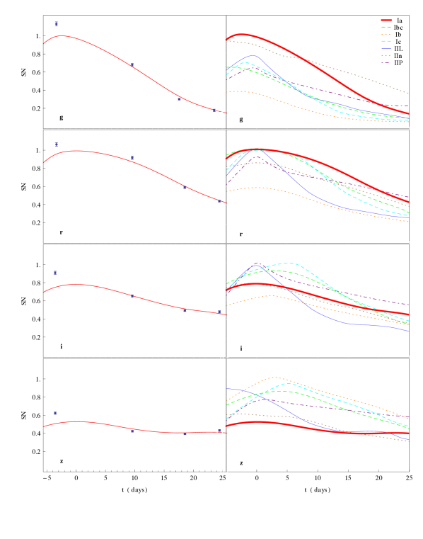
We must now prepare the light curves according the prescription described in section 4. We randomly selected one example of type Ia light curve in SIM1 to illustrate how the fitted functions behave given the data points. This is shown in the left panels of figure 1. The right panels show the light curve functions for different types of non-Ia SNe. Panels from top to bottom run over the DES filters $\{g,r,i,z\}$. In order to facilitate visualization, all curves were normalized as explained in section 4.

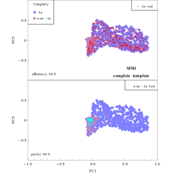
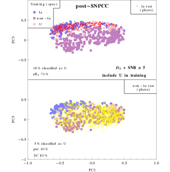
For the SIM1 data set, the cross-validation procedure returns PCs 1 and 5 along with $\sigma=0.3$ as the most appropriate parameters values. The final geometrical distribution of the training sample in such PCs parameter space, along with the classification results are shown in figure 2. In order to facilitate visualization, we show the Ia and non-Ia SNe in the test sample in two different plots.

We can see that, in a best case scenario, KPCA+1NN algorithm is efficient enough to separate the two populations in feature space with a minimum loss in the number of SNe Ia (up to 94% eff_A) and almost no contamination from non-Ia’s in the final sample (up to 99% pur).

5.2.2 Post-SNPCC data

The analysis of the post-SNPCC data was performed in different steps. We first separate a sub-sample which can be consider the analogous of SIM1 inside post-SNPCC, $D_{1}$ with SNR$\geq$5 (hereafter $D_{1}$+SNR5). This data set results from imposing in post-SNPCC data the same selection cuts applied to SIM1.

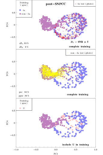
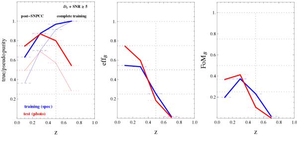
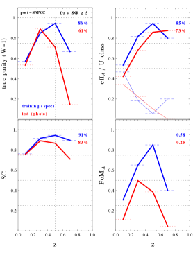
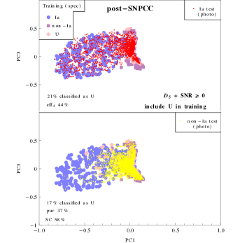
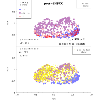
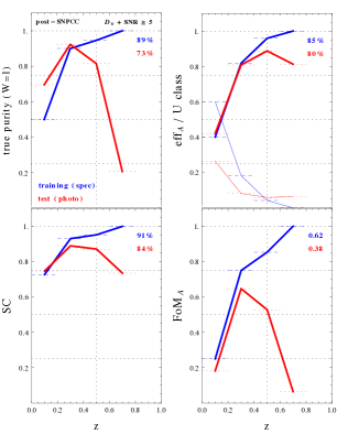
Using $D_{1}$+SNR5, we obtained $89\%$ (80%) pur and SC of $92\%$ (94%) in the training (test) sample. The graphical representation of results from $D_{1}$+SNR5 are shown in the upper and middle panels of Figure 3 and the redshift distribution of the diagnostic parameters are displayed in figures 4 and 22.

Analysing the geometrical distribution of training sample data points (blue circles and purple squares), the numerical results mentioned above become more clear. There is an obvious distinction between the preferential locus occupied by Ia and non-Ia in this parameter space. However, besides the overlapping area where both species exist, and which was already present in SIM1, we can also spot some contamination of non-Ia points inside the area occupied by Ia. Such “misplaced” non-Ia probably gave rise to an important share of the wrong cross-validation classification. In what follows, we described 2 different approaches aimed at suppressing the influence of these “problematic” data points.

The Untyped supernova

Let us focus in $D_{1}$+SNR5 for a moment. Each data point in the training sample is characterized by the SN identification number, its coordinates in PC1 $\times$ PC4 space, the true label and the label from cross-validation. We identified all points who received a wrong label in the cross-validation process and gathered them in a set $U$. We considered these troubled points, in the sense that, although they are spectroscopically confirmed SNe, their light curve characteristics are not enough to fully distinguish them within the training sample.

Figure 7: Classification results obtained for the sub-sample of SNe with FitProb$>$0.1 using different time windows. Red-circles, blue-squares, green-diamonds and gray-triangles correspond to KPCA+1NN results when SNR$\geq 5$, SNR$\geq 3$, SNR$\geq$0 and SNANA cuts are applied, respectively. Horizontal red (dotted), blue (dashed), green (dot-dashed) and gray (full) lines correspond to the results from FitProb criteria for the same set of cuts. Panels show eff_A, pur, FoM_A, SC and the percentage of SNe Ia passing time window requirements from top to bottom.

Our first attempt was to remove all points $\in U$ from the training set before classifying the test sample. In doing so, we defined that a new unlabelled test point would be classified according to the region in the parameter space it occupies, since removing the troubled points defines a clear geometrical boundary between Ia and non-Ia regions in PCs parameter space. This slightly increased our ratings, leading to 87% pur, 93% eff_A, and 96% SC rates.

Trying to get rid of the remaining contamination as much as possible, we consider the complete training sample with 3 different SNe types: Ia, non-Ia and untyped SNe ($U$). This allows us to take advantage of the information in the troubled points and identify light curves similar to them. An expected consequence of this choice is a decrease in efficiency, since some of the Ia in the test sample will be classified as $U$. On the other hand, as the lost of SNe for the $U$ class happens to non-Ia as well, the pur in our final Ia sample will increase, for $D_{1}$+SNR$\geq 5$ to 91%.

The training set divided in 3 sub-samples has its graphical representation shown in the bottom panel of figure 3. For all the cases described here (complete training, excluding $U$ from the training set and including $U$ as a classification type) the distribution of test points will not change, since only the training sample is affected.

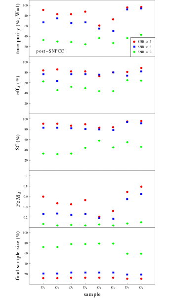
We performed the classification for all samples described in table 1 imposing 3 different SNR cuts (namely SNR$\geq$5, SNR$\geq$3 and SNR$\geq$0). A summary of our finding is detailed in table 5.

Figure 5 shows results for samples listed in the above mentioned table for the case where the $U$ class was included in the training sample as a third SNe type. It is clear from this plot that pur and FoM results become more dependent on time sampling choices as SNR goes higher. The extreme cases being samples $D_{5}$/$D_{6}$ (before maximum, worst results) and $D_{7}$/$D_{8}$ (wider time sampling, better results).

Finally, we should emphasize that our analysis was based on the idea that information should be stored somewhere in the light curve function. If this is true, KPCA could easily be able to provide a direction of information clustering in some untouched feature space, which could be accessed through the data points projections in the PCs. That was the main reason why we started our analysis based on SNR requirements. Errors in flux measurements are direct correlated to the SNR of each observation, and higher errors lead to more oscillations in the light curve functions. In the extreme case were we used random number as components of an input data vector (which contains no information), its projections in PCs will always be located very close to the origin.

Results shown in Table 5 reflects this main idea. Requiring a SNR$\geq$5 in $D_{1}$ to $D_{4}$, we obtained pur, eff_A, and SC rates higher than 80% in all 4 cases. These samples contain approximately 5 times more non-Ia than Ia SNe (see Table 6), which is close to what we expect in a real survey. Beyond that, we did not demand representativeness in redshift or SNe types between the test and training samples. The training sample inside the post-SNPCC data have all the biases the organizers were able to predict and which come along with spectroscopic observational conditions (Kessler et al., 2010). The selection cuts we applied to SNR, in this context, can be seen as a simple procedure to extract the full potential of a given data set.

The results presented here are in agreement to those found by R2012, who applied a diffusion map and random forest algorithm to the same data set. Using the spectroscopic sample as given in the post-SNPCC as a training set, they found 56%/48% for pur/eff_B values. Our analysis for $D_{8}$+SNR0, which imposes no SNR selection cuts, returns 43% pur and 35% eff_B. In their scenario achieving higher purity, they report 90% pur and 8% eff_B from a redshift limited training sample (R2012, Table 6). For $D_{8}$+SNR5, our method achieved 98% pur and 7% eff_B. However, we emphasize that while R2012 uses a different prescription for constructing the training sample, our results were reached using a subset of the spectroscopic sample as it is presented in the SNPCC.

Focusing in sample $S_{m,25}$ of R2012 and cad1+SNR5 of our method, the first feature to call attention is the exponential decay in our results for eff_B. It will be clear in what follows that this is a consequence of SNR cuts (figure 27). In this particular case, we imposed each filter should observe at least 3 epochs with SNR$\geq$5 and, with higher redshift, SNe fulfilling this requirement become rare. Also, in the present analysis, we keep only SNe with observations in all available filters, which prevent us from classifying any object with $z\geq$0.8 (see upper redshift end of our results in figure 4). Obviously these are not intrinsic characteristics of the method, or the data, but choices we made in order to keep results in a conservative perspective. Nevertheless, our values for eff_B are comparable to those of R2012 up to $z\approx 0.4$ (see figure 10 of R2012).

As a consequence, despite the loss in efficiency for the reasons cited above, the local maximum in FoM_B achieved by both groups, us and R2012, are FoM${}_{\rm B}\approx 0.5$, with our method providing higher results up to $z\approx 0.5$.

It was not our purpose to construct a different observation strategy, but instead, to show that if a photometric survey was able to provide a sample similar to post-SNPCC today, it is possible to extract a photometric classified set containing approximately 15% of the entire sample (more than 2000), with SC$\geq$90% . Beyond that, such results can be achieved with minimum astrophysical input and no a priori hypothesis about light curve shape, colour, SNe host environment or redshift.

Results from Linear PCA

Given the wide spread use of linear PCA in astronomy, we also verified how the standard linear version of PCA performs in the SNe photometric classification problem. The method described in section 2.1 was applied to the post-SNPCC data. Once the PCs and projections were calculated, we used a cross-validation algorithm similar to that presented in section 3.2. The main difference being that, in the linear case, there is no parameter $\sigma$ to determine.

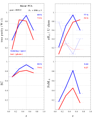
We present results for $D_{1}$ in appendix B. As expected, when no SNR cut is applied, linear and KPCA achieved similar rates of pur and eff_A (table 3). However, when data quality increases, linear PCA is not able to take advantage of the small details introduced in the light-curve function. Results from linear PCA applied to $D_{1}$+SNR5 and including U in training achieved maximum values of 73% pur, 56% eff_A, and 79% SC. Comparing tables 3 and 5, we find that using KPCA for such a case improves results of pur, eff_A, and SC by 25%, 50% and 15% respectively, over the linear PCA outcomes. The dependence of these results with redshift are displayed in figures 4 (for KPCA applied to $D_{1}+$SNR5) and 20 (for the linear case).

Figure 8: Classification results from pre-maximum observations with SNR$\geq$5 ($D_{5}$+SNR5) and considering $U$ as a classification type. The colour code is the same used in figure 3.

Figure 9: Classification results for $t_{\rm low}=-10$, $t_{up}$ being the last point before maximum brightness ($[-10,0[$+SNR5) and considering $U$ as a classification type. The colour code is the same used in figure 3.

Figure 10: Results for pur, eff_A, SC and FoM as a function of redshift for pre-maximum data ($D_{5}+$SNR5) and including U class in the training sample. The top right panel also shows the fraction of SNe classified as U. The colour code is the same used in figure 4.

Figure 11: Redshift dependence results for $[-10,0[$+SNR5 and including U class in the training sample. The panels show the same quantities described in figure 11. The colour code is the same used in figure 4.

5.3 A tougher scenario

In order to make a harder test in the classification power of KPCA+1NN, we used MLCS2k2 light curve fitter within SNANA to exclude easily recognizable non-Ia light curves from the test sample. Once the “obviously” non-Ia are eliminated from the test sample, we were left with a data set containing light curves more similar between each other. If we are able to improve the MLCS2k2 successful classification rates within this sub-sample, we can be sure that the algorithm is doing more than just identifying very strange light curves. We shall see this is the case .

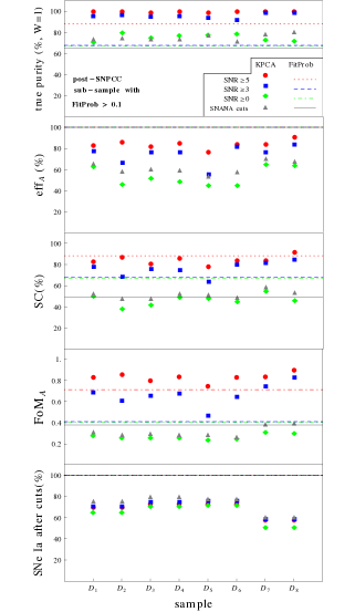
We begin by choosing a selection cut. For each light curve surviving this cut we calculated the fit probability of being a SNe Ia (FitProb) as implemented in SNANA. Those with FitProb$>$0.1 were tagged as Ia and the remaining ones were classified as non-Ia. Figure 6 shows the number of SN according to the calculated FitProb for 4 different selection cuts. Beyond the 3 SNR cuts mentioned previously, we also analysed the outcomes of those used by the SNANA cuts entry submitted to the SNPCC (Kessler et al., 2010). These are defined as: at least 1 observation epoch before maximum brightness, at least 1 epoch after +10 days, at least 1 epoch with SNR$\geq$10 and filters {$r$,$i$} should have maximum SNR$\geq$5. Panels also show results for pur, ppur, eff_A, eff_B, FoM_A and FoM_B obtained from classifying the entire samples according to FitProb. In this plot, it is evident that, no matter which selection cut we choose, there is a high concentration of SNe with FitProb$<$0.1. This reflects the fact that such group of high quality non-Ia light curves are most obviously different from standard SNe Ia, and was responsible for a significant part of our SC rates in the previous sub-section. Analysing the efficiency values, we see that only $\approx 10\%$ of type Ia SNe are wrongly classified as non-Ia according to the FitProb criteria.

We now separate only the SNe classified as Ia according to the FitProb criteria for each selection cut and consider these our entire test sample. After that, we re-calculated the FitProb results and ran the KPCA+1NN classifier. For the SNANA cuts entry, no extra SNR cuts were applied. Results for different time windows are shown in figure 7. From this plot, it is evident that, when no SNR cuts are applied, both methods return very similar results for pur. The FoM_A obtained from the FitProb criteria is higher than those obtained with our method, due the their maximum efficiency in this context (all SNe tagged as Ia). The main difference appears when results for higher SNR are compared. For SNR$\geq 3$, our method is able to increase pur results from pur$\approx 70\%$ to pur$>90\%$ without using any kind of astrophysical information.

In order to have a better idea of how demanding the time sampling is on the SNe Ia sample which already passed the selection cuts, we show in the bottom panel of figure 7 the fraction of SNe Ia that fulfils such requirements. These results are quite similar and almost independent of selection cuts. For $D_{1}$ to $D_{6}$ around $70\%$ of SNe Ia were classifiable and for $D_{7}$ and $D_{8}$ around $60\%$.

5.4 Pre-maximum observations

We also explored the ability of KPCA+1NN to classify light curves given only observation epochs before maximum brightness. A proposal that was submitted to the participants of the SNPCC but did not received any reply. Although such kind of analysis do not produce a SN sample useful for cosmology, it is extremely important in pointing candidates for spectroscopic follow-up.

In a first approach, the light curves were treated as described in section 4. Once the spline fitted functions and time of maximum were obtained, we constructed the data matrix, $\boldsymbol{G}$, with time sampling between -10 e 0 days since maximum brightness ($D_{5}$ and $D_{6}$ in table 1). We emphasize that this scenario uses points after maximum in order to determine $t_{\rm max}$, but not in the construction of matrix $\boldsymbol{G}$. The more realistic situation, where the points after maximum are not used in any step of the process is also analysed bellow.

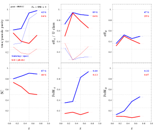
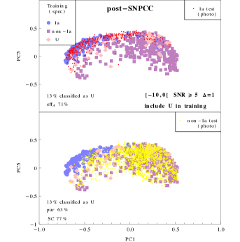
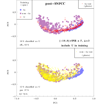
For $D_{5}$+SNR5 and $D_{5}$+SNR0, results are shown in figure 11 and 12, respectively. Figure 11 is similar to figure 3, in the sense that both present a clear separation between Ia and non-Ia points in the training sample and the Ia in the test sample seem to obey that boundary (upper panels). On the other hand, when non-Ia points from the test sample are superimposed, they occupy almost the entire populated region of the parameter space.

In figure 12 the situation changes completely. The effect mention previously, describing data vectors corresponding to low information content localized close to the origin in PC space, is translated into an over-density of points in this area. Beyond that, we also see that the difference between the Ia and non-Ia distributions are not that clear any more. There is a slightly tendency of the non-Ia points agglomerate along the vertical axis, but this entire area is also occupied by Ia. The plot also states that the amount of relevant information contained in Ia input vectors is larger than that in non-Ia, since the spread in the first is much larger than the second. Classification results for $D_{5}$+SNR5 ($D_{5}$+SNR0) achieved 61% (38%) pur, 73% (44%) eff_A and 83% (58%) SC, which leads to a FoM_A of 0.25 (0.07).

We now turn to a more restrict situation. Although very promising, results for $D_{5}$ and $D_{6}$ were not obtained using strictly only pre-maximum data, since the entire light curve was used to determine $t_{\rm max}$ (section 4). In order to analyse a more realistic scenario, we also studied the classification outcomes when points after maximum are removed from the process of determining $t_{\rm max}$.

For each light curve in the post-SNPCC we took just epochs observed before the simulated time of maximum brightness. The spline fit was then applied to these data points and the time of maximum is defined by the r-band as before. If in any other filter the last observed data point correspond to an earlier epoch them $t_{\rm max}$ in $r$-band, we extrapolated the light curve function until it reaches $t_{\rm max}$. We performed classification for $\Delta=1,3$ and in both cases $t_{\rm low}$ was kept as $-10$. After the curves were obtained, we followed the construction of the data matrix $\boldsymbol{G}$ and the KPCA$+$1NN algorithm as explained before. In what follows, these data sample is tagged as $[-10,0[$.

Figure 12: Classification results from pre-maximum observations for $D_{5}$+SNR0. The colour code is the same used in figure 3.

Figure 13: Number of SNe as a function of the difference between the time of maximum brightness determined using the full light-curve (samples $D_{i}$) and using only points before maximum brightness ($[-10,0[$). The upper panel shows histogram for the training sample and the lower panel corresponds to test sample outcomes.

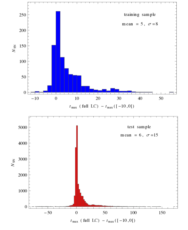
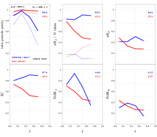
Differences between the time of maximum brightness determined using the entire light curve and using only pre-maximum data are shown in figure 13. Classification results for $[-10,0[$+SNR5 are shown in figure 11 ($\Delta=1$) and 17 ($\Delta=3$) and numerical results for other cases are displayed in table 5. Comparison with results from $D_{5}$+SNR5 (figure 11) shows that, although pur and efficiency remain almost unchanged, there is a larger number of non-Ia classified as $U$. The $U$ type SNe, in this case, acts like a barrier between Ia and non-Ia regions, such that expanding non-Ia cover area (adding data a little more noisy) makes them being classified as $U$ before pur levels are diminished. However, this barrier only works up to a certain point.

Classification results for $D_{6}$ (figure 17) and $[-10,0[$ with $\Delta=3$ (figure 17), both satisfying SNR$\geq$5, reflect this point. The determination of the time of maximum brightness is the only difference between these two data sets, and yet, it is already enough to lower the classification results significantly. A feature that was not verified among the $D_{i}$ samples (figure 5). This demonstrates the importance of a correct determination of the time of maximum brightness. The redshift dependent results for these 2 instances of the data are displayed in figures 17 ($D_{6}$+SNR5) and 17 ($[-10,0[$+SNR5, with $\Delta=3$).

Figure 14: Classification results for $D_{6}$+SNR5. The colour code is the same used in Figure 3.

Figure 15: Classification results for $[-10,0[$+SNR5 with $\Delta=3$. The colour code is the same used in Figure 3.

Figure 16: Results for eff_A, pur, FoM and SC as a function of redshift for $D_{6}+$SNR5. The colour code is the same used in Figure 4.

Figure 17: Results for eff_A, pur, FoM and SC as a function of redshift $[-10,0[+$SNR5 and $\Delta=3$. The colour code is the same used in Figure 4.

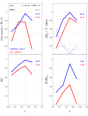
These results are very encouraging. It means that, in the context of future DES data, the algorithm can correctly classify approximately $75\%$ of the initial data sample using only pre-maximum data, if the entire data set was given at once. But in a real situation this can be improved. Suppose that initially, our training sample is composed by the spectroscopic SNe sample available today. As time goes by and pre-maximum light curves are observed, they are automatically classified. An example strategy would be to target with spectroscopic observations the light curves whose projections in PC feature space lay in the boundaries of the SNe Ia/non-Ia regions. Once the SNe type is confirmed, it can be added to the training sample, improving future classification results.

6 SNPCC sample

In order to allow a direct comparison of our results with those reported in the SNPCC, we also applied the KPCA+1NN algorithm to the data set used in the competition. This consists of 20216 simulated light curves of which 1105 represent the spectroscopic sample. This data can be consider less likely to represent the future DES data, given that all bugs listed as fixed “after SNPhotoCC” in table 4 of Kessler et al. (2010) are still part of this sample. However, the application is instructive to have an idea of how our method performs when faced to other algorithms.

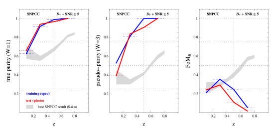
Results for FoM_B, eff_B, ppur (W=3) and pur (W=1) are shown in figure 27 for different SNPCC sub-samples and SNR cuts. This should be compared to figure 5 of Kessler et al. (2010), which reports results from different classifiers without using host galaxy photometric redshift. A detailed analysis of the multiple panels in figure 27 is presented in appendix E.

Our findings from this sample can be summarized through the items bellow:

• There is a weak dependence of the overall classification results with particular time sampling choices. The only eye-catching difference comes from time window including the second maximum in the infrared (D₇).

• Results are highly dependent on SNR cuts, specially efficiency and consequently, FoM.

• D₇+SNR5 achieved FoM_B $>$ 0.25 for 0.2$\leq$ z $\leq$ 0.4. A result only achieved by 3 of the entries participating on the SNPCC (namely Sako, JEDI-KDE and SNANA).

• Our method achieved outstanding pur and ppur results for z$\geq$0.2. In this redshift range, all samples with SNR$\geq$5 reported pur values larger than 75%: a result that was not obtained by none of the SNPCC entries. Particularly, in 0.2$\leq$z$<$0.4, D₇+SNR$\geq$5 obtained 94% $\leq$ pur $\leq$ 97%, while keeping a moderate FoM_B. The redshift dependence of these results are displayed in figure 18.

Figure 18: Classification results for D₇+SNR5 from the SNPCC sample (original SNPCC data set) compared to results reported by the group achieving highest FoM in the SNPCC (Sako). Panels show true purity, pseudo-purity and FoM_B from left to right. Blue (red) lines correspond to results from KPCA+1NN when applied to spectroscopic/training (photometric/test) samples. Gray region correspond to results reported by the group which achieved the best overall classification results in the SNPCC, without using host galaxy photometric redshift information (Kessler et al., 2010).

7 Conclusion

Current SNe surveys already have at hand much more SNe light curves than it is possible to spectroscopically confirm. This situation will increase tremendously in the next decade, which makes SNe Ia photometric identification a crucial issue. In this work, we propose the use of KPCA combined with k = 1 nearest neighbour algorithm (KPCA+1NN) as a framework for SNe photometric classification.

Lately, a large effort has been applied to the SNe photometric classification problem. An up to date compilation of those efforts is reported in Kessler et al. (2010), known as the SuperNova Photometric Classification Challenge (SNPCC). It consisted of a blind simulated light curve sample as expected for the Dark Energy Survey (DES) to be used as a test ground for different classifiers. Although there were some fundamental differences between the algorithms submitted, none of the entries performed obviously better than all the others. After the results were reported, the organizers made public an updated version of the simulated data (post-SNPCC). Both samples, SNPCC and post-SNPCC were analysed in this work.

Our method fit in the class of statistical inference algorithms, according to the SNPCC nomenclature. All calculations are done in the observer frame. There is no corrections due to reddening, local environment, redshift or observation conditions and all available spectroscopically confirmed data surviving quality selection cuts should be used to shape the PCs feature space. The dimensionality reduction is performed using only spectroscopically confirmed SNe (training sample) and each new unlabelled light curve (test sample) is classified one at a time. This allow us to avoid introducing noisy information from non-confirmed SNe in the classifier training. The algorithm is built so that once a new spectroscopic light curve is available or we have total confidence in a photometric one, it can easily be included in the training process, but it is not necessary to redefine the PC feature space every time a new point is to be classified.

In designing our method, we prioritize purity in the final SNe Ia sample, once it is the most important characteristic of a data set to be use for cosmology. We also decided to take a conservative approach towards the unknown features of the data. As a consequence, no extrapolation on time or wavelength domain was used and we demanded that each SNe was observed in all available filters. As expected, these choices have a great impact in our efficiency results. However, we believe that the high purity levels achieved justifies our choices (figure 27), specially in a context where there are already observed light curves not being used for cosmology due to lack of classification (Sako et al., 2011).

We highlight that we chose not to include high complexity in the different steps along the process in order to keep focus in the KPCA performance. Although, as remarked before, there is plenty of room for improvement. For example, in choosing the kernel function, the nearest neighbour algorithm degree and studying more flexible selection cuts. Such developments are worth pursuing, but one should also be aware not to fine tuning the procedure too much, so the results will apply only to one specific data set. Quantifying the dependence of our results with such change of choices is out of the scope of this work.

Results presented in this work show that KPCA+1NN algorithm provide excellent purity in the final SNe Ia sample. Although a time window since maximum brightness needs to be defined, its width does not have a large impact in final classification results. On the other hand, SNR of each observation epoch plays a crucial role. As a consequence, our best results are mainly concentrated in the intermediate range, 0.2$\leq$z$\leq 0.4$. From the SNPCC sample analysis in these redshifts, our method returned FoM_B $>$ 0.25, using D₇+SNR5 (figure 18). A result only achieved by 3 of the entries participating on the SNPCC (namely Sako, JEDI-KDE and SNANA).

We also found outstanding purity and pseudo-purity results. All samples with SNR$\geq$5 reported purity values larger than 75% for z$\geq$0.2: a result that was not obtained by none of the SNPCC entries. Particularly, for 0.2$\leq$ z $\leq$ 0.4, D₇+SNR$\geq$5 obtained 94% $\leq$ pur $\leq$ 97%, while keeping a moderate FoM (figure 18).

Among the entries submitted to the SNPCC, only the InCA group used a similar approach, although by means of completely different techniques. The results they reported to the competition provide purity rates similar the ones we get for SNR$\geq 0$.

We stress that, although the comparison with the SNPCC results is important, it cannot be considered exactly in the same grounds as our results. First because since they were built with different purposes (the SNPCC aimed at maximum FoM_B and our goal was to achieve the highest possible purity while maintaining a reasonable FoM), second because we were not time constrained as the groups taking the challenge and finally, we had access to the answer key before hand. Something the competitors did not have. However, a strictly direct comparison with other results in the literature is possible through the post-SNPCC sample.

Recently, the InCA group made public a detailed analysis of the results achieved by their method when applied to the post-SNPCC data set (Richards et al., 2012) (R2012). The two algorithms provided similar classification results. Both achieving local maximum of FoM_B around 0.5, with our method giving better results at lower and theirs at higher redshifts. Averaging over the entire redshift range, we achieve FoM_B of 0.06 and R2012 reported 0.35. R2012 also provides results with different spectroscopic samples, constructed by re-distributing DES available follow-up time. In their result with highest purity, they reported 90% purity, 8% eff_B and 0.08 FoM_B using a redshift limited spectroscopic sample. Our method provides 96% purity, 6% eff_B and 0.06 FoM_B for $D_{7}$+SNR$\geq$5.

Karpenka et al. (2012) also present results from post-SNPCC data. In their analysis, results from a parametric fit to the spectroscopic light curves are used to train a neural network which subsequently returns the probability of a new object being a Ia. Using 50% of the initial sample as a training set ($\approx$10000 objects considered spectroscopically confirmed), they found 80% purity, 85% eff_B and 0.51 FoM_B.

It is important to emphasize that the results we report above were achieved using a sub-set of the spectroscopic sample as it is given within the post-SNPCC data. This means that it is not necessary to tailor the spectroscopic sample a priori in order to get high purity results, making our method ideal as a first approach to a large photometric data set.

In order to test the algorithm in a more restrictive scenario, we present results obtained from the post-SNPCC sub-sample with MultiColor Light-curve Shape (MLCS2k2) fit probability, FitProb$>0.1$. This sample contains light curves very similar between each other, and represents a more difficult classification challenge than the complete SNPCC data. We show that our method is not able to do more than identifying the obviously non-Ia light curves when no SNR cuts are applied. However, when we compare results from data samples with SNR$\geq$3, KPCA+1NN can boost purity levels to $>95\%$ independently of time window sampling.

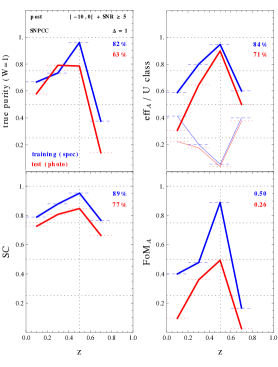
Finally, we report the first attempt in classifying the post-SNPCC data using only pre-maximum epochs. This study is very important in selecting candidates for spectroscopic follow up. Using only data between -10 and 0 days since maximum brightness, we obtained 63% purity, 71% eff_A, 77% SC and FoM_A of 0.26. This is a very enthusiastic result and reflects the vast room for improvement this kind of analysis may provide in different stages of the pipeline.

We stress that the application proposed here is merely an example of how the KPCA$+$kNN algorithm might be applied in astronomy. Beyond the specific problem of SNe Ia photometric classification, the same procedure can be used to identify other expected transient sources and even to spot still non-observed objects among a large and heterogeneous data set. The projection of such objects in PCs feature space would occupy a previously non-populated locus, what would give us a hint to further investigate that particular object. In the more ideal scenario, when synthetic light curves from a non-observer object is available, a synthetic target can be included in the training sample, leading to a detection tailored according to our expectations. This provides still another advantage over template fitting techniques, which deserve further investigation.

From what was presented here, we conclude that the decision of choosing one method over the other is not a straightforward one, but must be balanced by the characteristics of the data available and our goal in classifying it. Given that SNe without spectroscopic confirmation is not a future issue of large surveys, but a problem that is already present in the SDSS data (Sako et al., 2011), KPCA+1NN algorithm proved to be the ideal choice to quickly increase the number of SNe Ia available for cosmology with minimum contamination. Alternatively, it can also be used as a complement to other techniques in helping to increase the number of SNe Ia in the training sample. Either way, we have enough evidence to trust the competitiveness of our algorithm within the current status of the SNe photometric classification field.

Appendix A Basic proofs

This appendix contain basic proofs for the statements used throughout the text. These are common to machine learning theory field, but may not be as such for the astronomy community. They follow closely Max Welling’s notes A first encounter with Machine Learning and Schölkopf et al. (1996), which the reader is advised to check for a comprehensible introduction to the basic concepts used here.

1. All the vectors in the eigenvector space $V$ lie in the space spanned by the data vectors contained in $X$

   Consider $\mathbf{v}_{a}\in V$,

   $$\lambda_{a}\mathbf{v}_{a} = C\mathbf{v}_{a}=\frac{1}{N}\sum_{i=1}^{N}\mathbf{x}_{i}\mathbf{x}_{i}^{T}\mathbf{v}_{a}=\frac{1}{N}\sum_{i=1}^{N}\left(\mathbf{x}_{i}^{T}\mathbf{v}_{a}\right)\mathbf{x}_{i}$$

   $$\Rightarrow$$

   $$\mathbf{v}_{a} = \sum_{i=1}^{N}\left[\frac{\left(\mathbf{x}_{i}^{T}\mathbf{v}_{a}\right)}{N\lambda_{a}}\right]\mathbf{x}_{i}=\sum_{i=1}^{N}\alpha_{i}\mathbf{x}_{i}.$$ (21)

   In other words, any eigenvector can be written as a linear combination of the vectors in $X$ and, as a consequence, must lie in the space spanned by them.
   

2. Determining equation (7)

   Consider the projected eigenvalue equations,

   $$\mathbf{x}_{i}^{T}C\mathbf{v}_{a}=\lambda_{a}\mathbf{x}_{i}^{T}\mathbf{v}_{a}.$$ (22)

   Using equations (2) and (5), we have

   $$\mathbf{x}_{i}^{T}\frac{1}{N}\sum_{j=1}^{N}\mathbf{x}_{j}\mathbf{x}_{j}^{T}\sum_{k=1}^{N}\alpha_{k}^{a}\mathbf{x}_{k} = \lambda_{a}\mathbf{x}_{i}^{T}\sum_{l=1}^{N}\alpha_{l}^{a}\mathbf{x}_{l}$$ (23)

   $$\frac{1}{N}\sum_{j,k}\alpha_{k}^{a}\left[\mathbf{x}_{i}^{T}\mathbf{x}_{j}\right]\left[\mathbf{x}_{j}^{T}\mathbf{x}_{k}\right] = \lambda_{a}\sum_{l=1}^{N}\alpha_{l}^{a}\left[\mathbf{x}_{i}^{T}\mathbf{x}_{l}\right].$$

   Addressing $K_{ij}=\left[\mathbf{x}_{i}^{T}\mathbf{x}_{j}\right]$, we can write

   $$K\boldsymbol{\alpha}^{a}=\tilde{\lambda_{a}}\boldsymbol{\alpha}^{a}\qquad{\rm where}\qquad\tilde{\lambda}=N\lambda_{a}.$$ (24)

   
   

3. Determination of $||\boldsymbol{\alpha}^{a}||$
   The norm of parameters $\boldsymbol{\alpha}^{a}$ is a consequence of the normalization of the eigenvectors in $V$.Using equation (5),

   $$\mathbf{v}_{a}^{T}\mathbf{v}_{a}=1\qquad \Rightarrow \qquad\sum_{i,j}\alpha_{i}^{a}\alpha_{j}^{a}\left[\mathbf{x}_{i}^{T}\mathbf{x}_{j}\right]=\left(\mathbf{\alpha}^{a}\right)^{T}K\mathbf{\alpha^{a}}=1$$ (25)

   $$\Rightarrow \qquad N\lambda_{a}\left(\boldsymbol{\alpha}^{a}\right)^{T}\boldsymbol{\alpha}^{a}=1$$

   $$\Rightarrow \qquad||\boldsymbol{\alpha}^{a}||=\frac{1}{\sqrt{N\lambda_{a}}}.$$

   
   

4. Obtaining $K_{F}$ and $\boldsymbol{\alpha}_{\Phi}$

   We begin with the definition of the covariance matrix in feature space

   $$C_{\rm F}=\frac{1}{N}\sum_{i=1}^{N}\Phi(x_{i})\Phi(x_{i})^{T},$$ (26)

   we have to find the eigenvalues, $\lambda_{\Phi}$, and eigenvectors, $\mathbf{v}_{\Phi}$, which satisfy

   $$\lambda_{\Phi}\mathbf{v}_{\Phi}=C_{\rm F}\mathbf{v}_{\Phi}.$$ (27)

   Using item (ii) above, we have that all $\mathbf{v}_{\Phi}$ can be written as a linear combination of the $\Phi$’s. This means that we are allowed to consider the equivalent equations

   $$\lambda_{\Phi}\left(\Phi(\mathbf{x}_{k})\cdot\mathbf{v}_{\Phi}\right)=\left(\Phi(\mathbf{x}_{k})\cdot C_{F}\mathbf{v}_{\Phi}\right),\qquad\forall k,$$ (28)

   with the prescription that

   $$\mathbf{v}_{\Phi}=\sum_{i=1}^{N}\alpha_{\Phi}^{i}\Phi(\mathbf{x}_{i}).$$ (29)

   Using equations (28) and (29),

   $$\lambda_{\Phi}\sum_{i=1}^{N}\alpha_{\Phi}^{i}\left(\Phi(\mathbf{x}_{k})\cdot\Phi(\mathbf{x}_{i})\right)=$$ (30)

   $$= \frac{1}{N}\sum_{i=1}^{N}\alpha_{\Phi}^{i}\left(\Phi(\mathbf{x}_{k})\cdot\sum_{j=1}^{N}\Phi(\mathbf{x}_{j})\right)\left(\Phi(\mathbf{x}_{j})\cdot\Phi(\mathbf{x}_{i})\right).$$

   Calling

   $$\left(K_{F}\right)_{ij}:=\left(\Phi(\mathbf{x}_{i})\cdot\Phi(\mathbf{x}_{j})\right),$$ (31)

   leads to

   $$N\lambda_{\Phi}K_{F}\boldsymbol{\alpha}=K_{F}^{2}\boldsymbol{\alpha},$$ (32)

   where $\boldsymbol{\alpha}$ is a column vector. As $K_{F}$ is symmetric,

   $$K_{F}\boldsymbol{\alpha}=\widetilde{\lambda_{\Phi}}\boldsymbol{\alpha},$$ (33)

   with $\widetilde{\lambda_{\Phi}}=N\lambda_{\Phi}$. In order to obtain $\boldsymbol{\alpha}_{\Phi}$, we only need to diagonalize $KF$.

   The normalization of $\boldsymbol{\alpha}_{\Phi}$ is achieved by requiring

   $$\left(\mathbf{v}_{\Phi}^{k}\cdot\mathbf{v}_{\Phi}^{k}\right)=1,\qquad\forall k.$$ (34)

   Through equations (29) and (33) this converts into

   $$1 = \sum_{i,j=1}^{N}\left[\alpha_{\Phi}^{k}\right]_{i}\left[\alpha_{\Phi}^{k}\right]_{j}\left(\Phi(\mathbf{x}_{i})\cdot\Phi(\mathbf{x}_{j})\right)$$ (35)

   $$= \sum_{i,j=1}^{N}\left[\alpha_{\Phi}^{k}\right]_{i}\left[\alpha_{\Phi}^{k}\right]_{j}{K_{F}}_{ij}$$

   $$= \left(\boldsymbol{\alpha}^{k}\cdot K_{F}\boldsymbol{\alpha}_{\Phi}^{k}\right)$$

   $$= \lambda_{\Phi}^{k}\left(\boldsymbol{\alpha}_{\Phi}^{k}\cdot\boldsymbol{\alpha}_{\Phi}^{k}\right).$$

   
   

5. Centralization in feature space

   Considered the centred vectors in feature space

   $$\widetilde{\Phi}(\mathbf{x}_{i}):=\Phi(\mathbf{x}_{i})-\frac{1}{N}\sum_{i=1}^{N}\Phi(\mathbf{x}_{i}),$$ (36)

   our goal now is to define the dot product matrix

   $$\widetilde{K_{F}}_{ij}=\widetilde{\Phi}(\mathbf{x}_{i})^{T}\widetilde{\Phi}(\mathbf{x}_{j}).$$ (37)

   In a procedure similar to (v) above, we arrive at the eigenvalue equation

   $$\widetilde{\lambda}_{\Phi}\widetilde{\boldsymbol{\alpha}}_{\Phi}=\widetilde{K_{F}}\widetilde{\boldsymbol{\alpha}}_{\Phi},$$ (38)

   which has eigenvectors $\widetilde{\mathbf{v}_{\Phi}}$ and

   $$\widetilde{\mathbf{v}_{\Phi}}=\sum_{i=1}^{N}\widetilde{\boldsymbol{\alpha}}_{i}\widetilde{\Phi}(\mathbf{x}_{i}).$$ (39)

   In this case, we do not have the centered data points represented by equation (36), so we need to write $\widetilde{K_{F}}$ in terms of $K_{F}$. In what follows, consider $1_{ij}=1,\forall i,j$.

   Using equations (36) and (37),

   $$\widetilde{K_{F}}_{ij} = \widetilde{\Phi}(\mathbf{x}_{i})^{T}\widetilde{\Phi}(\mathbf{x}_{j})$$

   $$= \left(\Phi(\mathbf{x}_{i})-\frac{1}{N}\sum_{m=1}^{N}\Phi(\mathbf{x}_{m})\right)^{T}\times$$

   $$\times\left(\Phi(\mathbf{x}_{j})-\frac{1}{N}\sum_{n=1}^{N}\Phi(\mathbf{x}_{n})\right)$$

   $$= \Phi(\mathbf{x}_{i})^{T}\Phi(\mathbf{x_{j}})-\frac{1}{N}\sum_{m=1}^{N}\Phi(\mathbf{x}_{m})^{T}\Phi(\mathbf{x}_{j})$$

   $$-\frac{1}{N}\sum_{n=1}^{N}\Phi(\mathbf{x}_{i})^{T}\Phi(\mathbf{x}_{n})$$

   $$+\frac{1}{N^{2}}\sum_{n,m=1}^{N}\Phi(\mathbf{x}_{m})^{T}\Phi(\mathbf{x}_{n})$$

   $$= {K_{F}}_{ij}-\frac{1}{N}\sum_{i=1}^{M}1_{im}{K_{F}}_{mj}$$

   $$-\frac{1}{N}\sum_{n=1}^{N}{K_{F}}_{in}1_{nj}+\frac{1}{N^{2}}\sum_{n,m=1}^{N}1_{im}{K_{F}}_{mn}1_{nj}.$$

   Considering $\left(1_{N}\right)_{ij}:=1/N,\quad\forall\quad\{i,j\}$, we have the shorter version,

   $$\widetilde{K_{F}}=K_{F}-1_{N}K_{F}-K_{F}1_{N}+1_{N}K_{F}1_{N}.$$ (41)

Appendix B Linear PCA

Figure 19: Classification results using linear PCA for $D_{1}$+SNR5. The colour code is the same used in Figure 3.

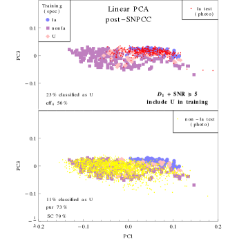
We present here the results we achieved from applying linear PCA to the post-SNPCC data. The procedure for deriving the PCs are described in subsection 2.1. The 2 PCs that best separate Ia and non-Ia data points were identified by using a cross-validation algorithm similar to the one described in subsection 3.2. The only difference is that, in the linear case, there is no parameter $\sigma$ to adjust. The outcomes for sample $D_{1}$ using different SNR cuts are displayed in table 3. The graphical representation of data points projections for the SNR$\geq$5 case is shown in figure 19 and the redshift dependence of the classification results are displayed in figure 20.

Comparing results for $D_{1}$+SNR5 when U class is included in the training, presented in Tables 3 and 5, the reader can verify that the using KPCA raises the efficiency levels from 56% to 84% and the purity levels from 73% to 91%. This corresponds to approximately 50% increase in efficiency and 25% increase in purity.

Table 3: Results from applying linear PCA+1NN to the post-SNPCC data, $D_{1}$ sample. Ratios of efficiency (eff), purity (pur) and successful classification (SC) are reported in percentages (%).

		Training sample			Test sample
		cross-validated			including U
	PC pair	effA	pur	SC	effA	pur	SC	FoMA
SNR$\geq$5	1-3	77	80	86	56	73	79	0.27
SNR$\geq$3	1-3	85	83	87	64	63	78	0.23
SNR$\geq$0	1-3	84	84	84	48	32	50	0.07

Figure 20: Classification results for $D_{1}+$SNR5 as a function of redshift using linear PCA. The color code is the same used in figure 4.

Appendix C Results for $D_{1}$ as a function of redshift and SNR cuts

Figure 21: Test sample classification results of efficiency, purity, FoM and SC for $D_{1}$ as a function of redshift. The orange (dot-dashed), brown (dashed) and green (dotted) lines correspond to SNR$\geq$5, SNR$\geq$3 and SNR$\geq$0, respectively.

Figure 22: Results from the post-SNPCC data for SC (left), eff_A (middle) and FoM_A as a function of redshift for $D_{1}+$SNR5. The color code is the same used in figure 4. Top-middle panel also shows values of the percentage of SNe classified as $U$ (thin lines, blue for training and red for test sample).

Figure 23: Results from the post-SNPCC data for pur (top-right), eff_A (top-middle), eff_B (top-right), SC (bottom-left), FoM_A (bottom-middle) and FoM_B (bottom-right) as a function of redshift for $D_{1}+$SNR5 and including U class in the training sample. The color code is the same used in figure 4. Top-left and top-middle panels also show values of pseudo-purity and the percentage of SNe classified as $U$ (thin lines, blue for training and red for test sample), respectively.

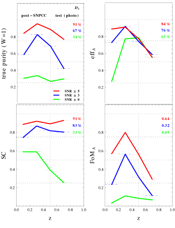
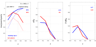
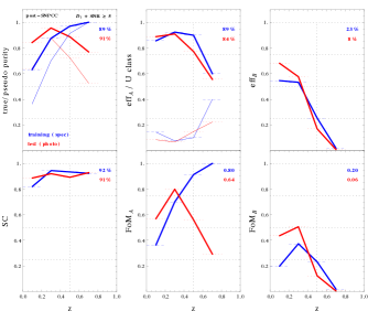
Figure 21 shows how the classification results for $D_{1}$ (test sample) behave as a function of redshift and SNR selection cuts. Figure 22 shows SC, efficiency and FoM results normalized after election cuts.

Examining the top-middle panel of figure 23, we see that eff_A also suffers in high redshift due to SNe classified as $U$ (thin lines). This was another choice we made in order to preserve purity. Although a few SNe Ia are lost to the $U$ class (which is bad for efficiency), so are non-Ia that would easily be mistaken with SNe Ia (which is good for purity). This effect becomes clear if we compare figures 4 and 22 to figure 23. From these we see that eff_A gets from 89% (without $U$ type) to 84% (with $U$ type) but at the same time purity increased from 80% to 91%, staying above 75% for the entire redshift range.

Appendix D $D_{8}$+SNR0 classifications

Figure 24: Classification results for $D_{8}$+SNR0, including U class in the training sample. The color code is the same used in figure 3.

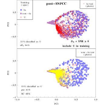
We present in figures 24, 26 and 26 the classification results for $D_{8}$+SNR0. This is shown in order to facilitate comparison with other methods from the literature which do not apply SNR cuts. However, we emphasize that, for a given time sampling, this is the worst case scenario for our method. As shown in figure 21, the classification potential of the method is highly increased with better quality data (higher SNR).

Figure 25: Classification results as a function of redshift for Ia ($D_{8}$+SNR0), including U class in the training sample. The panels show efficiency, purity, FoM and SC from top to bottom. The colour code is the same used in figure 4.

Figure 26: Analogous of figure 26 for non-Ia classifications.

Appendix E SNPCC complete results

Figure 27 shows detailed results obtained from the SNPCC sample for different time window samplings. It is composed by 4 big panels, each one containing plots for a diagnostic parameter, organized in 3 rows and 4 columns. The rows run through SNR$\geq$5, SNR$\geq$3 and SNR$\geq 0$, from top to bottom. The left-most column in each panel show results for SNR cuts only. Meaning that all SNe surviving the corresponding SNR cut were classified as Ia. Other columns represent $D_{1}$, $D_{3}$ and $D_{7}$, from left to right. Outcomes from $D_{2}$, $D_{4}$ and $D_{8}$ are similar to the ones presented in the plot, so we decided not to show them.

The first thing to notice from this figure is that the time window sampling leads to small differences in the overall classification results. Obviously higher purity results comes from $D_{7}$, the only sub-sample which includes the second maximum in the infra-red, for SNe Ia in $z\leq 0.8$. However, discrepancies between results from different SNR cuts are much larger. This shows that, despite the need to define a time window, the specific choice is not crucial in the determination of final results.

The same argument does not hold for SNR selection cuts. We see the crucial role played by the quality of each observation, no matter which diagnostic we analyse. Although this effect is noticeable in all of them, it is more evident in outcomes from eff_B and FoM_B, due to reasons already discussed in section 5. Nevertheless, our method achieved FoM${}_{\rm B}>0.25$ for $z\leq 0.25$. In this redshift range, only SNPCC entries Sako, JEDI-KDE and SNANA cuts reported comparable results. The behaviour of our eff_B plots is almost opposite to what is reported from the SNPCC. In those, the efficiency is almost always very high, what frequently comes accompanied by a low purity result.

On the other hand, our results for purity and pseudo-purity are very good, specially for redshifts within $[0.2,0.5]$. For all sub-samples with SNR$\geq$5, we achieved purity values larger than 75% in this redshift range, a result that is not present in none of the entries in the SNPCC. Beyond that, $D_{7}$+SNR$\geq$5 gives good results for purity and pseudo-purity for $z\geq 0.5$, confirming the importance of observing the second maximum in the infra-red.

Figure 27: Redshift dependence results from the SNPCC data set for FoM_B (top-left), eff_B (top-right), pseudo-purity (bottom-left) and true purity (bottom-right), including $U$ as an extra class in the training sample. The blue-thick lines correspond to results from the training (spectroscopic) sample and the red-thick to results from the test (photometric) sample. The left-most columns in each big panel show results where all SNe satisfying the SNR selection cuts were tagged as Ia. Rows run through SNR cuts: SNR$\geq$5, SNR$\geq$3 and SNR$\geq$0 from top to bottom. Columns 2 to 4 show results for $D_{1}$, $D_{3}$ and $D_{5}$, from left to right.

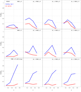
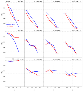
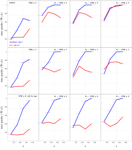
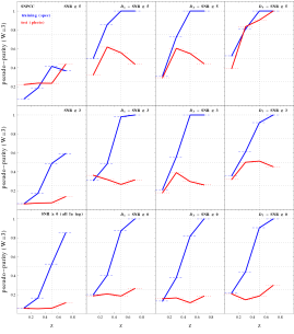
Appendix F Summary tables

We present bellow complete tables describing our results for different light curve time samplings and SNR cuts.

Table 4: Number of SNe in each post-SNPCC subset. The table also shows subsamples of the $D_{i}$ and $[-10,0[$ according to SNR cuts.

		Training sample
			$D_{1}$			$D_{3}$			$D_{5}$			$D_{7}$
	SIM1		SNR$\geq$0	SNR$\geq$3	SNR$\geq$5	SNR$\geq$0	SNR$\geq$3	SNR$\geq$5	SNR$\geq$0	SNR$\geq$3	SNR$\geq$5	SNR$\geq$0	SNR$\geq$3	SNR$\geq$5
Ia	559		374	213	142	409	225	145	418	232	148	297	173	119
non-Ia	544		355	315	273	397	347	303	412	350	303	282	257	222
total	1103		729	528	415	806	572	448	830	582	415	579	430	341
			Test sample
			$D_{1}$			$D_{3}$			$D_{5}$			$D_{7}$
	SIM1		SNR$\geq$0	SNR$\geq$3	SNR$\geq$5	SNR$\geq$0	SNR$\geq$3	SNR$\geq$5	SNR$\geq$0	SNR$\geq$3	SNR$\geq$5	SNR$\geq$0	SNR$\geq$3	SNR$\geq$5
Ia	559		3181	633	431	3480	666	453	3575	673	448	2525	520	354
non-Ia	544		11346	3716	1993	12255	3926	2100	12413	3900	2096	9340	3241	1776
total	1103		14527	4349	2424	15735	4592	2553	15988	4573	2544	11865	3761	2130
				Test sample				Training Sample
				$[-10,0[$				$[-10,0[$
				SNR$\geq$0	SNR$\geq$3	SNR$\geq$5		SNR$\geq$0	SNR$\geq$3	SNR$\geq$5
			Ia	444	238	153		3555	661	437
			nonIa	440	361	312		12544	3926	2125
			total	884	599	465		16099	4587	2562

Table 5: Summary of classifications results for post-SNPCC data. Ratios of efficiency (eff_A/eff_B), purity (pur) and successful classification (SC) are reported in percentages (%).

							Test sample
				Training sample			complete			exclude U			include U
				cross validated
data set	SNR	$\sigma$	PCs	effA	pur	SC	effA	pur	SC	effA	pur	SC	effA	pur	SC	FoMA	effB	FoMB
$D_{1}$	$\geq 5$	0.9	$1\quad 4$	89	89	92	89	80	94	93	87	96	84	91	91	0.64	8	0.06
	$\geq 3$	0.9	$1\quad 2$	87	86	89	83	56	88	89	64	91	76	67	83	0.32	11	0.04
	$\geq 0$	0.7	$1\quad 5$	88	87	87	73	30	57	81	24	41	63	34	33	0.09	44	0.06
$D_{2}$	$\geq 5$	0.4	$1\quad 3$	90	90	92	90	77	94	93	80	95	86	83	91	0.54	8	0.05
	$\geq 3$	0.7	$1\quad 5$	88	88	90	77	62	90	78	70	92	64	75	83	0.32	9	0.04
	$\geq 0$	0.4	$1\quad 5$	86	88	87	65	32	63	87	27	46	32	30	32	0.06	46	0.04
$D_{3}$	$\geq 5$	1.0	$1\quad 2$	84	86	90	89	71	92	91	75	93	82	83	87	0.51	8	0.05
	$\geq 3$	1.0	$1\quad 2$	85	87	89	84	52	86	88	58	89	77	67	82	0.31	11	0.05
	$\geq 0$	0.6	$1\quad 4$	85	84	84	69	30	58	79	26	45	52	29	34	0.06	40	0.05
$D_{4}$	$\geq 5$	0.3	$1\quad 4$	85	90	92	87	78	93	88	86	95	82	88	91	0.58	8	0.06
	$\geq 3$	0.6	$1\quad 2$	83	86	88	85	53	87	88	57	89	77	67	81	0.31	11	0.05
	$\geq 0$	1.7	$1\quad 3$	85	85	85	60	26	53	62	25	51	50	25	44	0.05	38	0.04
$D_{5}$	$\geq 5$	1.9	$1\quad 3$	85	86	91	82	59	87	88	60	87	73	61	83	0.25	-	-
	$\geq 3$	1.1	$1\quad 3$	87	91	91	85	48	84	87	53	87	76	56	80	0.22	-	-
	$\geq 0$	0.4	$1\quad 3$	82	85	84	56	34	65	57	38	69	44	38	58	0.07	-	-
$D_{6}$	$\geq 5$	0.8	$1\quad 3$	85	89	91	86	62	88	87	69	91	80	73	84	0.38	-	-
	$\geq 3$	1.0	$1\quad 3$	88	90	91	86	45	83	91	48	84	81	51	79	0.21	-	-
	$\geq 0$	1.3	$1\quad 3$	86	85	85	60	28	57	52	25	55	44	27	45	0.05	-	-
$D_{7}$	$\geq 5$	0.5	$1\quad 2$	93	92	95	86	95	97	86	96	97	81	96	95	0.72	6	0.06
	$\geq 3$	0.6	$1\quad 2$	91	90	92	80	86	96	84	90	97	74	92	95	0.59	9	0.07
	$\geq 0$	1.3	$1\quad 2$	90	87	88	72	36	66	77	35	64	65	37	55	0.11	36	0.06
$D_{8}$	$\geq 5$	0.4	$1\quad 2$	92	90	94	90	92	97	92	96	98	89	98	96	0.83	7	0.06
	$\geq 3$	0.5	$1\quad 2$	91	89	92	84	76	94	88	92	97	82	94	92	0.69	9	0.08
	$\geq 0$	0.7	$1\quad 2$	89	86	87	74	41	71	94	33	58	64	43	46	0.13	35	0.07
$[-10,0[$	$\geq 5$	1.2	$1\quad 5$	84	82	89	78	53	85	78	60	87	71	63	77	0.26	-	-
	$\geq 3$	1.4	$1\quad 5$	81	81	85	76	35	76	77	40	80	67	43	67	0.13	-	-
$\Delta=1$	$\geq 0$	1.6	$1\quad 5$	80	81	81	65	28	56	67	29	56	52	30	45	0.06	-	-
$[-10,0[$	$\geq 5$	0.9	$1\quad 5$	86	81	89	69	51	83	74	51	84	63	57	76	0.20	-	-
	$\geq 3$	1.6	$1\quad 3$	84	87	89	85	41	80	86	46	84	78	50	76	0.19	-	-
$\Delta=3$	$\geq 0$	1.2	$1\quad 3$	81	82	81	74	37	67	75	40	70	58	44	54	0.12	-	-

Table 6: Number of SNe in each SNPCC subset. The table also shows sub-samples of the $D_{i}$ according to SNR cuts.

	Training sample
	$D_{1}$			$D_{3}$			$D_{7}$
	SNR$\geq$0	SNR$\geq$3	SNR$\geq$5	SNR$\geq$0	SNR$\geq$3	SNR$\geq$5	SNR$\geq$0	SNR$\geq$3	SNR$\geq$5
Ia	546	311	216	601	330	601	455	272	188
non-Ia	278	254	225	312	283	312	242	221	199
total	824	565	441	913	613	913	697	493	388
	Test sample
	$D_{1}$			$D_{3}$			$D_{7}$
	SNR$\geq$0	SNR$\geq$3	SNR$\geq$5	SNR$\geq$0	SNR$\geq$3	SNR$\geq$5	SNR$\geq$0	SNR$\geq$3	SNR$\geq$5
Ia	2713	2201	972	2942	2366	1019	2303	1904	956
non-Ia	9785	6651	2262	10372	6969	2338	8411	6139	2185
total	12498	8852	3234	13314	9335	3357	10714	8043	3141

Table 7: Summary of classifications results for SNPCC sub-samples. Results for efficiency before (eff_B) and after (eff_A) selection cuts, purity (pur) and successful classification (SC) are reported in percentages (%).

							Test sample
				Training sample			include U
				cross validated
data set	SNR	$\sigma$	PCs	effA	pur	SC	effA	pur	SC	FoMA	effB	FoMB
$D_{1}$	$\geq 5$	1.0	$1\quad 5$	94	96	95	32	75	75	0.16	7	0.03
	$\geq 3$	0.9	$1\quad 5$	91	89	89	50	55	66	0.15	24	0.07
	$\geq 0$	0.8	$1\quad 4$	87	88	84	58	50	63	0.15	35	0.09
$D_{2}$	$\geq 5$	0.6	$1\quad 5$	94	96	95	32	77	75	0.17	7	0.04
	$\geq 3$	0.6	$1\quad 5$	91	91	90	47	53	69	0.13	23	0.06
	$\geq 0$	1.0	$1\quad 2$	88	89	85	59	34	49	0.09	36	0.05
$D_{3}$	$\geq 5$	0.7	$1\quad 5$	90	92	92	30	73	71	0.14	7	0.03
	$\geq 3$	0.6	$1\quad 2$	87	89	87	35	56	41	0.10	18	0.05
	$\geq 0$	0.8	$1\quad 3$	86	86	81	64	36	39	0.10	41	0.07
$D_{4}$	$\geq 5$	0.5	$1\quad 5$	91	92	92	30	72	72	0.14	7	0.03
	$\geq 3$	0.4	$1\quad 4$	87	88	87	42	33	56	0.06	22	0.05
	$\geq 0$	1.7	$1\quad 3$	87	89	86	32	32	48	0.09	40	0.06
$D_{7}$	$\geq 5$	0.8	$1\quad 4$	92	93	93	27	91	72	0.21	6	0.04
	$\geq 3$	0.8	$1\quad 2$	91	91	90	34	68	74	0.14	15	0.06
	$\geq 0$	1.0	$1\quad 5$	93	90	89	55	48	64	0.13	28	0.07
$D_{8}$	$\geq 5$	1.2	$1\quad 4$	93	93	93	54	74	64	0.26	11	0.06
	$\geq 3$	1.1	$1\quad 4$	91	93	91	59	51	66	0.15	26	0.07
	$\geq 0$	0.8	$1\quad 5$	89	88	86	63	43	42	0.12	32	0.06

References

- Arlot & Celisse (2010) Arlot S., Celisse A., 2010, Statistics Surveys, 4, 40
- Astier et al. (2006) Astier P., Guy J., Regnault N., Pain R., Aubourg E., Balam D., Basa S., Carlberg R. G., et al. 2006, A&A, 447, 31
- Ball & Brunner (2010) Ball N. M., Brunner R. J., 2010, International Journal of Modern Physics D, 19, 1049
- Benitez-Herrera et al. (2012) Benitez-Herrera S., Röpke F., Hillebrandt W., Mignone C., Bartelmann M., Weller J., 2012, MNRAS, 419, 513
- Beyer et al. (1999) Beyer K., Goldstein J., Ramakrishnan R., Shaft U., 1999, in Int. Conf. on Database Theory When is ”nearest neighbor” meaningful?. pp 217–235
- Blake et al. (2011) Blake C., Kazin E. A., Beutler F., Davis T. M., Parkinson D., Brough S., Colless M., Contreras C., et al. 2011, MNRAS, 418, 1707
- Conley et al. (2011) Conley A., Guy J., Sullivan M., Regnault N., Astier P., Balland C., Basa S., Carlberg R. G., et al. 2011, ApJS, 192, 1
- Falck et al. (2010) Falck B. L., Riess A. G., Hlozek R., 2010, ApJ, 723, 398
- Gong et al. (2010) Gong Y., Cooray A., Chen X., 2010, ApJ, 709, 1420
- Hofmann et al. (2008) Hofmann B., Schölkopf B., Smola A., 2008, The Annals of Statistics, 36, 1171
- Ishida & de Souza (2011) Ishida E. E. O., de Souza R. S., 2011, A&A, 527, A49
- Ishida et al. (2011) Ishida E. E. O., de Souza R. S., Ferrara A., 2011, MNRAS, 418, 500
- James (1998) James G., 1998, PhD thesis, Stanford University
- Jha et al. (2007) Jha S., Riess A. G., Kirshner R. P., 2007, ApJ, 659, 122
- Johnson & Crotts (2006) Johnson B. D., Crotts A. P. S., 2006, AJ, 132, 756
- Jollife (2002) Jollife I. T., 2002, Principal Component Analysis. Springer-Verlag
- Karpenka et al. (2012) Karpenka N. V., Feroz F., Hobson M. P., 2012, ArXiv e-prints
- Kasen (2006) Kasen D., 2006, ApJ, 649, 939
- Kessler et al. (2010) Kessler R., Bassett B., Belov P., Bhatnagar V., Campbell H., Conley A., Frieman J. A., Glazov A., et al. 2010, PASP, 122, 1415
- Kessler et al. (2009) Kessler R., Becker A. C., Cinabro D., Vanderplas J., Frieman J. A., Marriner J., Davis T. M., Dilday B., et al. 2009, ApJS, 185, 32
- Kessler et al. (2009) Kessler R., Bernstein J. P., Cinabro D., Dilday B., Frieman J. A., Jha S., Kuhlmann S., Miknaitis G., et al. 2009, PASP, 121, 1028
- Kessler et al. (2010) Kessler R., Conley A., Jha S., Kuhlmann S., 2010, ArXiv e-prints
- Kunz et al. (2007) Kunz M., Bassett B. A., Hlozek R. A., 2007, Phys. Rev. D, 75, 103508
- Kuznetsova & Connolly (2007) Kuznetsova N. V., Connolly B. M., 2007, ApJ, 659, 530
- Lanckriet et al. (2004) Lanckriet G. R., Cristianini N., Bartlett P., El Ghaoui L., Jordan M. I., 2004, Journal of Machine Learning Research, 5, 27
- Mantz et al. (2010) Mantz A., Allen S. W., Rapetti D., Ebeling H., 2010, MNRAS, 406, 1759
- Newling et al. (2012) Newling J., Bassett B., Hlozek R., Kunz M., Smith M., Varughese M., 2012, MNRAS, 421, 913
- Newling et al. (2011) Newling J., Varughese M., Bassett B., Campbell H., Hlozek R., Kunz M., Lampeitl H., Martin B., Nichol R., Parkinson D., Smith M., 2011, MNRAS, 414, 1987
- Perlmutter et al. (1999) Perlmutter S., Aldering G., Goldhaber G., Knop R. A., Nugent P., Castro P. G., Deustua S., Fabbro S., et al. 1999, ApJ, 517, 565
- Phillips (1993) Phillips M. M., 1993, ApJ, 413, L105
- Plionis et al. (2011) Plionis M., Terlevich R., Basilakos S., Bresolin F., Terlevich E., Melnick J., Chavez R., 2011, MNRAS, 416, 2981
- Poznanski et al. (2002) Poznanski D., Gal-Yam A., Maoz D., Filippenko A. V., Leonard D. C., Matheson T., 2002, PASP, 114, 833
- Poznanski et al. (2007) Poznanski D., Maoz D., Gal-Yam A., 2007, AJ, 134, 1285
- Richards et al. (2012) Richards J. W., Homrighausen D., Freeman P. E., Schafer C. M., Poznanski D., 2012, MNRAS, 419, 1121
- Riess et al. (1998) Riess A. G., Filippenko A. V., Challis P., Clocchiatti A., Diercks A., Garnavich P. M., Gilliland R. L., Hogan C. J., et al. 1998, AJ, 116, 1009
- Ripley (1996) Ripley B. D., 1996, Patern Recognition and Neural Networks. Cambridge University Press
- Rodney & Tonry (2009) Rodney S. A., Tonry J. L., 2009, ApJ, 707, 1064
- Sako et al. (2008) Sako M., et al. 2008, AJ, 135, 348
- Sako et al. (2011) Sako M., Bassett B., Connolly B., Dilday B., Cambell H., Frieman J. A., Gladney L., Kessler R., et al. 2011, ApJ, 738, 162
- Schmidt et al. (2005) Schmidt B. P., Keller S. C., Francis P. J., Bessell M. S., 2005, in American Astronomical Society Meeting Abstracts #206 Vol. 37 of Bulletin of the American Astronomical Society, The SkyMapper Telescope and Southern Sky Survey. pp 457–+
- Schölkopf et al. (1996) Schölkopf B., Smola A., Müller K.-R., 1996, Technical Report - Max-Planck-Institut für biologische Kybernetik, 44
- Sullivan et al. (2006) Sullivan M., et al. 2006, AJ, 131, 960
- Tyson (2002) Tyson J. A., 2002, in J. A. Tyson & S. Wolff ed., Society of Photo-Optical Instrumentation Engineers (SPIE) Conference Series Vol. 4836 of Society of Photo-Optical Instrumentation Engineers (SPIE) Conference Series, Large Synoptic Survey Telescope: Overview. pp 10–20
- Wester & Dark Energy Survey Collaboration (2005) Wester W., Dark Energy Survey Collaboration 2005, in S. C. Wolff & T. R. Lauer ed., Observing Dark Energy Vol. 339 of Astronomical Society of the Pacific Conference Series, Dark Energy Survey and Camera. pp 152–+
- York et al. (2000) York D. G., Adelman J., Anderson Jr. J. E., Anderson S. F., Annis J., Bahcall N. A., Bakken J. A., Barkhouser R., et al. 2000, AJ, 120, 1579
- Zang et al. (2006) Zang D., Zhou Z.-H., Chen S., 2006, in Sixth International Conference in Data Mining Adaptive Kernel Principal Component Analysis with Unsupervised Learning of Kernels . pp 1178–1182