Learning RoboCup-Keepaway with Kernels

Abstract

We apply kernel-based methods to solve the difficult reinforcement learning problem of 3vs2 keepaway in RoboCup simulated soccer. Key challenges in keepaway are the high-dimensionality of the state space (rendering conventional discretization-based function approximation like tilecoding infeasible), the stochasticity due to noise and multiple learning agents needing to cooperate (meaning that the exact dynamics of the environment are unknown) and real-time learning (meaning that an efficient online implementation is required). We employ the general framework of approximate policy iteration with least-squares-based policy evaluation. As underlying function approximator we consider the family of regularization networks with subset of regressors approximation. The core of our proposed solution is an efficient recursive implementation with automatic supervised selection of relevant basis functions. Simulation results indicate that the behavior learned through our approach clearly outperforms the best results obtained with tilecoding by Stone et al. (2005).

Keywords: Reinforcement Learning, Least-squares Policy Iteration, Regularization Networks, RoboCup

1 Introduction

RoboCup simulated soccer has been conceived and is widely accepted as a common platform to address various challenges in artificial intelligence and robotics research. Here, we consider a subtask of the full problem, namely the keepaway problem. In keepaway we have two smaller teams: one team (the ‘keepers’) must try to maintain possession of the ball for as long as possible while staying within a small region of the full soccer field. The other team (the ‘takers’) tries to gain possession of the ball. Stone et al. (2005) initially formulated keepaway as benchmark problem for reinforcement learning (RL); the keepers must individually learn how to maximize the time they control the ball as a team against the team of opposing takers playing a fixed strategy. The central challenges to overcome are, for one, the high dimensionality of the state space (each observed state is a vector of 13 measurements), meaning that conventional approaches to function approximation in RL, like grid-based tilecoding, are infeasible; second, the stochasticity due to noise and the uncertainty in control due to the multi-agent nature imply that the dynamics of the environment are both unknown and cannot be obtained easily. Hence we need model-free methods. Finally, the underlying soccer server expects an action every 100 msec, meaning that efficient methods are necessary that are able to learn in real-time.

Stone et al. (2005) successfully applied RL to keepaway, using the textbook approach with online Sarsa($\lambda$) and tilecoding as underlying function approximator (Sutton and Barto, 1998). However, tilecoding is a local method and places parameters (i.e. basis functions) in a regular fashion throughout the entire state space, such that the number of parameters grows exponentially with the dimensionality of the space. In (Stone et al., 2005) this very serious shortcoming was adressed by exploiting problem-specific knowledge of how the various state variables interact. In particular, each state variable was considered independently from the rest. Here, we will demonstrate that one can also learn using the full (untampered) state information, without resorting to simplifying assumptions.

In this paper we propose a (non-parametric) kernel-based approach to approximate the value function. The rationale for doing this is that by representing the solution through the data and not by some basis functions chosen before the data becomes available, we can better adapt to the complexity of the unknown function we are trying to estimate. In particular, parameters are not ‘wasted’ on parts of the input space that are never visited. The hope is that thereby the exponential growth of parameters is bypassed. To solve the RL problem of optimal control we consider the framework of approximate policy iteration with the related least-squares based policy evaluation methods LSPE($\lambda$) proposed by Nedić and Bertsekas (2003) and LSTD($\lambda$) proposed by Boyan (1999). Least-squares based policy evaluation is ideally suited for the use with linear models and is a very sample-efficient variant of RL. In this paper we provide a unified and concise formulation of LSPE and LSTD; the approximated value function is obtained from a regularization network which is effectively the mean of the posterior obtained by GP regression (Rasmussen and Williams, 2006). We use the subset of regressors method (Smola and Schölkopf, 2000; Luo and Wahba, 1997) to approximate the kernel using a much reduced subset of basis functions. To select this subset we employ greedy online selection, similar to (Csató and Opper, 2001; Engel et al., 2003), that adds a candidate basis function based on its distance to the span of the previously chosen ones. One improvement is that we consider a supervised criterion for the selection of the relevant basis functions that takes into account the reduction of the cost in the original learning task in addition to reducing the error incurred from approximating the kernel. Since the per-step complexity during training and prediction depends on the size of the subset, making sure that no unnecessary basis functions are selected ensures more efficient usage of otherwise scarce resources. In this way learning in real-time (a necessity for keepaway) becomes possible.

This paper is structured in three parts: the first part (Section 2) gives a brief introduction on reinforcement learning and carrying out general regression with regularization networks. The second part (Section 3) describes and derives an efficient recursive implementation of the proposed approach, particularly suited for online learning. The third part describes the RoboCup-keepaway problem in more detail (Section 4) and contains the results we were able to achieve (Section 5). A longer discussion of related work is deferred to the end of the paper; there we compare the similarities of our work with that of Engel et al. (2003, 2005a, 2005b).

2 Background

In this section we briefly review the subjects of RL and regularization networks.

2.1 Reinforcement Learning

Reinforcement learning (RL) is a simulation-based form of approximate dynamic programming, e.g. see (Bertsekas and Tsitsiklis, 1996). Consider a discrete-time dynamical system with states $\mathcal{S}=\{1,\ldots,N\}$ (for ease of exposition we assume the finite case). At each time step $t$, when the system is in state $s_{t}$, a decision maker chooses a control-action $a_{t}$ (again, selected from a finite set $\mathcal{A}$ of admissible actions) which changes probabilistically the state of the system to $s_{t+1}$, with distribution $P(s_{t+1}|s_{t},a_{t})$. Every such transition yields an immediate reward $r_{t+1}=R(s_{t+1}|s_{t},a_{t})$. The ultimate goal of the decision-maker is to choose a course of actions such that the long-term performance, a measure of the cumulated sum of rewards, is maximized.

2.1.1 Model-free Q-value function and optimal control

Let $\pi$ denote a decision-rule (called the policy) that maps states to actions. For a fixed policy $\pi$ we want to evaluate the state-action value function (Q-function) which for every state $s$ is taken to be the expected infinite-horizon discounted sum of rewards obtained from starting in state $s$, choosing action $a$ and then proceeding to select actions according to $\pi$:

$$Q^{\pi}(s,a):=E^{\pi}\left\{\sum_{t\geq 0}\gamma^{t}r_{t+1}|s_{0}=s,a_{0}=a\right\}\quad\forall s,a$$ (1)

where $s_{t+1}\sim P(\cdot\ |s_{t},\pi(s_{t}))$ and $r_{t+1}=R(s_{t+1}|s_{t},\pi(s_{t}))$. The parameter $\gamma\in(0,1)$ denotes a discount factor.

Ultimately, we are not directly interested in $Q^{\pi}$; our true goal is optimal control, i.e. we seek an optimal policy $\pi^{*}=\mathop{\mathrm{argmax}}_{\pi}Q^{\pi}$. To accomplish that, policy iteration interleaves the two steps policy evaluation and policy improvement: First, compute $Q^{\pi_{k}}$ for a fixed policy $\pi_{k}$. Then, once $Q^{\pi_{k}}$ is known, derive an improved policy $\pi_{k+1}$ by choosing the greedy policy with respect to $Q^{\pi_{k}}$, i.e. by by choosing in every state the action $\pi_{k+1}(s)=\mathop{\mathrm{argmax}}_{a}Q^{\pi_{k}}(s,a)$ that achieves the best Q-value. Obtaining the best action is trivial if we employ the Q-notation, otherwise we would need the transition probabilities and reward function (i.e. a ‘model’).

To compute the Q-function, one exploits the fact that $Q^{\pi}$ obeys the fixed-point relation $Q^{\pi}=\mathcal{T}_{\pi}Q^{\pi}$, where $\mathcal{T}_{\pi}$ is the Bellman operator

$$\bigl{(}\mathcal{T}_{\pi}Q\bigr{)}(s,a):=E_{s^{\prime}\sim P(\cdot\ |s,a)}\left\{R(s^{\prime}|s,a)+\gamma Q(s^{\prime},\pi(s^{\prime}))\right\}.$$

In principle, it is possible to calculate $Q^{\pi}$ exactly by solving the corresponding linear system of equations, provided that the transition probabilities $P(s^{\prime}|s,a)$ and rewards $R(s^{\prime}|s,a)$ are known in advance and the number of states is finite and small.

However, in many practical situations this is not the case. If the number of states is very large or infinite, one can only operate with an approximation of the Q-function, e.g. a linear approximation $\tilde{Q}(s,a;\mathbf{w})=\boldsymbol{\phi}_{m}(s,a)^{\text{T}}\mathbf{w}$, where $\boldsymbol{\phi}_{m}(s,a)$ is an $m$-dimensional feature vector and $\mathbf{w}$ the adjustable weight vector. To approximate the unknown expectation value one employs simulation (i.e. an agent interacts with the environment) to generate a large number of observed transitions. Figure 1 depicts the resulting approximate policy iteration framework: using only a parameterized $\tilde{Q}$ and sample transitions to emulate application of $\mathcal{T}_{\pi}$ means that we can carry out the policy evaluation step only approximately. Also, using an approximation of $Q^{\pi_{k}}$ to derive an improved policy from does not necessarily mean that the new policy actually is an improved one; oscillations in policy space are possible. In practice however, approximate policy iteration is a fairly sound procedure that either converges or oscillates with bounded suboptimality (Bertsekas and Tsitsiklis, 1996).

Inferring a parameter vector $\mathbf{w}_{k}$ from sample transitions such that $\tilde{Q}(\cdot\ ;\mathbf{w}_{k})$ is a good approximation to $Q^{\pi_{k}}$ is therefore the central problem addressed by reinforcement learning. Chiefly two questions need to be answered:

1. By what method do we choose the parametrisation of $\tilde{Q}$ and carry out regression?

2. By what method do we learn the weight vector $\mathbf{w}$ of this approximation, given sample transitions?

The latter can be solved by the family of temporal difference learning, with TD($\lambda$), initially proposed by Sutton (1988), being its most prominent member. Using a linearly parametrized value function, it was in shown in (Tsitsiklis and Roy, 1997) that TD($\lambda$) converges against the true value function (under certain technical assumptions).

\psfrag{pik}{{\small$\pi_{k}$}}\psfrag{pikk}{{\small$\pi_{k+1}$}}\psfrag{wk}{{\small$\mathbf{w}_{k}$}}\psfrag{Q}{{\tiny$\tilde{Q}(\cdot\ ;\mathbf{w}_{k})\approx Q^{\pi_{k}}$}}\psfrag{max}{{\tiny$\tilde{Q}(\cdot\ ;\mathbf{w}_{k})$}}\psfrag{s0a0}{{\tiny$\{s_{i},a_{i},r_{i+1},s_{i+1}\}$}}\includegraphics[width=303.53267pt]{api_eng.eps}

Figure 1: Approximate policy iteration framework.

2.1.2 Approximate policy evaluation with least-squares methods

In what follows we will discuss three related algorithms for approximate policy evaluation that share most of the advantages of TD($\lambda$) but converge much faster, since they are based on solving a least-squares problem in closed form, whereas TD($\lambda$) is based on stochastic gradient descent. All three methods assume that an (infinitely) long trajectory of states and rewards is generated using a simulation of the system (e.g. an agent interacting with its environment). The trajectory starts from an initial state $s_{0}$ and consists of tuples $(s_{0},a_{0}),(s_{1},a_{1}),\ldots$ and rewards $r_{1},r_{2},\ldots$ where action $a_{i}$ is chosen according to $\pi$ and successor states and associated rewards are sampled from the underlying transition probabilities. From now on, to abbreviate these state-action tuples, we will understand $\mathbf{x}_{t}$ as denoting $\mathbf{x}_{t}:=(s_{t},a_{t})$. Furthermore, we assume that the Q-function is parameterized by $\tilde{Q}^{\pi}(\mathbf{x};\mathbf{w})=\boldsymbol{\phi}_{m}(\mathbf{x})^{\text{T}}\mathbf{w}$ and that $\mathbf{w}$ needs to be determined.

The LSPE($\lambda$) method.

The method $\lambda$-least squares policy evaluation LSPE($\lambda$) was proposed by Nedić and Bertsekas (2003); Bertsekas et al. (2004) and proceeds by making incremental changes to the weights $\mathbf{w}$. Assume that at time $t$ (after having observed $t$ transitions) we have a current weight vector $\mathbf{w}_{t}$ and observe a new transition from $\mathbf{x}_{t}$ to $\mathbf{x}_{t+1}$ with associated reward $r_{t+1}$. Then we compute the solution $\hat{\mathbf{w}}_{t+1}$ of the least-squares problem

$$\mathbf{\hat{w}}_{t+1}=\mathop{\mathrm{argmin}}_{\mathbf{w}}\sum_{i=0}^{t}\left\{\boldsymbol{\phi}_{m}(\mathbf{x}_{i})^{\text{T}}\mathbf{w}-\boldsymbol{\phi}_{m}(\mathbf{x}_{i})^{\text{T}}\mathbf{w}_{t}-\sum_{k=i}^{t}(\lambda\gamma)^{k-i}d(\mathbf{x}_{k},\mathbf{x}_{k+1};\mathbf{w}_{t})\right\}^{2}$$ (2)

where

$$d(\mathbf{x}_{k},\mathbf{x}_{k+1};\mathbf{w}_{t}):=r_{k+1}+\gamma\boldsymbol{\phi}_{m}(\mathbf{x}_{k+1})^{\text{T}}\mathbf{w}_{t}-\boldsymbol{\phi}_{m}(\mathbf{x}_{k})^{\text{T}}\mathbf{w}_{t}.$$

The new weight vector $\mathbf{w}_{t+1}$ is obtained by setting

$$\mathbf{w}_{t+1}=\mathbf{w}_{t}+\eta_{t}(\mathbf{\hat{w}}_{t+1}-\mathbf{w}_{t})$$ (3)

where $\mathbf{w}_{0}$ is the initial weight vector and $0<\eta_{t}\leq 1$ is a diminishing step size.

The LSTD($\lambda$) method.

The least-squares temporal difference method LSTD($\lambda$) proposed by Bradtke and Barto (1996) for $\lambda=0$ and by Boyan (1999) for general $\lambda\in[0,1]$ does not proceed by making incremental changes to the weight vector $\mathbf{w}$. Instead, at time $t$ (after having observed $t$ transitions), the weight vector $\mathbf{w}_{t+1}$ is obtained by solving the fixed-point equation

$$\mathbf{\hat{w}}=\mathop{\mathrm{argmin}}_{\mathbf{w}}\sum_{i=0}^{t}\left\{\boldsymbol{\phi}_{m}(\mathbf{x}_{i})^{\text{T}}\mathbf{w}-\boldsymbol{\phi}_{m}(\mathbf{x}_{i})^{\text{T}}\mathbf{\hat{w}}-\sum_{k=i}^{t}(\lambda\gamma)^{k-i}d(\mathbf{x}_{k},\mathbf{x}_{k+1};\mathbf{\hat{w}})\right\}^{2}$$ (4)

for $\mathbf{\hat{w}}$, where

$$d(\mathbf{x}_{k},\mathbf{x}_{k+1};\mathbf{\hat{w}}):=r_{k+1}+\gamma\boldsymbol{\phi}_{m}(\mathbf{x}_{k+1})^{\text{T}}\mathbf{\hat{w}}-\boldsymbol{\phi}_{m}(\mathbf{x}_{k})^{\text{T}}\mathbf{\hat{w}},$$

and setting $\mathbf{w}_{t+1}$ to this unique solution.

Comparison of LSPE and LSTD.

The similarities and differences between LSPE($\lambda$) and LSTD($\lambda$) are listed in Table 1. Both LSPE($\lambda$) and LSTD($\lambda$) converge to the same limit (see Bertsekas et al., 2004), which is also the limit to which TD($\lambda$) converges (the initial iterates may be vastly different though). Both methods rely on the solution of a least-squares problem (either explicitly as is the case in LSPE or implicitly as is the case in LSTD) and can be efficiently implemented using recursive computations. Computational experiments in (Bertsekas and Ioffe, 1996) or (Lagoudakis and Parr, 2003) indicate that both approaches can perform much better than TD($\lambda$).

Both methods LSPE and LSTD differ as far as their role in the approximate policy iteration framework is concerned. LSPE can take advantage of previous estimates of the weight vector and can hence be used in the context of optimistic policy iteration (OPI), i.e. the policy under consideration gets improved following very few observed transitions. For LSTD this is not possible; here a more rigid actor-critic approach is called for.

Both methods LSPE and LSTD also differ as far as their relation to standard regression with least-squares methods is concerned. LSPE directly minimizes a quadratic objective function. Using this function it will be possible to carry out ‘supervised’ basis selection, where for the selection of basis functions the reduction of the costs (the quantity we are trying to minimize) is taken into account. For LSTD this is not possible; here in fact we are solving a fixed point equation that employs least-squares only implicitly (to carry out the projection).

BRM	LSTD	LSPE
Corresponds to TD($0$)	Corresponds to TD($\lambda$)	Corresponds to TD($\lambda$)
Deterministic transitions only	Stochastic transitions possible	Stochastic transitions possible
No OPI	No OPI	OPI possible
Explicit least-squares	Least-squares only implicitly	Explicit least-squares
$\Rightarrow$ Supervised basis selection	$\Rightarrow$ No supervised basis selection	$\Rightarrow$ Supervised basis selection

Table 1: Comparison of least-squares policy evaluation

The BRM method.

A third approach, related to LSTD(0) is the direct minimization of the Bellman residuals (BRM), as proposed in (Baird, 1995; Lagoudakis and Parr, 2003). Here, at time $t$, the weight vector $\mathbf{w}_{t+1}$ is obtained from solving the least-squares problem

$$\mathbf{w}_{t+1}=\mathop{\mathrm{argmin}}_{\mathbf{w}}\sum_{i=0}^{t}\left\{\boldsymbol{\phi}_{m}(\mathbf{x}_{i})^{\text{T}}\mathbf{w}-\sum_{s^{\prime}}P(s^{\prime}|s_{i},\pi(s_{i}))\left[R(s^{\prime}|s_{i},\pi(s_{i}))+\gamma\boldsymbol{\phi}_{m}(s^{\prime},\pi(s^{\prime}))^{\text{T}}\mathbf{w}\right]\right\}^{2}$$

Unfortunately, the transition probabilities can not be approximated by using single samples from the trajectory; one would need ‘doubled’ samples to obtain an unbiased estimate (see Baird, 1995). Thus this method would be only applicable for tasks with deterministic state transitions or known state dynamics; two conditions which are both violated in our application to RoboCup-keepaway. Nevertheless we will treat the deterministic case in first place during all our derivations, since LSPE and LSTD require only very minor changes to the resulting implementation. Using BRM with deterministic transitions amounts to solving the least-squares problem

$$\mathbf{w}_{t+1}=\mathop{\mathrm{argmin}}_{\mathbf{w}}\sum_{i=0}^{t}\left\{\boldsymbol{\phi}_{m}(\mathbf{x}_{i})^{\text{T}}\mathbf{w}-r_{i+1}-\gamma\boldsymbol{\phi}_{m}(\mathbf{x}_{i+1})^{\text{T}}\mathbf{w}\right\}^{2}$$ (5)

2.2 Standard regression with regularization networks

From the foregoing discussion we have seen that (approximate) policy evaluation can amount to a traditional function approximation problem. For this purpose we will here consider the family of regularization networks (Girosi et al., 1995), which are functionally equivalent to kernel ridge regression and Bayesian regression with Gaussian processes (Rasmussen and Williams, 2006). Here however, we will introduce them from the non-Bayesian regularization perspective as in (Smola and Schölkopf, 2000).

2.2.1 Solving the full problem

Given $t$ training examples $\{\mathbf{x}_{i},y_{i}\}_{i=1}^{t}$ with inputs $\mathbf{x}_{i}$ and observed outputs $y_{i}$, to reconstruct the underlying function, one considers candidates from a function space $\mathcal{H}_{k}$, where $\mathcal{H}_{k}$ is a reproducing kernel Hilbert space with reproducing kernel $k$ (e.g. Wahba, 1990), and searches among all possible candidates for the function $f\in\mathcal{H}_{k}$ that achieves the minimum in the risk functional $\sum(y_{i}-f(\mathbf{x}_{i}))^{2}+\sigma^{2}\left\|{f}\right\|_{\mathcal{H}_{k}}$. The scalar $\sigma^{2}$ is a regularization parameter. Since solutions to this variational problem may be represented through the data alone (Wahba, 1990) as $f(\cdot)=\sum k(\mathbf{x}_{i},\cdot)w_{i}$, the unknown weight vector $\mathbf{w}$ is obtained from solving the quadratic problem

$$\min_{\mathbf{w}\in\mathbb{R}^{t}}\ (\mathbf{K}\mathbf{w}-\mathbf{y})^{\text{T}}(\mathbf{K}\mathbf{w}-\mathbf{y})+\sigma^{2}\mathbf{w}^{\text{T}}\mathbf{K}\mathbf{w}$$ (6)

The solution to (6) is $\mathbf{w}=(\mathbf{K}+\sigma^{2}\mathbf{I})^{-1}\mathbf{y}$, where $\mathbf{y}=\bigl{(}y_{1},\ldots y_{t}\bigr{)}^{\text{T}}$ and $\mathbf{K}$ is the $t\times t$ kernel matrix $[\mathbf{K}]_{ij}=k(\mathbf{x}_{i},\mathbf{x}_{j})$.

2.2.2 Subset of regressor approximation

Often, one is not willing to solve the full $t$-by-$t$ problem in (6) when the number of training examples $t$ is large and instead considers means of approximation. In the subset of regressors (SR) approach (Poggio and Girosi, 1990; Luo and Wahba, 1997; Smola and Schölkopf, 2000) one chooses a subset $\{\mathbf{\tilde{x}}_{i}\}_{i=1}^{m}$ of the data, with $m\ll t$, and approximates the kernel for arbitrary $\mathbf{x},\mathbf{x}^{\prime}$ by taking

$$k(\mathbf{x},\mathbf{x}^{\prime})=\mathbf{k}_{m}(\mathbf{x})^{\text{T}}\mathbf{K}_{mm}^{-1}\mathbf{k}_{m}(\mathbf{x}^{\prime}).$$ (7)

Here $\mathbf{k}_{m}(\mathbf{x})$ denotes the $m\times 1$ feature vector $\mathbf{k}_{m}(\mathbf{x})=\bigl{(}k(\mathbf{\tilde{x}}_{1},\mathbf{x}),\ldots,k(\mathbf{\tilde{x}}_{m},\mathbf{x})\bigr{)}^{\text{T}}$ and the $m\times m$ matrix $\mathbf{K}_{mm}$ is the submatrix $[\mathbf{K}_{mm}]_{ij}=k(\mathbf{\tilde{x}}_{i},\mathbf{\tilde{x}}_{j})$ of the full kernel matrix $\mathbf{K}$. Replacing the kernel in (6) by expression (7) gives

$$\min_{\mathbf{w}\in\mathbb{R}^{m}}(\mathbf{K}_{tm}\mathbf{w}-\mathbf{y})^{\text{T}}(\mathbf{K}_{tm}\mathbf{w}-\mathbf{y})+\sigma^{2}\mathbf{w}^{\text{T}}\mathbf{K}_{mm}\mathbf{w}$$

with solution

$$\mathbf{w}_{t}=\bigl{(}\mathbf{K}_{tm}^{\text{T}}\mathbf{K}_{tm}+\sigma^{2}\mathbf{K}_{mm}\bigr{)}^{-1}\mathbf{K}_{tm}^{\text{T}}\mathbf{y}$$ (8)

where $\mathbf{K}_{tm}$ is the $t\times m$ submatrix $[\mathbf{K}_{tm}]_{ij}=k(\mathbf{x}_{i},\mathbf{\tilde{x}}_{j})$ corresponding to the $m$ columns of the data points in the subset. Learning the weight vector $\mathbf{w}_{t}$ from (8) costs $\mathcal{O}(tm^{2})$ operations. Afterwards, predictions for unknown test points $\mathbf{x}_{*}$ are made by $f(\mathbf{x}_{*})=\mathbf{k}_{m}(\mathbf{x}_{*})^{\text{T}}\mathbf{w}$ at $\mathcal{O}(m)$ operations.

2.2.3 Online selection of the subset

To choose the subset of relevant basis functions (termed the dictionary or set of basis vectors $\mathcal{BV}$) many different approaches are possible; typically they can be distinguished as being unsupervised or supervised. Unsupervised approaches like random selection (Williams and Seeger, 2001) or the incomplete Cholesky decomposition (Fine and Scheinberg, 2001) do not use information about the task we want to solve, i.e. the response variable we wish to regress upon. Random selection does not use any information at all whereas incomplete Cholesky aims at reducing the error incurred from approximating the kernel matrix. Supervised choice of the subset does take into account the response variable and usually proceeds by greedy forward selection, using e.g. matching pursuit techniques (Smola and Bartlett, 2001).

However, none of these approaches are directly applicable for sequential learning, since the complete set of basis function candidates must be known from the start. Instead, assume that the data becomes available only sequentially at $t=1,2,\ldots$ and that only one pass over the data set is possible, so that we cannot select the subset $\mathcal{BV}$ in advance. Working in the context of Gaussian process regression, Csató and Opper (2001) and later Engel et al. (2003) have proposed a sparse greedy online approximation: start from an empty set of $\mathcal{BV}$ and examine at every time step $t$ if the new example needs to be included in $\mathcal{BV}$ or if it can be processed without augmenting $\mathcal{BV}$. The criterion they employ to make that decision is an unsupervised one: at every time step $t$ compute for the new data point $\mathbf{x}_{t}$ the error

$$\delta_{t}=k(\mathbf{x}_{t},\mathbf{x}_{t})-\mathbf{k}_{m}(\mathbf{x}_{t})^{\text{T}}\mathbf{K}_{mm}^{-1}\mathbf{k}_{m}(\mathbf{x}_{t})$$ (9)

incurred from approximating the new data point using the current $\mathcal{BV}$. If $\delta_{t}$ exceeds a given threshold then it is considered as sufficiently different and added to the dictionary $\mathcal{BV}$. Note that only the current number of elements in $\mathcal{BV}$ at a given time $t$ is considered, the contribution from basis functions that will be added at a later time is ignored.

In this case, it might be instructive to visualize what happens to the $t\times m$ data matrix $\mathbf{K}_{tm}$ once $\mathcal{BV}$ is augmented. Adding the new element $\mathbf{x}_{t}$ to $\mathcal{BV}$ means adding a new basis function (centered on $\mathbf{x}_{t}$) to the model and consequently adding a new associated column $\mathbf{q}=\bigl{(}k(\mathbf{x}_{1},\mathbf{x}_{t}),\ldots,k(\mathbf{x}_{t},\mathbf{x}_{t})\bigr{)}^{\text{T}}$ to $\mathbf{K}_{tm}$. With sparse online approximation all $t-1$ past entries in $\mathbf{q}$ are given by $k(\mathbf{x}_{i},\mathbf{x}_{t})\approx\mathbf{k}_{m}(\mathbf{x}_{i})^{\text{T}}\mathbf{K}_{mm}^{-1}\mathbf{k}_{m}(\mathbf{x}_{t})$, $i=1\ldots,t-1$, which is exact for the $m$ basis-elements and an approximation for the remaining $t-m-1$ non-basis elements. Hence, going from $m$ to $m+1$ basis functions, we have that

$$\mathbf{K}_{t,m+1}=\begin{bmatrix}\mathbf{K}_{tm}&\mathbf{q}\end{bmatrix}=\begin{bmatrix}\mathbf{K}_{t-1,m}&\mathbf{K}_{t-1,m}\mathbf{a}_{t}\\ \mathbf{k}_{m}(\mathbf{x}_{t})^{\text{T}}&k(\mathbf{x}_{t},\mathbf{x}_{t})\end{bmatrix}.$$ (10)

where $\mathbf{a}_{t}:=\mathbf{K}_{mm}^{-1}\mathbf{k}_{m}(\mathbf{x}_{t})$. The overall effect is that now we do not need to access the full data set any longer. All costly $\mathcal{O}(tm)$ operations that arise from adding a new column, i.e. adding a new basis function, computing the reduction of error during greedy forward selection of basis functions, or computing predictive variance with augmentation as in (Rasmussen and Quiñonero Candela, 2005), now become a more affordable $\mathcal{O}(m^{2})$.

This is exploited in (Jung and Polani, 2006); here a simple modification of the selection procedure is presented, where in addition to the unsupervised criterion from (9) the contribution to the reduction of the error (i.e. the objective function one is trying to minimize) is taken into account. Since the per-step complexity during training and then later during prediction critically depends on the size $m$ of the subset $\mathcal{BV}$, making sure that no unnecessary basis functions are selected ensures more efficient usage of otherwise scarce resources and makes learning in real-time (a necessity for keepaway) possible.

3 Policy evaluation with regularization networks

We now present an efficient online implementation for least-squares-based policy evaluation (applicable to the methods LSPE, LSTD, BRM) to be used in the framework of approximate policy iteration (see Figure 1). Our implementation combines the aforementioned automatic selection of basis functions (from Section 2.2.3) with a recursive computation of the weight vector corresponding to the regularization network (from Section 2.2.2) to represent the underlying Q-function. The goal is to infer an approximation $\tilde{Q}(\cdot\ ;\mathbf{w})$ of $Q^{\pi}$, the unknown Q-function of some given policy $\pi$. The training examples are taken from an observed trajectory $\mathbf{x}_{0},\mathbf{x}_{1},\mathbf{x}_{2},\ldots$ with associated rewards $r_{1},r_{2},\ldots$ where $\mathbf{x}_{i}$ denotes state-action tuples $\mathbf{x}_{i}:=(s_{i},a_{i})$ and action $a_{i}=\pi(s_{i})$ is selected according to policy $\pi$.

3.1 Stating LSPE, LSTD and BRM with regularization networks

First, express each of the three problems LSPE in eq. (2), LSTD in eq. (4) and BRM in eq. (5) in more compact matrix form using regularization networks from (8). Assume that the dictionary $\mathcal{BV}$ contains $m$ basis functions. Further assume that at time $t$ (after having observed $t$ transitions) a new transition from $\mathbf{x}_{t}$ to $\mathbf{x}_{t+1}$ under reward $r_{t+1}$ is observed. From now on we will use a double index (also for vectors) to indicate the dependence in the number of examples $t$ and the number of basis functions $m$. Define the matrices:

$$\mathbf{K}_{t+1,m}:=\begin{bmatrix}\mathbf{k}_{m}(\mathbf{x}_{0})^{\text{T}}\\ \vdots\\ \mathbf{k}_{m}(\mathbf{x}_{t})^{\text{T}}\end{bmatrix},\quad\mathbf{H}_{t+1,m}:=\begin{bmatrix}\mathbf{k}_{m}(\mathbf{x}_{0})^{\text{T}}-\gamma\mathbf{k}_{m}(\mathbf{x}_{1})^{\text{T}}\\ \vdots\\ \mathbf{k}_{m}(\mathbf{x}_{t})^{\text{T}}-\gamma\mathbf{k}_{m}(\mathbf{x}_{t+1})^{\text{T}}\end{bmatrix}\vskip 12.0pt plus 4.0pt minus 4.0pt$$

$$\mathbf{r}_{t+1}:=\begin{bmatrix}r_{1}\\ \vdots\\ r_{t+1}\end{bmatrix},\quad\boldsymbol{\Lambda}_{t+1}:=\begin{bmatrix}1&(\lambda\gamma)^{1}&\cdots&(\lambda\gamma)^{t}\\ 0&\ddots&&\vdots\\ \vdots&\ddots&1&(\lambda\gamma)^{1}\\ 0&\cdots&0&1\end{bmatrix}$$ (11)

where, as before, $m\times 1$ vector $\mathbf{k}_{m}(\cdot)$ denotes $\mathbf{k}_{m}(\cdot)=\bigl{(}k(\cdot,\mathbf{\tilde{x}}_{1}),\ldots,k(\cdot,\mathbf{\tilde{x}}_{m})\bigr{)}^{\text{T}}$.

3.1.1 The LSPE($\lambda$) method

Then, for LSPE($\lambda$), the least-squares problem (2) is stated as ($\mathbf{w}_{tm}$ being the weight vector of the previous step):

$$\mathbf{\hat{w}}_{t+1,m} = \mathop{\mathrm{argmin}}_{\mathbf{w}}\ \Bigl{\{}\left\|{\mathbf{K}_{t+1,m}\mathbf{w}-\mathbf{K}_{t+1,m}\mathbf{w}_{tm}-\boldsymbol{\Lambda}_{t+1}\bigl{(}\mathbf{r}_{t+1}-\mathbf{H}_{t+1,m}\mathbf{w}_{tm}\bigr{)}}\right\|^{2}$$

$$\qquad\qquad+\sigma^{2}(\mathbf{w}-\mathbf{w}_{tm})^{\text{T}}\mathbf{K}_{mm}(\mathbf{w}-\mathbf{w}_{tm})\Bigr{\}}$$

Computing the derivative wrt $\mathbf{w}$ and setting it to zero, one obtains for $\mathbf{\hat{w}}_{t+1,m}$:

$$\mathbf{\hat{w}}_{t+1,m}=\mathbf{w}_{tm}+\bigl{(}\mathbf{K}_{t+1,m}^{\text{T}}\mathbf{K}_{t+1,m}+\sigma^{2}\mathbf{K}_{mm}\bigr{)}^{-1}\bigl{(}\mathbf{Z}_{t+1,m}^{\text{T}}\mathbf{r}_{t+1}-\mathbf{Z}_{t+1,m}^{\text{T}}\mathbf{H}_{t+1,m}\mathbf{w}_{tm}\bigr{)}$$

where in the last line we have substituted $\mathbf{Z}_{t+1,m}:=\boldsymbol{\Lambda}_{t+1}^{\text{T}}\mathbf{K}_{t+1,m}$. From (3) the next iterate $\mathbf{w}_{t+1,m}$ for the weight vector in LSPE($\lambda$) is thus obtained by

$$\mathbf{w}_{t+1,m} = \mathbf{w}_{tm}+\eta_{t}(\mathbf{\hat{w}}_{t+1,m}-\mathbf{w}_{tm})=\mathbf{w}_{tm}+\eta_{t}\bigl{(}\mathbf{K}_{t+1,m}^{\text{T}}\mathbf{K}_{t+1,m}+\sigma^{2}\mathbf{K}_{mm}\bigr{)}^{-1}$$ (12)

$$\bigl{(}\mathbf{Z}_{t+1,m}^{\text{T}}\mathbf{r}_{t+1}-\mathbf{Z}_{t+1,m}^{\text{T}}\mathbf{H}_{t+1,m}\mathbf{w}_{tm}\bigr{)}$$

3.1.2 The LSTD($\lambda$) method

Likewise, for LSTD($\lambda$), the fixed point equation (4) is stated as:

$$\mathbf{\hat{w}} = \mathop{\mathrm{argmin}}_{\mathbf{w}}\ \Bigl{\{}\left\|{\mathbf{K}_{t+1,m}\mathbf{w}-\mathbf{K}_{t+1,m}\mathbf{\hat{w}}-\boldsymbol{\Lambda}_{t+1}\bigl{(}\mathbf{r}_{t+1}-\mathbf{H}_{t+1,m}\mathbf{\hat{w}}\bigr{)}}\right\|^{2}$$

$$\qquad\qquad+\sigma^{2}\mathbf{w}^{\text{T}}\mathbf{K}_{mm}\mathbf{w}\Bigr{\}}.$$

Computing the derivative with respect to $\mathbf{w}$ and setting it to zero, one obtains

$$\bigl{(}\mathbf{Z}_{t+1,m}^{\text{T}}\mathbf{H}_{t+1,m}+\sigma^{2}\mathbf{K}_{mm}\bigr{)}\mathbf{\hat{w}}=\mathbf{Z}_{t+1,m}^{\text{T}}\mathbf{r}_{t+1}.$$

Thus the solution $\mathbf{w}_{t+1,m}$ to the fixed point equation in LSTD($\lambda$) is given by:

$$\mathbf{w}_{t+1,m}=\bigl{(}\mathbf{Z}_{t+1,m}^{\text{T}}\mathbf{H}_{t+1,m}+\sigma^{2}\mathbf{K}_{mm}\bigr{)}^{-1}\mathbf{Z}_{t+1,m}^{\text{T}}\mathbf{r}_{t+1}$$ (13)

3.1.3 The BRM method

Finally, for the case of BRM, the least-squares problem (5) is stated as:

$$\mathbf{w}_{t+1,m}=\mathop{\mathrm{argmin}}_{\mathbf{w}}\ \Bigl{\{}\left\|{\mathbf{r}_{t+1}-\mathbf{H}_{t+1,m}\mathbf{w}}\right\|^{2}+\sigma^{2}\mathbf{w}^{\text{T}}\mathbf{K}_{mm}\mathbf{w}\Bigr{\}}$$

Thus again, one obtains the weight vector $\mathbf{w}_{t+1,m}$ by

$$\mathbf{w}_{t+1,m}=\bigl{(}\mathbf{H}_{t+1,m}^{\text{T}}\mathbf{H}_{t+1,m}+\sigma^{2}\mathbf{K}_{mm}\bigr{)}^{-1}\mathbf{H}_{t+1,m}^{\text{T}}\mathbf{r}_{t+1}$$ (14)

3.2 Outline of the recursive implementation

Note that all three methods amount to solving a very similar structured set of linear equations in eqs. (12),(13),(14). Overloading the notation these can be compactly stated as:

• LSPE: solve

  $$\mathbf{w}_{t+1,m}=\mathbf{w}_{tm}+\eta\mathbf{P}_{t+1,m}^{-1}(\mathbf{b}_{t+1,m}-\mathbf{A}_{t+1,m}\mathbf{w}_{tm})$$ (12’)

  where

  • $\mathbf{P}_{t+1,m}^{-1}:=(\mathbf{K}_{t+1,m}^{\text{T}}\mathbf{K}_{t+1,m}+\sigma^{2}\mathbf{K}_{mm})^{-1}$

  • $\mathbf{b}_{t+1,m}:=\mathbf{Z}_{t+1,m}^{\text{T}}\mathbf{r}_{t+1}$

  • $\mathbf{A}_{t+1,m}:=\mathbf{Z}_{t+1,m}^{\text{T}}\mathbf{H}_{t+1,m}$

• LSTD: solve

  $$\mathbf{w}_{t+1,m}=\mathbf{P}_{t+1,m}^{-1}\mathbf{b}_{t+1,m}$$ (13’)

  where

  • $\mathbf{P}_{t+1,m}^{-1}:=(\mathbf{Z}_{t+1,m}^{\text{T}}\mathbf{H}_{t+1,m}+\sigma^{2}\mathbf{K}_{mm})^{-1}$

  • $\mathbf{b}_{t+1,m}:=\mathbf{Z}_{t+1,m}^{\text{T}}\mathbf{r}_{t+1}$

• BRM: solve

  $$\mathbf{w}_{t+1,m}=\mathbf{P}_{t+1,m}^{-1}\mathbf{b}_{t+1,m}$$ (14’)

  where

  • $\mathbf{P}_{t+1,m}^{-1}:=(\mathbf{H}_{t+1,m}^{\text{T}}\mathbf{H}_{t+1,m}+\sigma^{2}\mathbf{K}_{mm})^{-1}$

  • $\mathbf{b}_{t+1,m}:=\mathbf{H}_{t+1,m}^{\text{T}}\mathbf{r}_{t+1}$

Each time a new transitions from $\mathbf{x}_{t}$ to $\mathbf{x}_{t+1}$ under reward $r_{t+1}$ is observed, the goal is to recursively

1. update the weight vector $\mathbf{w}_{tm}$, and

2. possibly augment the model, adding a new basis function (centered on $\mathbf{x}_{t+1}$) to the set of currently selected basis functions $\mathcal{BV}$.

More specifically, we will perform one or both of the following update operations:

1. Normal step: Process $(\mathbf{x}_{t+1},r_{t+1})$ using the current fixed set of basis functions $\mathcal{BV}$.

2. Growing step: If the new example is sufficiently different from the previous examples in $\mathcal{BV}$ (i.e. the reconstruction error in (9) exceeds a given threshold) and strongly contributes to the solution of the problem (i.e. the decrease of the loss when adding the new basis function is greater than a given threshold) then the current example is added to $\mathcal{BV}$ and the number of basis functions in the model is increased by one.

The update operations work along the lines of recursive least squares (RLS), i.e. propagate forward the inverse of the $m\times m$ cross product matrix $\mathbf{P}_{tm}$. Integral to the derivation of these updates are two well-known matrix identities for recursively computing the inverse of a matrix: (for matrices with compatible dimensions)

$$\text{if }\mathbf{B}_{t+1}=\mathbf{B}_{t}+\mathbf{b}\mathbf{b}^{\text{T}}\text{ then }\mathbf{B}_{t+1}^{-1}=\mathbf{B}_{t}^{-1}-\frac{\mathbf{B}_{t}^{-1}\mathbf{b}\mathbf{b}^{\text{T}}\mathbf{B}_{t}^{-1}}{1+\mathbf{b}^{\text{T}}\mathbf{B}_{t}^{-1}\mathbf{b}}$$ (15)

which is used when adding a row to the data matrix. Likewise,

$$\text{if }\mathbf{B}_{t+1}=\begin{bmatrix}\mathbf{B}_{t}&\mathbf{b}\\ \mathbf{b}^{\text{T}}&b^{*}\end{bmatrix}\text{ then }\mathbf{B}_{t+1}^{-1}=\begin{bmatrix}\mathbf{B}_{t}^{-1}&\mathbf{0}\\ \mathbf{0}&0\end{bmatrix}+\frac{1}{\Delta_{b}}\begin{bmatrix}-\mathbf{B}_{t}^{-1}\mathbf{b}\\ 1\end{bmatrix}\begin{bmatrix}-\mathbf{B}_{t}^{-1}\mathbf{b}\\ 1\end{bmatrix}^{\text{T}}$$ (16)

with $\Delta_{b}=b^{*}-\mathbf{b}^{\text{T}}\mathbf{B}_{t}^{-1}\mathbf{b}$. This second update is used when adding a column to the data matrix.

An outline of the general implementation applicable to all three of the methods LSPE, LSTD, and BRM is sketched in Figure 2. To avoid unnecessary repetitions we will here only derive the update equations for the BRM method; the other two are obtained with very minor modifications and are summarized in the appendix.

Relevant symbols:

// $\pi$: Policy, whose value function $Q^{\pi}$ we want to estimate // $t$: Number of transitions seen so far // $m$: Current number of basis functions in $\mathcal{BV}$ // $\mathbf{P}_{tm}^{-1}$: Cross product matrix used to compute $\mathbf{w}_{tm}$ // $\mathbf{w}_{tm}$: Weights of $\tilde{Q}(\cdot\ ;\mathbf{w}_{tm})$, the current approximation to $Q^{\pi}$ // $\mathbf{K}_{mm}^{-1}$: Used during approximation of kernel

Initialization:

Generate first state $s_{0}$. Choose action $a_{0}=\pi(s_{0})$. Execute $a_{0}$ and observe $s_{1}$ and $r_{1}$. Choose $a_{1}=\pi(s_{1})$. Let $\mathbf{x}_{0}:=(s_{0},a_{0})$ and $bx_{1}:=(s_{1},a_{1})$. Initialize the set of basis functions $\mathcal{BV}:=\{\mathbf{x}_{0},\mathbf{x}_{1}\}$ and $\mathbf{K}_{2,2}^{-1}$. Initialize $\mathbf{P}_{1,2}^{-1}$, $\mathbf{w}_{1,2}$ according to either LSPE, LSTD or BRM. Set $t:=1$ and $m:=2$.

Loop: For $t=1,2,\ldots$

Execute action $a_{t}$ (simulate a transition). Observe next state $s_{t+1}$ and reward $r_{t+1}$. Choose action $a_{t+1}=\pi(s_{t+1})$. Let $\mathbf{x}_{t+1}:=(s_{t+1},a_{t+1})$. Step 1: Check, if $\mathbf{x}_{t+1}$ should be added to the set of basis functions.       Unsupervised basis selection: return true if (9)$>\texttt{TOL1}$.       Supervised basis selection: return true if (9)$>\texttt{TOL1}$                                                 and additionally if either (24) or (24”)$>\texttt{TOL2}$. Step 2: Normal step       Obtain $\mathbf{P}_{t+1,m}^{-1}$ from either (18),(18’), or (18”).       Obtain $\mathbf{w}_{t+1,m}$ from either (19),(19’), or (19”). Step 3: Growing step (only when step 1 returned true)       Obtain $\mathbf{P}_{t+1,m+1}^{-1}$ from either (20),(20’), or (20”).       Obtain $\mathbf{w}_{t+1,m+1}$ from either (23),(23’), or (23”).       Add $\mathbf{x}_{t+1}$ to $\mathcal{BV}$ and obtain $\mathbf{K}_{m+1,m+1}$ from (25).       $m:=m+1$ $t:=t+1$, $s_{t}:=s_{t+1}$, $a_{t}:=a_{t+1}$

Figure 2: Online policy evalution with growing regularization networks. This pseudo-code applies to BRM, LSPE and LSTD, see the appendix for the exact equations. The computational complexity per observed transition is $\mathcal{O}(m^{2})$.

3.3 Derivation of recursive updates for the case BRM

Let $t$ be the current time step, $(\mathbf{x}_{t+1},r_{t+1})$ the currently observed input-output pair and assume that from the past $t$ examples $\{(\mathbf{x}_{i},r_{i})\}_{i=1}^{t}$ the $m$ examples $\{\tilde{\mathbf{x}}_{i}\}_{i=1}^{m}$ were selected into the dictionary $\mathcal{BV}$. Consider the penalized least-squares problem that is BRM (restated here for clarity)

$$\min_{\mathbf{w}\in\mathbb{R}^{m}}J_{tm}(\mathbf{w})=\left\|{\mathbf{r}_{t}-\mathbf{H}_{tm}\mathbf{w}}\right\|^{2}+\sigma^{2}\mathbf{w}^{\text{T}}\mathbf{K}_{mm}\mathbf{w}$$ (17)

with $\mathbf{H}_{tm}$ being the $t\times m$ data matrix and $\mathbf{r}_{t}$ being the $t\times 1$ vector of the observed output values from (11). Defining the $m\times m$ cross product matrix $\mathbf{P}_{tm}=(\mathbf{H}_{tm}^{\text{T}}\mathbf{H}_{tm}+\sigma^{2}\mathbf{K}_{mm})$, the solution to (17) is given by

$$\mathbf{w}_{tm}=\mathbf{P}_{tm}^{-1}\mathbf{H}_{tm}^{\text{T}}\mathbf{r}_{t}.$$

Finally, introduce the costs $\xi_{tm}=J_{tm}(\mathbf{w}_{tm})$. Assuming that $\{\mathbf{P}_{tm}^{-1},\ \mathbf{w}_{tm},\ \xi_{tm}\}$ are known from previous computations, every time a new transition $(\mathbf{x}_{t+1},r_{t+1})$ is observed, we will perform one or both of the following update operations:

3.3.1 Normal step: from $\{\mathbf{P}_{tm}^{-1},\mathbf{w}_{tm},\xi_{tm}\}$ to $\{\mathbf{P}_{t+1,m}^{-1},\mathbf{w}_{t+1,m},\xi_{t+1,m}\}$

With $\mathbf{h}_{t+1}$ defined as $\mathbf{h}_{t+1}:=\bigl{(}\mathbf{k}_{m}(\mathbf{x}_{t})-\gamma\mathbf{k}_{m}(\mathbf{x}_{t+1})\bigr{)}^{\text{T}}$, one gets

$$\mathbf{H}_{t+1,m}=\begin{bmatrix}\mathbf{H}_{tm}\\ \mathbf{h}_{t+1}^{\text{T}}\end{bmatrix}\quad\text{and}\quad\mathbf{r}_{t+1}=\begin{bmatrix}\mathbf{r}_{t}\\ r_{t+1}\end{bmatrix}.$$

Thus $\mathbf{P}_{t+1,m}=\mathbf{P}_{tm}+\mathbf{h}_{t+1}\mathbf{h}_{t+1}^{\text{T}}$ and we obtain from (15) the well-known RLS updates

$$\mathbf{P}_{t+1,m}^{-1}=\mathbf{P}_{tm}^{-1}-\frac{\mathbf{P}_{tm}^{-1}\mathbf{h}_{t+1}\mathbf{h}_{t+1}^{\text{T}}\mathbf{P}_{tm}^{-1}}{\Delta}$$ (18)

with scalar $\Delta=1+\mathbf{h}_{t+1}^{\text{T}}\mathbf{P}_{tm}^{-1}\mathbf{h}_{t+1}$ and

$$\mathbf{w}_{t+1,m}=\mathbf{w}_{tm}+\frac{\varrho}{\Delta}\mathbf{P}_{tm}^{-1}\mathbf{h}_{t+1}$$ (19)

with scalar $\varrho=r_{t+1}-\mathbf{h}_{t+1}^{\text{T}}\mathbf{w}_{tm}$. The costs become $\xi_{t+1,m}=\xi_{tm}+\frac{\varrho^{2}}{\Delta}$. The set of basis functions $\mathcal{BV}$ is not altered during this step. Operation complexity is $\mathcal{O}(m^{2})$.

3.3.2 Growing step: from $\{\mathbf{P}_{t+1,m}^{-1},\mathbf{w}_{t+1,m},\xi_{t+1,m}\}$ to $\{\mathbf{P}_{t+1,m+1}^{-1},\mathbf{w}_{t+1,m+1},\xi_{t+1,m+1}\}$

How to add a $\mathcal{BV}$.

When adding a basis function (centered on $\mathbf{x}_{t+1}$) to the model, we augment the set $\mathcal{BV}$ with $\mathbf{\tilde{x}}_{m+1}$ (note that $\mathbf{\tilde{x}}_{m+1}$ is the same as $\mathbf{x}_{t+1}$ from above). Define $\mathbf{k}_{t+1}:=\mathbf{k}_{m}(\mathbf{\tilde{x}}_{m+1})$, $k^{*}_{t}:=k(\mathbf{x}_{t},\mathbf{x}_{t+1})$, and $k^{*}_{t+1}:=k(\mathbf{x}_{t+1},\mathbf{x}_{t+1})$. Adding a basis function means appending a new $(t+1)\times 1$ vector $\mathbf{q}$ to the data matrix and appending $\mathbf{k}_{t+1}$ as row/column to the penalty matrix $\mathbf{K}_{mm}$, thus

$$\mathbf{P}_{t+1,m+1}=\begin{bmatrix}\mathbf{H}_{t+1,m}&\mathbf{q}\end{bmatrix}^{\text{T}}\begin{bmatrix}\mathbf{H}_{t+1,m}&\mathbf{q}\end{bmatrix}+\sigma^{2}\begin{bmatrix}\mathbf{K}_{mm}&\mathbf{k}_{t+1}\\ \mathbf{k}_{t+1}^{\text{T}}&k^{*}_{t+1}\end{bmatrix}.$$

Invoking (16) we obtain the updated inverse $\mathbf{P}_{t+1,m+1}^{-1}$ via

$$\mathbf{P}_{t+1,m+1}^{-1}=\begin{bmatrix}\mathbf{P}_{t+1,m}^{-1}&\mathbf{0}\\ \mathbf{0}&0\end{bmatrix}+\frac{1}{\Delta_{b}}\begin{bmatrix}-\mathbf{w}_{b}\\ 1\end{bmatrix}\begin{bmatrix}-\mathbf{w}_{b}\\ 1\end{bmatrix}^{\text{T}}$$ (20)

where simple vector algebra reveals that

$$\mathbf{w}_{b} =\mathbf{P}_{t+1,m}^{-1}(\mathbf{H}_{t+1,m}^{\text{T}}\mathbf{q}+\sigma^{2}\mathbf{k}_{t+1})$$

$$\Delta_{b} =\mathbf{q}^{\text{T}}\mathbf{q}+\sigma^{2}k^{*}_{t+1}-(\mathbf{H}_{t+1,m}^{\text{T}}\mathbf{q}+\sigma^{2}\mathbf{k}_{t+1})^{\text{T}}\mathbf{w}_{b}.$$ (21)

Without sparse online approximation this step would require us to recall all $t$ past examples and would come at the undesirable price of $\mathcal{O}(tm)$ operations. However, we are going to get away with merely $\mathcal{O}(m)$ operations and only need to access the $m$ past examples in the memorized $\mathcal{BV}$. Due to the sparse online approximation, $\mathbf{q}$ is actually of the form $\mathbf{q}^{\text{T}}=\begin{bmatrix}\mathbf{H}_{tm}\mathbf{a}_{t+1}&\ \ h^{*}_{t+1}\end{bmatrix}^{\text{T}}$ with $h^{*}_{t+1}:=k^{*}_{t}-\gamma k^{*}_{t+1}$ and $\mathbf{a}_{t+1}=\mathbf{K}_{mm}^{-1}\mathbf{k}_{t+1}$ (see Section 2.2.3). Hence new information is injected only through the last component. Exploiting this special structure of $\mathbf{q}$ equation (3.3.2) becomes

$$\mathbf{w}_{b} =\mathbf{a}_{t+1}+\frac{\delta_{h}}{\Delta}\mathbf{P}_{tm}^{-1}\mathbf{h}_{t+1}$$

$$\Delta_{b} =\frac{\delta_{h}^{2}}{\Delta}+\sigma^{2}\delta_{h}$$ (22)

where $\delta_{h}=h^{*}_{t+1}-\mathbf{h}_{t+1}^{\text{T}}\mathbf{a}_{t+1}$. If we cache and reuse those terms already computed in the preceding step (see Section 3.3.1) then we can obtain $\mathbf{w}_{b},\Delta_{b}$ in $\mathcal{O}(m)$ operations.

To obtain the updated coefficients $\mathbf{w}_{t+1,m+1}$ we postmultiply (20) by $\mathbf{H}_{t+1,m+1}^{\text{T}}\mathbf{r}_{t+1}=\begin{bmatrix}\mathbf{H}_{t+1,m}^{\text{T}}\mathbf{r}_{t+1}&\ \mathbf{q}^{\text{T}}\mathbf{r}_{t+1}\end{bmatrix}^{\text{T}}$, getting

$$\mathbf{w}_{t+1,m+1}=\begin{bmatrix}\mathbf{w}_{tm}\\ 0\end{bmatrix}+\kappa\begin{bmatrix}-\mathbf{w}_{b}\\ 1\end{bmatrix}$$ (23)

where scalar $\kappa$ is defined by $\kappa=\mathbf{r}_{t+1}^{\text{T}}(\mathbf{q}-\mathbf{H}_{t+1,m}\mathbf{w}_{b})/\Delta_{b}$. Again we can now exploit the special structure of $\mathbf{q}$ to show that $\kappa$ is equal to

$$\kappa=-\frac{\delta_{h}\varrho}{\Delta_{b}\Delta}$$

And again we can reuse terms computed in the previous step (see Section  3.3.1).

Skipping the computations, we can show that the reduced (regularized) cost $\xi_{t+1,m+1}$ is recursively obtained from $\xi_{t+1,m}$ via the expression:

$$\xi_{t+1,m+1}=\xi_{t+1,m}-\kappa^{2}\Delta_{b}.$$ (24)

Finally, each time we add an example to the $\mathcal{BV}$ set we must also update the inverse kernel matrix $\mathbf{K}_{mm}^{-1}$ needed during the computation of $\mathbf{a}_{t+1}$ and $\delta_{h}$. This can be done using the formula for partitioned matrix inverses (16):

$$\mathbf{K}_{m+1,m+1}^{-1}=\begin{bmatrix}\mathbf{K}_{mm}^{-1}&\mathbf{0}\\ \mathbf{0}^{\text{T}}&0\end{bmatrix}+\frac{1}{\delta}\begin{bmatrix}-\mathbf{a}_{t+1}\\ 1\end{bmatrix}\begin{bmatrix}-\mathbf{a}_{t+1}\\ 1\end{bmatrix}^{\text{T}}.$$ (25)

When to add a $\mathcal{BV}$.

To decide whether or not the current example $\mathbf{x}_{t+1}$ should be added to the $\mathcal{BV}$ set, we employ the supervised two-part criterion from (Jung and Polani, 2006). The first part measures the ‘novelty’ of the current example: only examples that are ‘far’ from those already stored in the $\mathcal{BV}$ set are considered for inclusion. To this end we compute as in (Csató and Opper, 2001) the squared norm of the residual from projecting (in RKHS) the example onto the span of the current $\mathcal{BV}$ set, i.e. we compute, restated from (9), $\delta=k^{*}_{t+1}-\mathbf{k}_{t+1}^{\text{T}}\mathbf{a}_{t+1}$. If $\delta<\mathtt{TOL1}$ for a given threshold $\mathtt{TOL1}$, then $\mathbf{x}_{t+1}$ is well represented by the given $\mathcal{BV}$ set and its inclusion would not contribute much to reduce the error from approximating the kernel by the reduced set. On the other hand, if $\delta>\mathtt{TOL1}$ then $\mathbf{x}_{t+1}$ is not well represented by the current $\mathcal{BV}$ set and leaving it behind could incur a large error in the approximation of the kernel.

Aside from novelty, we consider as second part of the selection criterion the ‘usefulness’ of a basis function candidate. Usefulness is taken to be its contribution to the reduction of the regularized costs $\xi_{tm}$, i.e. the term $\kappa^{2}\Delta_{b}$ from (24). Both parts together are combined into one rule: only if $\delta>\mathtt{TOL1}$ and $\delta\kappa^{2}\Delta_{b}>\mathtt{TOL2}$, then the current example will become a new basis function and will be added to $\mathcal{BV}$.

4 RoboCup-keepaway as RL benchmark

The experimental work we carried out for this article uses the publicly available keepaway framework from (Stone et al., 2005), which is built on top of the standard RoboCup soccer simulator also used for official competitions (Noda et al., 1998). Agents in RoboCup are autonomous entities; they sense and act independently and asynchronously, run as individual processes and cannot communicate directly. Agents receive visual perceptions every 150 msec and may act once every 100 msec. The state description consists of relative distances and angles to visible objects in the world, such as the ball, other agents or fixed beacons for localization. In addition, random noise affects both the agents sensors as well as their actuators.

In keepaway, one team of ‘keepers’ must learn how to maximize the time they can control the ball within a limited region of the field against an opposing team of ‘takers’. Only the keepers are allowed to learn, the behavior of the takers is governed by a fixed set of hand-coded rules. However, each keeper only learns individually from its own (noisy) actions and its own (noisy) perceptions of the world. The decision-making happens at an intermediate level using multi-step macro-actions; the keeper currently controlling the ball must decide between holding the ball or passing it to one of its teammates. The remaining keepers automatically try to position themselves such to best receive a pass. The task is episodic; it starts with the keepers controlling the ball and continues as long as neither the ball leaves the region nor the takers succeed in gaining control. Thus the goal for RL is to maximize the overall duration of an episode. The immediate reward is the time that passes between individual calls to the acting agent.

For our work, we consider as in (Stone et al., 2005) the special 3vs2 keepaway problem (i.e. three learning keepers against two takers) played in a 20x20m field. In this case the continuous state space has dimensionality 13, and the discrete action space consists of the three different actions hold, pass to teammate-1, pass to teammate-2 (see Figure 3). More generally, larger instantiations of keepaway would also be possible, like e.g. 4vs3, 5vs4 or more, resulting in even larger state- and action spaces.

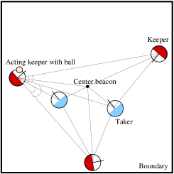
Figure 3: Illustrating keepaway. The various lines and angles indicate the 13 state variables making up each sensation as provided by the keepaway benchmark software.

5 Experiments

In this section we are finally ready to apply our proposed approach to the keepaway problem. We implemented and compared two different variations of the basic algorithm in a policy iteration based framework: (a) Optimistic policy iteration using LSPE($\lambda$) and (b) Actor-critic policy iteration using LSTD($\lambda$). As baseline method we used Sarsa($\lambda$) with tilecoding, which we re-implemented from (Stone et al., 2005) as faithfully as possible. Initially, we also tried to employ BRM instead of LSTD in the actor-critic framework. However, this set-up did not fare well in our experiments because of the stochastic state-transitions in keepaway (resulting in highly variable outcomes) and BRM’s inability to deal with this situation adequately. Thus, the results for BRM are not reported here.

Optimistic policy iteration.

Sarsa($\lambda$) and LSPE($\lambda$) paired with optimistic policy iteration is an on-policy learning method, meaning that the learning procedure estimates the Q-values from and for the current policy being executed by the agent. At the same time, the agent continually updates the policy according to the changing estimates of the Q-function. Thus policy evaluation and improvement are tightly interwoven. Optimistic policy iteration (OPI) is an online method that immediately processes the observed transitions as they become available from the agent interacting with the environment (Bertsekas and Tsitsiklis, 1996; Sutton and Barto, 1998).

Actor-critic.

In contrast, LSTD($\lambda$) paired with actor-critic is an off-policy learning method adhering with more rigor to the policy iteration framework. Here the learning procedure estimates the Q-values for a fixed policy, i.e. a policy that is not continually modified to reflect the changing estimates of Q. Instead, one collects a large number of state transitions under the same policy and estimates Q from these training examples. In OPI, where the most recent version of the Q-function is used to derive the next control action, only one network is required to represent Q and make the predictions. In contrast, the actor-critic framework maintains two instantiations of regularization networks: one (the actor) is used to represent the Q-function learned during the previous policy evaluation step and which is now used to represent the current policy, i.e. control actions are derived using its predictions. The second network (the critic) is used to represent the current Q-function and is updated regularly.

One advantage of the actor-critic approach is that we can reuse the same set of observed transitions to evaluate different policies, as proposed in (Lagoudakis and Parr, 2003). We maintain an ever-growing list of all transitions observed from the learning agent (irrespective of the policy), and use it to evaluate the current policy with LSTD($\lambda$). To reflect the real-time nature of learning in RoboCup, where we can only carry out a very small amount of computations during one single function call to the agent, we evaluate the transitions in small batches (20 examples per step). Once we have completed evaluating all training examples in the list, the critic network is copied to the actor network and we can proceed to the next iteration, starting anew to process the examples, using this time a new policy.

Policy improvement and $\varepsilon$-greedy action selection.

To carry out policy improvement, every time we need to determine a control action for an arbitrary state $s^{*}$, we choose the action $a^{*}$ that achieves the maximum Q-value; that is, given weights $\mathbf{w}_{k}$ and a set of basis functions $\{\mathbf{\tilde{x}}_{1},\ldots,\mathbf{\tilde{x}}_{m}\}$, we choose

$$a^{*}=\mathop{\mathrm{argmax}}_{a}\ \tilde{Q}(s^{*},a;\mathbf{w}_{k})=\mathop{\mathrm{argmax}}_{a}\ \mathbf{k}_{m}(s^{*},a)^{\text{T}}\mathbf{w}_{k}.$$

Sometimes however, instead of choosing the best (greedy) action, it is recommended to try out an alternative (non-greedy) action to ensure sufficient exploration. Here we employ the $\varepsilon$-greedy selection scheme; we choose a random action with a small probability $\varepsilon$ ( $\varepsilon=0.01$), otherwise we pick the greedy action with probability $1-\varepsilon$. Taking a random action usually means to choose among all possible actions with equal probability.

Under the standard assumption for errors in Bayesian regression (e.g., see Rasmussen and Williams, 2006), namely that the observed target values differ from the true function values by an additive noise term (i.i.d. Gaussian noise with zero mean and uniform variance), it is also possible to obtain an expression for the ‘predictive variance’ which measures the uncertainty associated with value predictions. The availability of such confidence intervals (which is possible for the direct least-squares problems LSPE and also BRM) could be used, as suggested in (Engel et al., 2005a), to guide the choice of actions during exploration and to increase the overall performance. For the purpose of solving the keepaway problem however, our initial experiments showed no measurable increase in performance when including this additional feature.

Remaining parameters.

Since the kernel is defined for state-action tuples, we employ a product kernel $k([s,a],[s^{\prime},a^{\prime}])=k_{S}(s,s^{\prime})k_{A}(a,a^{\prime})$ as suggested by Engel et al. (2005a). The action kernel $k_{A}(a,a^{\prime})$ is taken to be the Kronecker delta, since the actions in keepaway are discrete and disparate. As state kernel $k_{S}(s,s^{\prime})$ we chose the Gaussian RBF $k_{S}(s,s^{\prime})=\exp(-h\left\|{s-s^{\prime}}\right\|^{2})$ with uniform length-scale $h^{-1}=0.2$. The other parameters were set to: regularization $\sigma^{2}=0.1$, discount factor for RL $\gamma=0.99$, $\lambda=0.5$, and LSPE step size $\eta_{t}=0.5$. The novelty parameter for basis selection was set to $\texttt{TOL1}=0.1$. For the usefulness part we tried out different values to examine the effect supervised basis selection has; we started with $\texttt{TOL2}=0$ corresponding to the unsupervised case and then began increasing the tolerance, considering alternatively the settings $\texttt{TOL2}=0.001$ and $\texttt{TOL2}=0.01$. Since in the case of LSTD we are not directly solving a least-squares problem, we use the associated BRM formulation to obtain an expression for the error reduction in the supervised basis selection. Due to the very long runtime of the simulations (simulating one hour in the soccer server roughly takes one hour real time on a standard PC) we could not try out many different parameter combinations. The parameters governing RL were set according to our experiences with smaller problems and are in the range typically reported in the literature. The parameters governing the choice of the kernel (i.e. the length-scale of the Gaussian RBF) was chosen such that for the unsupervised case ($\texttt{TOL2}=0$) the number of selected basis functions approaches the maximum number of basis functions the CPU used for these the experiments was able to process in real-time. This number was determined to be $\sim 1400$ (on a standard 2 GHz PC).

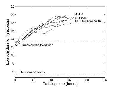
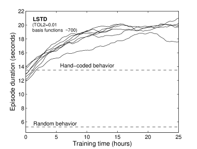
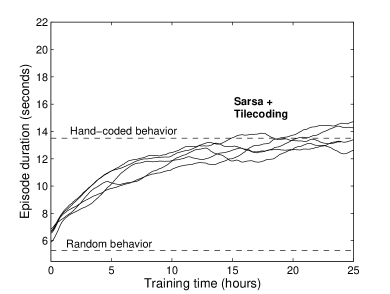
Figure 4: From left to right: Learning curves for our approach with LSTD (TOL2=0), LSTD (TOL2=0.001), LSTD (TOL2=0.01), and LSPE. At the bottom we show the curves for Sarsa with tilecoding corresponding to (Stone et al., 2005). We plot the average time the keepers are able to control the ball (quality of learned behavior) against the training time. After interacting for 15 hours the performance does not increase any more and the agent has experienced roughly 35,000 state transitions.

Results.

We evaluate every algorithm/parameter configuration using 5 independent runs. The learning curves for these runs are shown in Figure 4. The curves plot the average time the keepers are able to keep the ball (corresponding to the performance) against the simulated time the keepers were learning (roughly corresponding to the observed training examples). Additionally, two horizontal lines indicate the scores for the two benchmark policies random behavior and optimized hand-coded behavior used in (Stone et al., 2005).

The plots show that generally RL is able to learn policies that are at least as effective as the optimized hand-coded behavior. This is indeed quite an achievement, considering that the latter is the product of considerable manual effort. Comparing the three approaches Sarsa, LSPE and LSTD we find that the performance of LSPE is on par with Sarsa. The curves of LSTD tell a different story however; here we are outperforming Sarsa by 25% in terms of performance (in Sarsa the best performance is about $15$ seconds, in LSTD the best performance is about $20$ seconds). This gain is even more impressive when we consider the time scale at which this behavior is learned; just after a mere 2 hours we are already outperforming hand-coded control. Thus our approach needs far fewer state transitions to discover good behavior. The third observation shows the effectiveness of our proposed supervised basis function selection; here we show that our supervised approach performs as well as the unsupervised one, but requires significantly fewer basis functions to achieve that level of performance ($\sim$ 700 basis functions at TOL2$=0.01$ against 1400 basis functions at TOL2$=0$).

Regarding the unexpectedly weak performance of LSPE in comparison with LSTD, we conjecture that this strongly depends on the underlying architecture of policy iteration (i.e. OPI vs. actor-critic) as well as the specific learning problem. On a related number of experiments carried out with the octopus arm benchmark we made exactly the opposite observation (not discussed here in more detail, see Jung and Polani, 2007).

6 Discussion and related work

We have presented a kernel-based approach for least-squares based policy evaluation in RL using regularization networks as underlying function approximator. The key point is an efficient supervised basis selection mechanism, which is used to select a subset of relevant basis functions directly from the data stream. The proposed method was particularly devised with high-dimensional, stochastic control tasks for RL in mind; we prove its effectiveness using the RoboCup keepaway benchmark. Overall the results indicate that kernel-based online learning in RL is very well possible and recommendable. Even the rather few simulation runs we made clearly show that our approach is superior to convential function approximation in RL using grid-based tilecoding. What could be even more important is that the kernel-based approach only requires the setting of some fairly general parameters that do not depend on the specific control problem one wants to solve. On the other hand, using tilecoding or a fixed basis function network in high dimensions requires considerable manual effort on part of the programmer to carefully devise problem-specific features and manually choose suitable basis functions.

Engel et al. (2003, 2005a) initially advocated using kernel-based methods in RL and proposed the related GPTD algorithm. Our method using regularization networks develops this idea further. Both methods have in common the online selection of relevant basis functions based on (Csató and Opper, 2001). As opposed to the unsupervised selection in GPTD, we use a supervised criterion to further reduce the number of relevant basis functions selected. A more fundamental difference is the policy evaluation method addressed by the respective formulation; GPTD models the Bellman residuals and corresponds to the BRM approach (see Section 2.1.2). Thus, in its original formulation GPTD can be only applied to RL problems with deterministic state transitions. In contrast, we provide a unified and concise formulation of LSTD and LSPE which can deal with stochastic state transitions as well. Another difference is the type of benchmark problem used to showcase the respective method; GPTD was demonstrated by learning to control a simulated octopus arm, which was posed as an 88-dimensional control problem (Engel et al., 2005b). Controlling the octopus arm is a deterministic control problem with known state transitions and was solved there using model-based RL. In contrast, 3vs2 keepaway is only a 13-dimensional problem; here however, we have to deal with stochastic and unknown state transitions and need to use model-free RL.

Acknowledgments

The authors wish to thank the anonymous reviewers for their useful comments and suggestions.

A A summary of the updates

Let $\mathbf{x}_{t+1}=(s_{t+1},a_{t+1})$ be the next state-action tuple and $r_{t+1}$ be the reward assiociated with transition from the previous state $s_{t}$ to $s_{t+1}$ under $a_{t}$. Define the abbreviations:

$$\mathbf{k}_{t} :=\mathbf{k}_{m}(\mathbf{x}_{t}) \mathbf{k}_{t+1} :=\mathbf{k}_{m}(\mathbf{x}_{t+1}) \mathbf{h}_{t+1} :=\mathbf{k}_{t}-\gamma\mathbf{k}_{t+1}$$

$$k^{*}_{t} :=k(\mathbf{x}_{t},\mathbf{x}_{t+1}) k^{*}_{t+1} :=k(\mathbf{x}_{t+1},\mathbf{x}_{t+1}) h^{*}_{t+1} :=k^{*}_{t}-\gamma k^{*}_{t+1}$$

and $\mathbf{a}_{t+1}:=\mathbf{K}_{mm}^{-1}\mathbf{k}_{t+1}$.

A.1 Unsupervised basis selection

We want to test if $\mathbf{x}_{t+1}$ is well represented by the current basis functions in the dictionary or if we need to add $\mathbf{x}_{t+1}$ to the basis elements. Compute

$$\delta=k^{*}_{t+1}-\mathbf{k}_{t+1}^{\text{T}}\mathbf{a}_{t+1}.$$

If $\delta<\texttt{TOL1}$, then add $\mathbf{x}_{t+1}$ to the dictionary, execute the growing step (see below) and update

$$\mathbf{K}_{m+1,m+1}^{-1}=\begin{bmatrix}\mathbf{K}_{mm}^{-1}&\mathbf{0}\\ \mathbf{0}^{\text{T}}&0\end{bmatrix}+\frac{1}{\delta}\begin{bmatrix}-\mathbf{a}_{t+1}\\ 1\end{bmatrix}\begin{bmatrix}-\mathbf{a}_{t+1}\\ 1\end{bmatrix}^{\text{T}}.$$

A.2 Recursive updates for BRM

• Normal step $\{t,m\}\mapsto\{t+1,m\}$:

  1. $$\mathbf{P}_{t+1,m}^{-1}=\mathbf{P}_{tm}^{-1}-\frac{\mathbf{P}_{tm}^{-1}\mathbf{h}_{t+1}\mathbf{h}_{t+1}^{\text{T}}\mathbf{P}_{tm}^{-1}}{\Delta}$$

     with $\Delta=1+\mathbf{h}_{t+1}^{\text{T}}\mathbf{P}_{tm}^{-1}\mathbf{h}_{t+1}$.

  2. $$\mathbf{w}_{t+1,m}=\mathbf{w}_{tm}+\frac{\varrho}{\Delta}\mathbf{P}_{tm}^{-1}\mathbf{h}_{t+1}$$

     with $\varrho=r_{t+1}-\mathbf{h}_{t+1}^{\text{T}}\mathbf{w}_{tm}$.

• Growing step $\{t+1,m\}\mapsto\{t+1,m+1\}$

  1. $$\mathbf{P}_{t+1,m+1}^{-1}=\begin{bmatrix}\mathbf{P}_{t+1,m}^{-1}&\mathbf{0}\\ \mathbf{0}&0\end{bmatrix}+\frac{1}{\Delta_{b}}\begin{bmatrix}-\mathbf{w}_{b}\\ 1\end{bmatrix}\begin{bmatrix}-\mathbf{w}_{b}\\ 1\end{bmatrix}^{\text{T}}$$

     where

     $$\mathbf{w}_{b}=\mathbf{a}_{t+1}+\frac{\delta_{h}}{\Delta}\mathbf{P}_{tm}^{-1}\mathbf{h}_{t+1},\qquad\Delta_{b}=\frac{\delta_{h}^{2}}{\Delta}+\sigma^{2}\delta_{h},\qquad\delta_{h}=h^{*}_{t+1}-\mathbf{h}_{t+1}^{\text{T}}\mathbf{a}_{t+1}$$

  2. $$\mathbf{w}_{t+1,m+1}=\begin{bmatrix}\mathbf{w}_{t+1,m}\\ 0\end{bmatrix}+\kappa\begin{bmatrix}-\mathbf{w}_{b}\\ 1\end{bmatrix}$$

     where $\kappa=-\frac{\delta_{h}\varrho}{\Delta_{b}\Delta}$.

• Reduction of regularized cost when adding $\mathbf{x}_{t+1}$ (supervised basis selection):

  $$\xi_{t+1,m+1}=\xi_{t+1,m}-\kappa^{2}\Delta_{b}$$

  For supervised basis selection we additionally check if $\kappa^{2}\Delta_{b}>\texttt{TOL2}$.

A.3 Recursive updates for LSTD($\lambda$)

• Normal step $\{t,m\}\mapsto\{t+1,m\}$:

  1. $$\mathbf{z}_{t+1,m}=(\gamma\lambda)\mathbf{z}_{tm}+\mathbf{k}_{t}$$

  2. $$\mathbf{P}_{t+1,m}^{-1}=\mathbf{P}_{tm}^{-1}-\frac{\mathbf{P}_{tm}^{-1}\mathbf{z}_{t+1,m}\mathbf{h}_{t+1}^{\text{T}}\mathbf{P}_{tm}^{-1}}{\Delta}$$

     with $\Delta=1+\mathbf{h}_{t+1}^{\text{T}}\mathbf{P}_{tm}^{-1}\mathbf{z}_{t+1,m}$.

  3. $$\mathbf{w}_{t+1,m}=\mathbf{w}_{tm}+\frac{\varrho}{\Delta}\mathbf{P}_{tm}^{-1}\mathbf{z}_{t+1,m}$$

     with $\varrho=r_{t+1}-\mathbf{h}_{t+1}^{\text{T}}\mathbf{w}_{tm}$.

• Growing step $\{t+1,m\}\mapsto\{t+1,m+1\}$

  1. $$\mathbf{z}_{t+1,m+1}=\begin{bmatrix}\mathbf{z}_{t+1,m}^{\text{T}}&z_{t+1,m}^{*}\end{bmatrix}^{\text{T}}$$

     where $z_{t+1,m}^{*}=(\gamma\lambda)\mathbf{z}_{tm}^{\text{T}}\mathbf{a}_{t+1}+k^{*}_{t}$.

  2. $$\mathbf{P}_{t+1,m+1}^{-1}=\begin{bmatrix}\mathbf{P}_{t+1,m}^{-1}&\mathbf{0}\\ \mathbf{0}&0\end{bmatrix}+\frac{1}{\Delta_{b}}\begin{bmatrix}-\mathbf{w}_{b}^{(1)}\\ 1\end{bmatrix}\begin{bmatrix}-\mathbf{w}_{b}^{(2)}&1\end{bmatrix}$$

     where

     $$\mathbf{w}_{b}^{(1)} =\mathbf{a}_{t+1}+\frac{\delta^{(1)}}{\Delta}\mathbf{P}_{tm}^{-1}\mathbf{z}_{t+1,m} \delta^{(1)} =h^{*}_{t+1}-\mathbf{a}_{t+1}^{\text{T}}\mathbf{h}_{t+1}$$

     $$\mathbf{w}_{b}^{(2)} =\mathbf{a}_{t+1}^{\text{T}}+\frac{\delta^{(2)}}{\Delta}\mathbf{h}_{t+1}^{\text{T}}\mathbf{P}_{tm}^{-1} \delta^{(2)} =z_{t+1,m}^{*}-\mathbf{a}_{t+1}^{\text{T}}\mathbf{z}_{t+1,m}$$

     and $\Delta_{b}=\frac{\delta^{(1)}\delta^{(2)}}{\Delta}+\sigma^{2}(k^{*}_{t+1}-\mathbf{k}_{t+1}^{\text{T}}\mathbf{a}_{t+1})$.

  3. $$\mathbf{w}_{t+1,m+1}=\begin{bmatrix}\mathbf{w}_{t+1,m}\\ 0\end{bmatrix}+\kappa\begin{bmatrix}-\mathbf{w}_{b}^{(1)}\\ 1\end{bmatrix}$$

     where $\kappa=-\frac{\delta^{(2)}\varrho}{\Delta_{b}\Delta}$.

A.4 Recursive updates for LSPE($\lambda$)

• Normal step $\{t,m\}\mapsto\{t+1,m\}$:

  1. $$\mathbf{z}_{t+1,m} = (\gamma\lambda)\mathbf{z}_{tm}+\mathbf{k}_{t+1}$$

     $$\mathbf{A}_{t+1,m} = \mathbf{A}_{tm}+\mathbf{z}_{t+1,m}\mathbf{h}_{t+1}^{\text{T}}$$

     $$\mathbf{b}_{t+1,m} = \mathbf{b}_{tm}+\mathbf{z}_{t+1,m}r_{t+1}$$

  2. $$\mathbf{P}_{t+1,m}^{-1}=\mathbf{P}_{tm}^{-1}-\frac{\mathbf{P}_{tm}^{-1}\mathbf{k}_{t+1}\mathbf{k}_{t+1}^{\text{T}}\mathbf{P}_{tm}^{-1}}{\Delta}$$

     with $\Delta=1+\mathbf{k}_{t+1}^{\text{T}}\mathbf{P}_{tm}^{-1}\mathbf{k}_{t+1}$.

  3. $$\mathbf{w}_{t+1,m}=\mathbf{w}_{tm}+\eta\mathbf{P}_{t+1,m}^{-1}(\mathbf{b}_{t+1,m}-\mathbf{A}_{t+1,m}\mathbf{w}_{tm})$$

• Growing step $\{t+1,m\}\mapsto\{t+1,m+1\}$

  1. $$\mathbf{z}_{t+1,m+1}=\begin{bmatrix}\mathbf{z}_{t+1,m}\\ z_{t+1,m}^{*}\end{bmatrix}\qquad\qquad\mathbf{b}_{t+1,m+1}=\begin{bmatrix}\mathbf{b}_{t+1,m}\\ \mathbf{a}_{t+1}^{\text{T}}\mathbf{b}_{tm}+z_{t+1,m}^{*}r_{t+1}\end{bmatrix}$$

     $$\mathbf{A}_{t+1,m+1}=\begin{bmatrix}\mathbf{A}_{t+1,m}&\mathbf{A}_{tm}\mathbf{a}_{t+1}+\mathbf{z}_{t+1,m}h^{*}\\ \mathbf{a}_{t+1}^{\text{T}}\mathbf{A}_{tm}+z_{t+1,m}^{*}\mathbf{h}_{t+1}^{\text{T}}&\mathbf{a}_{t+1}^{\text{T}}\mathbf{A}_{tm}\mathbf{a}_{t+1}+z_{t+1,m}^{*}h^{*}\end{bmatrix}$$

     where $z_{t+1,m}^{*}=(\gamma\lambda)\mathbf{z}_{tm}^{\text{T}}\mathbf{a}_{t+1}+k^{*}_{t}$.

  2. $$\mathbf{P}_{t+1,m+1}^{-1}=\begin{bmatrix}\mathbf{P}_{t+1,m}^{-1}&\mathbf{0}\\ \mathbf{0}&0\end{bmatrix}+\frac{1}{\Delta_{b}}\begin{bmatrix}-\mathbf{w}_{b}\\ 1\end{bmatrix}\begin{bmatrix}-\mathbf{w}_{b}\\ 1\end{bmatrix}^{\text{T}}$$

     where

     $$\mathbf{w}_{b}=\mathbf{a}_{t+1}+\frac{\delta}{\Delta}\mathbf{P}_{tm}^{-1}\mathbf{k}_{t+1},\qquad\Delta_{b}=\frac{\delta^{2}}{\Delta}+\sigma^{2}\delta,\qquad\delta=k^{*}_{t}-\mathbf{k}_{t}^{\text{T}}\mathbf{a}_{t+1}$$

     and $\Delta_{b}=\frac{\delta^{(1)}\delta^{(2)}}{\Delta}+\sigma^{2}(k^{*}_{t+1}-\mathbf{k}_{t+1}^{\text{T}}\mathbf{a}_{t+1})$.

  3. $$\mathbf{w}_{t+1,m+1}=\begin{bmatrix}\mathbf{w}_{t+1,m}\\ 0\end{bmatrix}+\kappa\begin{bmatrix}-\mathbf{w}_{b}^{(1)}\\ 1\end{bmatrix}$$

     where $\kappa=-\frac{\delta^{(2)}\varrho}{\Delta_{b}\Delta}$.

• Reduction of regularized cost when adding $\mathbf{x}_{t+1}$ (supervised basis selection):

  $$\xi_{t+1,m+1}=\xi_{t+1,m}-\Delta_{b}^{-1}(c-\mathbf{w}_{b}^{\text{T}}\mathbf{d})^{2}$$

  where $c=\mathbf{a}_{t+1}^{\text{T}}(\mathbf{b}_{tm}-\mathbf{A}_{tm}\mathbf{w}_{tm})+z^{*}_{t+1,m}(r_{t+1}-\mathbf{h}_{t+1}^{\text{T}}\mathbf{w}_{tm})$ and $\mathbf{d}=\mathbf{b}_{t+1,m}-\mathbf{A}_{t+1,m}\mathbf{w}_{tm}$. For supervised basis selection we additionally check if $\Delta_{b}^{-1}(c-\mathbf{w}_{b}^{\text{T}}\mathbf{d})^{2}>\texttt{TOL2}$.

References

- Baird [1995] L. C. Baird. Residual algorithms: Reinforcement learning with function approximation. In Proc. of ICML 12, pages 30–37, 1995.
- Bertsekas and Tsitsiklis [1996] D. Bertsekas and J. Tsitsiklis. Neuro-dynamic programming. Athena Scientific, 1996.
- Bertsekas et al. [2004] D. P. Bertsekas, V. S. Borkar, and A. Nedić. Improved temporal difference methods with linear function approximation. In A. Barto, W. Powell, and J. Si, editors, Learning and Approximate Dynamic Programming. IEEE Press, 2004.
- Bertsekas and Ioffe [1996] D. P. Bertsekas and S. Ioffe. Temporal differences-based policy iteration and applications in neuro-dynamic programming. LIDS Tech. Report LIDS-P-2349, MIT, 1996.
- Boyan [1999] J. A. Boyan. Least-squares temporal difference learning. In Proc. of ICML 16, pages 49–56, 1999.
- Bradtke and Barto [1996] S. J. Bradtke and A. Barto. Linear least-squares algorithms for temporal difference learning. Machine Learning, 22:33–57, 1996.
- Csató and Opper [2001] L. Csató and M. Opper. Sparse representation for Gaussian process models. In Advances in NIPS 13, pages 444–450, 2001.
- Engel et al. [2003] Y. Engel, S. Mannor, and R. Meir. Bayes meets Bellman: The Gaussian process approach to temporal difference learning. In Proc. of ICML 20, pages 154–161, 2003.
- Engel et al. [2005a] Y. Engel, S. Mannor, and R. Meir. Reinforcement learning with Gaussian processes. In Proc. of ICML 22, 2005a.
- Engel et al. [2005b] Y. Engel, P. Szabo, and D. Volkinshtein. Learning to control an octopus arm with Gaussian process temporal difference methods. In Advances in NIPS 17, 2005b.
- Fine and Scheinberg [2001] S. Fine and K. Scheinberg. Efficient SVM training using low-rank kernel representation. JMLR, 2:243–264, 2001.
- Girosi et al. [1995] F. Girosi, M. Jones, and T. Poggio. Regularization theory and neural networks architectures. Neural Computation, 7:219–269, 1995.
- Jung and Polani [2006] T. Jung and D. Polani. Sequential learning with LS-SVM for large-scale data sets. In Proc. of ICANN 16, pages 381–390, 2006.
- Jung and Polani [2007] T. Jung and D. Polani. Kernelizing LSPE(). In Proc. of IEEE Symposium on Approximate Dynamic Programming and Reinforcement Learning, 2007.
- Lagoudakis and Parr [2003] M. G. Lagoudakis and R. Parr. Least-squares policy iteration. JMLR, 4:1107–1149, 2003.
- Luo and Wahba [1997] Z. Luo and G. Wahba. Hybrid adaptive splines. J. Amer. Statist. Assoc., 92:107–116, 1997.
- Nedić and Bertsekas [2003] A. Nedić and D. P. Bertsekas. Least squares policy evaluation algorithms with linear function approximation. Discrete Event Dynamic Systems: Theory and Applications, 13:79–110, 2003.
- Noda et al. [1998] I. Noda, H. Matsubara, K. Hiraki, and I. Frank. Soccer server: A tool for research on multiagent systems. Applied Artificial Intelligence, 12:233–250, 1998.
- Poggio and Girosi [1990] T. Poggio and F. Girosi. Networks for approximation and learning. Proceedings of the IEEE, 78(9):1481–1497, 1990.
- Rasmussen and Quiñonero Candela [2005] C. E. Rasmussen and J. Quiñonero Candela. Healing the relevance vector machine through augmentation. In Proc. of ICML 22, pages 689–696, 2005.
- Rasmussen and Williams [2006] C. E. Rasmussen and C. K. I. Williams. Gaussian Processes for Machine Learning. MIT Press, 2006.
- Sayed [2003] A. Sayed. Fundamentals of Adaptive Filtering. Wiley Interscience, 2003.
- Smola and Bartlett [2001] A. J. Smola and P. L. Bartlett. Sparse greedy Gaussian process regression. In Advances in NIPS 13, pages 619–625, 2001.
- Smola and Schölkopf [2000] A. J. Smola and B. Schölkopf. Sparse greedy matrix approximation for machine learning. In Proc. of ICML 17, pages 911–918, 2000.
- Stone et al. [2005] P. Stone, R. S. Sutton, and G. Kuhlmann. Reinforcement learning for RoboCup-soccer keepaway. Adaptive Behavior, 13(3):165–188, 2005.
- Sutton and Barto [1998] R. Sutton and A. Barto. Reinforcement Learning: An Introduction. MIT Press, 1998.
- Sutton [1988] R. S. Sutton. Learning to predict by the methods of temporal differences. Machine Learning, 3:9–44, 1988.
- Tsitsiklis and Roy [1997] J. N. Tsitsiklis and B. Van Roy. An analysis of temporal difference learning with function approximation. IEEE Transactions on Automatic Control, 42(5):674–690, 1997.
- Wahba [1990] G. Wahba. Spline models for observational data. Series in Applied Mathematics, Philadelphia, Vol. 59. SIAM, 1990.
- Williams and Seeger [2001] C. Williams and M. Seeger. Using the Nyström method to speed up kernel machines. In Advances in NIPS 13, pages 682–688, 2001.