Fluctuation-dissipation relation for chaotic non-Hamiltonian systems

Abstract

In dissipative dynamical systems phase space volumes contract, on average. Therefore, the invariant measure on the attractor is singular with respect to the Lebesgue measure. As noted by Ruelle, a generic perturbation pushes the state out of the attractor, hence the statistical features of the perturbation and, in particular, of the relaxation, cannot be understood solely in terms of the unperturbed dynamics on the attractor. This remark seems to seriously limit the applicability of the standard fluctuation dissipation procedure in the statistical mechanics of nonequilibrium (dissipative) systems. In this paper we show that the singular character of the steady state does not constitute a serious limitation in the case of systems with many degrees of freedom. The reason is that one typically deals with projected dynamics, and these are associated with regular probability distributions in the corresponding lower dimensional spaces.

1 Introduction

Since its early developments, due mainly to the works of L. Onsager and R. Kubo [1, 2, 3, 4], the fluctuation-dissipation theorem (FDT) represents a cornerstone in the construction of a theory of nonequilibrium phenomena [5]. This celebrated result was developed in the context of Hamiltonian dynamical systems, slightly perturbed out of their thermodynamic equilibrium, and it was later extended to stochastic systems obeying a Langevin Equation [6, 7]. The importance of the FDT rests on the fact that it sheds light on the crucial relation between the response $R_{V}(t)$ of a system to an external perturbation and a time correlation function computed at equilibrium. In other words, having perturbed a given Hamiltonian $H_{0}$ with an external field $h_{e}$, to obtain the perturbed Hamiltonian $H_{0}-h_{e}V$, where $V$ is an observable conjugated with $h_{e}$, the FDT allows us to compute nonequilibrium quantities, such as the transport coefficients [8, 9], solely in terms of the unperturbed equilibrium state. On the other hand, a generic dynamical system is not Hamiltonian: for phenomenological practical pruposes, one typically deals with dissipative dynamics, as in the important case of viscous hydrodynamics [6].

The invariant measure of a chaotic dissipative system, $\mu$ say, is singular with respect to the Lebesgue measure and is usually supported on a fractal attractor. This is not just a mathematical curiosity, it is a potential source of difficulties for the applicability of the FDT in dissipative systems. Indeed, the standard FDT ensures that the statistical features of a perturbation are related to the statistical properties of the unperturbed system, but that cannot be the case in general, in dissipative systems. The reason is that, given an initial state $\underline{x}(0)$ on the attractor and a generic perturbation $\delta\underline{x}(0)$, the perturbed initial state $\underline{x}^{(p)}(0)=\underline{x}(0)+\delta\underline{x}(0)$ and its time evolution may lie outside the support of $\mu$, hence their statistical properties cannot be expressed by $\mu$, which attributes vanishing probability to such states. In the cases considered by Ruelle [10], the perturbation $\delta\underline{x}(0)$ and its time evolution $\delta\underline{x}(t)$ can be decomposed as the sum of two parts, $\delta\underline{x}_{\perp}(t)$ and $\delta\underline{x}_{\parallel}(t)$, respectively perpendicular and parallel to the “fibres” of the attractor,

$$\delta\underline{x}(t)=\delta\underline{x}_{\perp}(t)+\delta\underline{x}_{\parallel}(t)$$

which makes it natural to expect that the statistical features of $\delta\underline{x}_{\parallel}(t)$ be related to the dynamics on the attractor, while it is easy to construct examples in which $\delta\underline{x}_{\perp}(t)$ is not described by the unperturbed dynamics.

From the mathematical point of view, this fact is rather transparent. On the other hand, it should not be a concern in statistical mechanics, except in pathological cases. Indeed, a series of numerical investigations of chaotic dissipative systems shows that the standard FDT holds under rather general conditions, mainly if the invariant measure is absolutely continuous with respect to Lebesgue, cf. Ref.[6] for a review. Moreover, although dissipative systems have singular invariant measures, any small amount of noise produces smooth invariant measures, which allow generalized FDTs to be expressed solely in terms of the unperturbed states, analogously to the standard equilibrium case. Apart from technical aspects, the intuitive reason for which the FDT in systems with noise can be expressed only in terms of the invariant measure, is that $\underline{x}^{p}(0)$ remains within the support of this measure.

In this paper, we want to take advantage of the fact that a similar situation is realized without any noise, if one works in the projected space of the physically relevant observables. Indeed, marginals of singular phase space measures, on spaces of sufficiently lower dimension than the phase space, are usually regular [11, 12].

Our paper is organized as follows: Section 2 is devoted to a short presentation of some general results on FDT for chaotic dissipative systems. In Sec. 3 we discuss the numerical results for two dissipative chaotic maps, showing that the singular character of their invariant measures does not prevent the response of standard observables to be expressed only in terms of the invariant measure, as in the standard case. Conclusions are drawn in Sec. 4.

2 Some results on FDT in chaotic dissipative systems

Let us concisely recall Ruelle’s approach to linear response in deterministic dissipative dynamical systems [10]. Let ($\mathcal{M},S^{t},\mu$) be a dynamical system, with $\mathcal{M}$ its compact phase space, $S^{t}:\mathcal{M}\rightarrow\mathcal{M}$ a one parameter group of diffeomorphisms and $\mu$ the invariant natural measure. Following Ruelle [10], who considers axiom A systems, one may show that the effect of a perturbation $\delta F(t)=\delta F_{\parallel}(t)+\delta F_{\perp}(t)$ on the response of a generic (smooth enough) observable $A$ attains the form:

$$\delta\overline{A}(t)=\int_{0}^{t}R_{\parallel}^{(A)}(t-\tau)\delta F_{\parallel}(\tau)d\tau+\int_{0}^{t}R_{\perp}^{(A)}(t-\tau)\delta F_{\perp}(\tau)d\tau$$ (1)

where the subscript _∥ refers to the dynamics on the unstable tangent bundle (along the attractor), while _⟂ refers to the transversal directions, cf. left panel of Fig. 1. Ruelle’s central remark is that $R_{\parallel}^{(A)}$ may be expressed in terms of a correlation function evaluated with respect to the unperturbed dynamics, while $R_{\perp}^{(A)}$ depends on the dynamics along the stable manifold, hence it may not be determined by $\mu$, and should be quite difficult to compute numerically [6].

To illustrate these facts, the Authors of Ref.[13] study a $2$-dimensional model, which consists of a chaotic rotator on a plane and, for such a system, succeed to numerically estimate the $R_{\perp}^{(A)}$ term in eq.(1). Nevertheless, in the next Section, we argue that $R_{\perp}^{(A)}$ may spoil the generalized FDT only if the perturbation is carefully oriented with respect to the stable and unstable manifolds. This is only possible in peculiar situations, such as those of Ref.[13], in which the invariant measure is the product of a radial and and angular component and, furthermore, the perturbation lies on the radial direction, leaving the angular dynamics unaffected.

  

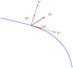
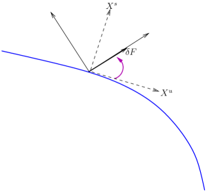
Figure 1: Left panel: In Ruelle’s approach, the perturbation is expressed as the sum of one component parallel to the unstable manifold and one parallel to the stable manifold. Right panel: In the present work, the reference frame is rotated so that the direction of the perturbation coincides with one of the basis vectors.

A different approach to the FDT has been proposed in [14], which concerns deterministic dynamics perturbed by stochastic contributions. Here, the invariant measure $\mu$ can be assumed to have density $\rho$: ${\rm d}\mu(\underline{x})=\rho(\underline{x})d\underline{x}$. Then, if the initial conditions are modified by an impulsive perturbation $\underline{x}_{0}\rightarrow\underline{x}_{0}+\delta\underline{x}_{0}$, the invariant density $\rho(\underline{x}_{0})$ is replaced by a perturbed initial density $\rho_{0}(\underline{x}_{0};\delta\underline{x}_{0})=\rho(\underline{x}_{0}-\delta\underline{x}_{0})$, where the subscript 0 denotes the initial state, right after the perturbation. This state is not stationary and evolves in time, producing time dependent densities $\rho_{t}(\underline{x}_{0};\delta\underline{x}_{0})$, which are assumed to eventually relax back to $\rho(\underline{x}_{0})$. Given the transition probability $W(\underline{x}_{0},0\rightarrow\underline{x},t)$ determined by the dynamics, the response of coordinate $x_{i}$ is expressed by:

$$\overline{\delta x_{i}(t)}=\int\int x_{i}\left[\rho(\underline{x}_{0}-\delta\underline{x}_{0})-\rho(\underline{x}_{0})\right]W(\underline{x}_{0},0\rightarrow\underline{x},t)d\underline{x}_{0}d\underline{x}$$ (2)

and one may introduce the response function $R_{ij}$ as [14]:

$$R_{ij}(t)=\frac{\overline{\delta x_{i}(t)}}{\delta x_{j}(0)}=-\left\langle x_{i}(t)\left.\frac{\partial\log\rho}{\partial x_{j}}\right|_{t=0}\right\rangle$$ (3)

which is a correlation function computed with respect to the unperturbed state. It is worth to note that it makes no difference in the derivation of eq.(3) whether the steady state is an equilibrium state or not; it suffices that $\rho$ be differentiable.

Let us consider again Eq.(2) and, for sake of simplicity, assume that all components of $\delta\underline{x}(0)$ vanish, except the $i$-th component. Then, the response of $x_{i}$ may also be written as:

$$\overline{\delta x_{i}}(t) = \int x_{i}\left\{\int\left[\rho(\underline{x}_{0}-\delta\underline{x}_{0})-\rho(\underline{x}_{0})\right]W(\underline{x}_{0},0\rightarrow\underline{x},t)d\underline{x}_{0}\prod_{j\neq i}dx_{j}\right\}dx_{i}$$ (4)

$$\equiv \int x_{i}B_{i}(x_{i},\delta\underline{x}_{0},t)dx_{i}$$

where $B_{i}(x_{i},\delta\underline{x}_{0},t)$, defined by the term within curly brackets, may also be written as:

$$B_{i}(x_{i},\delta\underline{x}_{0},t)=\widetilde{\rho_{t}}(x_{i};\delta\underline{x}_{0})-\widetilde{\rho}(x_{i})$$ (5)

where $\widetilde{\rho}(x_{i})$ and $\widetilde{\rho_{t}}$ are the marginal probability distributions defined by:

$$\widetilde{\rho}(x_{i})=\int\rho(\underline{x})\prod_{j\neq i}dx_{j}~{},\qquad\widetilde{\rho_{t}}(x_{i};\delta\underline{x}_{0})=\int\rho_{t}(\underline{x};\delta\underline{x}_{0})\prod_{j\neq i}dx_{j}~{}.$$

As projected singular measures are expected to be smooth, especially if the dimension of the projected space is sensibly smaller than that of the original space, one may adopt the same procedure also for dissipative deterministic dynamical systems. Indeed, the response function $B_{i}(x_{i},\delta\underline{x}_{0},t)$ in Eq.(5) is also expected to be smooth, and to make the response of $x_{i}$ computable from the invariant measure only. In the next section we investigate this possibility.

3 Coarse graining analysis

In terms of phase space probability measures, the response formula Eq.(2) reads:

$$\overline{\delta x_{i}}(t)=\int x_{i}~{}{\rm d}\mu_{t}(\underline{x};\delta\underline{x}_{0})-\int x_{i}~{}{\rm d}\mu(\underline{x})$$ (6)

where ${\rm d}\mu_{t}(\underline{x};\delta\underline{x}_{0})$ is the time evolving perturbed measure whose initial state is given by

$${\rm d}\mu_{0}(\underline{x}_{0};\delta\underline{x}_{0})=\rho_{0}(\underline{x}_{0};\delta\underline{x}_{0})~{}{\rm d}\underline{x}_{0}=\rho(\underline{x}_{0}-\delta\underline{x}_{0})~{}{\rm d}\underline{x}_{0}~{}.$$

Because dissipative dynamical systems do not have an invariant probability density, it is convenient to introduce a coarse graining in phase space, to approximate the singular invariant measure $\mu$ by means of piecewise constant distributions.

Let us consider a $d$-dimensional phase space $\mathcal{M}$, with an $\epsilon$-partition made of a finite set of $d$-dimensional hypercubes $\Lambda_{k}(\epsilon)$ of side $\epsilon$ and centers $\underline{x}_{k}$. Introduce the $\epsilon$-coarse graining of $\mu$ and of $\mu_{t}$ defined by the probabilities $P_{k}(\epsilon)$ and $P_{t,k}(\epsilon;\delta\underline{x}_{0})$ of the hypercubes $\Lambda_{k}(\epsilon)$:

$$P_{k}(\epsilon)=\int_{\Lambda_{k}(\epsilon)}{\rm d}\mu(\underline{x})\hskip 3.0pt,\quad P_{t,k}(\epsilon;\delta\underline{x}_{0})=\int_{\Lambda_{k}(\epsilon)}{\rm d}\mu_{t}(\underline{x};\delta\underline{x}_{0})~{}.$$ (7)

This leads to the coarse grained invariant density $\rho(\underline{x};\epsilon)$:

$$\rho(\underline{x};\epsilon)=\sum_{k}\rho_{k}(\underline{x};\epsilon)\hskip 3.0pt,\hskip 6.0pt\hbox{with}\hskip 6.0pt\rho_{k}(\underline{x};\epsilon)=\left\{\begin{array}[]{ll}P_{k}(\epsilon)/\epsilon^{d}&\hbox{if $x\in\Lambda_{k}(\epsilon)$}\\ 0&\hbox{else}\end{array}\right.$$ (8)

Let $Z_{i}$ be the number of bins of of form $\left[x_{i}^{(q)}-\epsilon/2,x_{i}^{(q)}+\epsilon/2\right)$, $q\in\{1,2,...,Z_{i}\}$, in the $i$-th direction. Then, the marginalization of the coarse grained distribution yields the following set of $Z_{i}$ probabilities:

$$\hskip-45.0ptp_{i}^{(q)}(\epsilon)=\int_{x_{i}^{(q)}-\frac{\epsilon}{2}}^{x_{i}^{(q)}+\frac{\epsilon}{2}}\left\{\int\rho(\underline{x};\epsilon)\prod_{j\neq i}dx_{j}\right\}{\rm d}x_{i}={\rm Prob}\left(x_{i}\in\left[x_{i}^{(q)}-\frac{\epsilon}{2},x_{i}^{(q)}+\frac{\epsilon}{2}\right)\right)$$ (9)

each of which is the invariant probability that the coordinate $x_{i}$ lie in one of the $Z_{i}$ bins. In an analogous way, one may define the marginal of the evolving coarse grained perturbed probability $p_{t,i}^{(q)}(\epsilon;\delta\underline{x}_{0})$. In both cases, dividing by $\epsilon$, one obtains the coarse grained marginal probability densities $\rho_{i}^{(q)}(\epsilon)$ and $\rho_{t,i}^{(q)}(\epsilon;\delta\underline{x}_{0})$, as well as the $\epsilon$-coarse grained version of the response function $B_{i}(x_{i},\delta\underline{x}_{0},t)$:

$$B_{i}^{(q)}(x_{i},\delta\underline{x}_{0},t,\epsilon)=\frac{1}{\epsilon}\left[p_{t,i}^{(q)}(\epsilon,\delta\underline{x}_{0})-p_{i}^{(q)}(\epsilon)\right]={\rho_{t,i}^{(q)}(\epsilon,\delta\underline{x}_{0})-\rho_{i}^{(q)}(\epsilon)}$$ (10)

In the following, we will show that the r.h.s. of Eq.(10) tends to a regular function of $x_{i}$ in the $Z_{i}\rightarrow\infty$, $\epsilon\to 0$, limit. Then, in the limit of small perturbations $\delta\underline{x}_{0}$, $B_{i}^{(q)}(x_{i},\delta\underline{x}_{0},t,\epsilon)$ may be expanded as a Taylor series, to yield an expression similar to standard response theory, in the sense that it depends solely on the unperturbed state. The difference, here, is that the invariant measure is singular and represents a nonequilibrium steady state.

To illustrate this fact, we run a set of $N$ trajectories with uniformly distributed initial conditions in the phase spaces of two simple, but substantially different, 2-dimensional maps: a dissipative baker map, and the Henon map.

3.1 The dissipative baker map

Let $\mathcal{M}=[0,1]\times[0,1]$ be the phase space, and consider the evolution equation

$$\left(\begin{array}[]{c}x_{n+1}\\ y_{n+1}\end{array}\right)=M\left(\begin{array}[]{c}x_{n}\\ y_{n}\end{array}\right)=\left\{\begin{array}[]{ll}\left(\begin{array}[]{c}x_{n}/l\\ ry_{n}\end{array}\right),&\hbox{for $0\leq x_{n}<l$;}\\ \left(\begin{array}[]{c}(x_{n}-l)/r\\ r+ly_{n}\end{array}\right),&\hbox{for $l\leq x_{n}\leq 1$.}\end{array}\right.\quad.$$ (11)

whose Jacobian determinant is given by

$$J_{M}(\underline{x})=\left\{\begin{array}[]{ll}J_{A}=r/l~{},&\hbox{for $\>0\leq x\leq l$;}\\ J_{B}=l/r=J_{A}^{-1}~{},&\hbox{for $\>l\leq x\leq 1$.}\end{array}\right.\quad.$$ (12)

and shows that the $M$ is dissiaptive for $l<1/2$. The map $M$ is hyperbolic, since stable and unstable manifolds which intersect each other orthogonally are defined at all points $\underline{x}\in\mathcal{M}$, except in the irrelevant vertical segment at $x=l$. The directions of these manifolds coincide, respectively, with the vertical and horizontal directions. It can also be shown that this dynamical system is endowed with an invariant measure $\mu$ which is smooth along the unstable manifold and singular along the stable one, cf. Figs.2. In particular, $\mu$ factorizes as ${\rm d}\mu(\underline{x})={\rm d}{x}\times{\rm d}\lambda(y)$, similarly to the case of [13].

In order to verify whether the functions corresponding to the above introduced $B_{i}^{(q)}(x_{i},\delta\underline{x}_{0},t,\epsilon)$ become regular functions in the fine graining limit, let us consider first an impulsive perturbation, directed purely along the stable manifold, i.e. $\delta\underline{x}_{0}=(0,\delta y_{0})$.

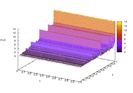
Figure 2: Invariant probability distribution of the map defined by Eq. (11).

Ruelle’s work on singular measures is clearly relevant, in this case, because the support of the marginal perturbed probability measure, obtained projecting out the $y$-direction has simply drifted preserving its singular character, while the state may have fallen outside the support of the unperturbed invariant measure, cf. left panel of Fig.3.

Consider now an initial impulsive perturbation with one component, no matter how small, along the unstable manifold, $\delta\underline{x}_{0}=(\delta x_{0},\delta y_{0})$ and rotate the vectors of the basis of the 2-dimensional plane, so that the coordinate $x$ lies along the direction of the perturbation, as shown in the right panel of Fig.1. We find that $B_{x}^{(q)}(x,\delta\underline{x}_{0},t,\epsilon)$ is regular as a function of $x$. Indeed, the projections of $\mu$ and of its perturbations onto the direction of $\delta\underline{x}_{0}$ have a density along all directions except the vertical one, cf. right panel of Fig.3. Hence, a small perturbation does not take the state outside the corresponding projected support.

As already noted in [13], this Baker map shows that the response to very carefully selected perturbations, cannot be computed in general from solely the invariant measure. However, similarly to the case of [13], the factorization of $\mu$ makes the present case rather peculiar. Indeed, for the overwhelming majority of dynamical systems, it looks impossible to select directions such that the projected measures preserve the same degree of singularity as the full measures. This is a consequence of the fact that stable and unstable manifolds have different orientations in different parts of the phase space, provided they exist. Clearly, the higher the dimensionality of the phase space and the larger the number of projected out dimensions, the more difficult it is to preserve singular characters.

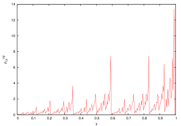
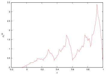
Figure 3: Left panel: singular distribution of the unperturbed system, obtained projecting the invariant measure onto the vertical direction $y$, which is the direction of the stable manifold. Right panel: projected invariant density along the direction of the perturbation, which forms an angle $\alpha=\pi/8$ radiants with the $y$-direction. $z=1-(x\cos(\alpha)-y\sin(\alpha)+\sin(\alpha))$ is the coordinate along this direction. Although hardly differentiable, this projected distribution has a density.

3.2 The Henon map

Consider for instance the Henon map defined by:

$$\left(\begin{array}[]{c}x_{n+1}\\ y_{n+1}\end{array}\right)=M\left(\begin{array}[]{c}x_{n}\\ y_{n}\end{array}\right)=\left(\begin{array}[]{c}y_{n}+1-ax_{n}^{2}\\ bx_{n}\end{array}\right).\quad$$ (13)

one the phase space $\mathcal{M}=[-\frac{3}{2},\frac{3}{2}]\times[\frac{1}{2},\frac{1}{2}]$, where $a=1.4$ and $b=0.3$ imply a chaotic dissipative dynamics, with a fractal invariant measure $\mu$, which is not the product of the marginal measures obtained by projecting onto the horizontal and the vertical directions. These marginals are indeed regular and would yield a regular product. As stable and unstable manifolds wind around, changing orientation, in a very complicated fashion, it seems impossible, here, to disentangle the contributions of one phase space direction from the other.

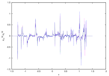
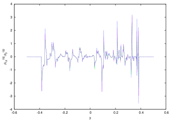
Figure 4: Left panel: plot of the function $B_{x}^{(q)}(x,\delta\underline{x}_{0},t,\epsilon)$, introduced by Eq.(5), for the Henon map, after $t=2$ iterations, with an initial perturbation along the $x$ direction, $\delta\underline{x}_{0}=(2.5\cdot 10^{-2},0)$, and different numbers of bins $Z_{x}$ on the $x$-axis, as well as different number $N$ of trajectories, so to keep the statistics in the $\epsilon\rightarrow 0$ limit: $N=3\cdot 10^{6},~{}Z_{x}=1320$ (green curve), $N=5\cdot 10^{6},~{}Z_{x}=1650$ (purple curve), $N=8\cdot 10^{6},~{}Z_{x}=1980$ (blue curve). Right panel: plot of the function $B_{y}^{(q)}(y,\delta\underline{x}_{0},t,\epsilon)$ after $t=2$ iterations, for the same initial perturbation considered in the left panel, and different values of bins $Z_{y}$ on the $y$-axis and different values of $N$: $N=3\cdot 10^{6},~{}Z_{y}=336$ (green curve), $N=5\cdot 10^{6},~{}Z_{y}=420$ (purple curve), $N=8\cdot 10^{6},~{}Z_{y}=505$ (blue curve). The curves largely overlap, but the figure does not clarify whether $B_{x}^{(q)},~{}B_{y}^{(q)}$ get smoother as $Z_{x}$ and $Z_{y}$ increase with $N$.

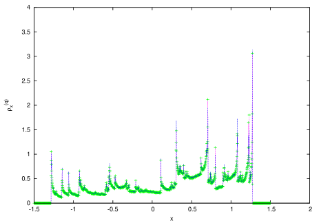
Figure 5: Plot of the projected invariant probability density $\rho_{x}^{(q)}(\epsilon)$, for the Henon map, with $N=5\cdot 10^{6}$, $Z_{x}=1650$ (purple curve, with green errorbars) and $N=8\cdot 10^{6}$, $Z_{x}=1980$ (blue curve). The figure does not clarify whether the invariant distribution is siungular or not.

Then, because no direction appears to be priviledged in phase space, an initial perturbation along one of the axis should not lead to any singular perturbed projected measure, or irregular response function, see e.g.  Refs. [11, 12]. Unfortunately, this is not obvious from the histograms constructed with growing numbers of bins, as they seem to be quite irregular and to develop singularities in some parts of the phase space, cf. Figs. 4 and 5. However, this does not necessarily prevent the projected measures from having a density.

Therefore, to clarify whether the projected probability density $\rho_{x}^{(q)}(\epsilon)$ exists or not in the $\epsilon\rightarrow 0$ limit, we have examined the behavior of the Shannon Entropy, defined as

$$S_{i}(\epsilon)=-\epsilon\sum_{q=1}^{Z_{i}}\rho_{i}^{(q)}(\epsilon)\log(\rho_{i}^{(q)}(\epsilon))$$ (14)

with $\epsilon$ the size of the bin along the direction of the perturbation. Note that this entropy is often defined differently; our definition is meant to introduce a quantity whose $\epsilon\rightarrow 0$ limit is finite if a density exists, while it diverges if the measure is singular. We approximated $S_{x}(\epsilon)$ by running different sets of trajectories, with different sizes of the coarse graining of the $x$-axis. Our simulations with $N=2\cdot 10^{6}$, show that $S_{x}$ has substantially converged to its asymptotic $N\rightarrow\infty$ limit, cf. Fig. 6. Moreover, for fixed $N$, $S_{x}$ decreases as the number $Z_{x}$ of bins grows, and appears to tend to a constant as $1/Z_{x}\rightarrow 0$, cf. Fig. 7.

Figure 6: Numerical simulations of the Shannon Entropy $S_{x}(\epsilon)$ for the Henon map, where $Z_{x}$ denotes the number of bins considered on the $x$-axis and $N$ denotes the number of trajectories. The curves collapse onto each other, approximating the asymptotic value of $S_{x}$ associated with the $N,Z_{x}\rightarrow\infty$ limits.

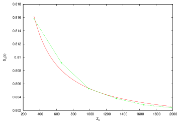
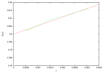
Figure 7: Left panel: Fit of the numerical data for $S_{x}$ corresponding to $N=7\cdot 10^{6}$, with $f(x)=a_{0}+\frac{a_{1}}{Z_{x}}$, $a_{0}=0.7998$ and $a_{1}=5.3847$. Right panel: Same curve as in the left panel, plotted vs. the variable $\epsilon=1/Z_{x}$, to extrapolate the asymptotic value $S_{x}\simeq 0.8$.

Figures 8 and 9 further prove that $S_{\alpha}$ is always a finite quantity in the Henon case while, in the baker case, it diverges logarithmically only when $S_{\alpha}$ tends to $\pi/2$, which is the only angle for which the projected invariant measure is singular. Therefore, the response can be obtained from the invariant measure at all perturbation angles in the case of the Henon map, and at all but a single angle for the Baker map.

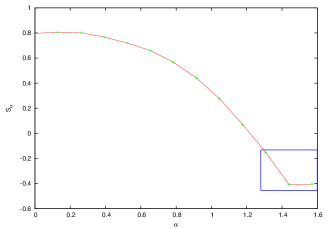
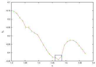
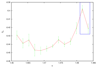
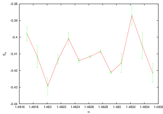
Figure 8: Numerical data with error bars, for the Shannon Entropy $S_{\alpha}$ of the Henon map (13), as a function of the angle $\alpha\in[0,\pi/2]$ with respect to the horizontal direction, at increasing orders of magnification. The top right panel is a magnification of the framed part of the top left panel. The bottom left panel is a magnification of the framed part of the top right panel. The bottom right panel is a magnification of the framed part of the bottom left panel. The quantity $S_{\alpha}$ is quite structured, especially for $\alpha$ close to $\pi/2$, but it is a finite quantity.

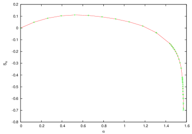
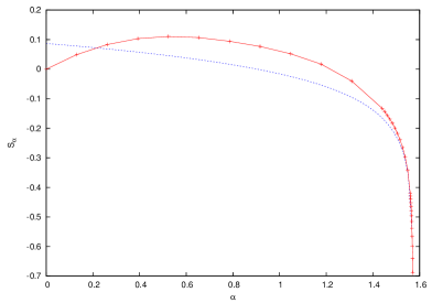
Figure 9: Left panel: Numerical data, supplemented by error bars, for the Shannon Entropy $S_{\alpha}$ of the Baker map (11), as a function of the angle $\alpha\in[0,\pi/2]$ with respect to the $x$-axis. Right panel: Fit of $S_{\alpha}$ for the Baker map, with the curve $f(\alpha)=a\log(\frac{\pi}{2}-\alpha)+b$, $a=-0.101524\pm 0.002768$, and $b=0.0411212\pm 0.01401$. In this case, $S_{\alpha}$ is a much simpler function of $\alpha$ than in the Henon case, and it diverges in the $\alpha\to\pi/2$ limit, because the projected invariant measure is singular at $\alpha=\pi/2$.

This confirms the applicability of a generalized FDT, which yields the response function in terms of the unperturbed state only, even if supported on a fractal set, except in very special situations, such as a negligible set in cases in which the invariant measure is the product of regular and singular mesaures. In particular, for the baker map, the response to a perturbation may be expressed just in terms of the smooth projected invariant measure if one does not perturb uniquely the vertical coordinates. For the Henon map, all directions lead to the existence of a projected invariant measure, although very finely structured.

4 Conclusions

In this paper we have reviewed the methods proposed by Ref. [10] and by Refs. [6, 14], concerning the derivation of response formulae for systems in nonequilibrium steady states. In particular, we have shown that the idea of [14], which is based on the existence of a smooth invariant probability density, may be applied quite generally, with suitable adjustments, to dissipative deterministic dynamics. This requires that projected distributions be considered, rather than the full phase space distributions, becuase projected distributions are usually regular. Only very special combinations of dynamics and perturbations seem to prevent this approach, although in low dimensional dynamics such as ours, the projected distribution functions appear to be quite complex and not smooth.

The presence of noise, in any physically relevant dynamical system, does contribute to smooth out the invariant density, but even in the absence of noise, the fact that statistical mechanics is typically interested in projected dynamics allows an approach to FDT which only requires the properties of the unperturbed states, as in standard response theory. Clearly, this is better and better justified as the dimensionality of the phase space grows. In particular, it is appropriate for macroscopic systems in nonequilibrium steady states, because the dynamics of interest take place in a space whose dimensionality is enormously smaller than that of the phase space. Then, as projecting out more and more produces smoother and smoother distributions, one finds that the approach of Ref.[14] can be used to obtain the linear response function about nonequilirium steady states, from the unperturbed measure only.

Our results support the idea that the projection procedure makes unnecessary the explicit calculation of the term discovered by Ruelle, which was supposed to forbid the standard approach. This does not mean that Ruelle’s term is necessarily negligible [13]. However, except in very peculiar situations, such as our maker map which has carefully oriented manifolds, and for carefully chosen perturbations, that term does not need to be explicitly computed and the calculation of response may be carried out referring only to the unperturbed dynamics, as in the standard cases.

References

References

-
[1]
L. Onsager,
Reciprocal relations in irreversible processes I. Phys. Rev. 37, 405 (1931); Reciprocal relations in irreversible processes II. Phys. Rev. 38, 2265 (1931) -
[2]
M.S. Green,
Markoff random processes and the statistical mechanics of time-dependent phenomena,
J. Chem. Phys. 20 1281 (1952). -
[3]
M.S. Green,
Markoff random processes and the statistical mechanics of time-dependent phenomena: II. Irreversible processes in fluids,
J. Chem. Phys. 22 398 (1954). -
[4]
R. Kubo,
Statistical-mechanical theory of irreversible processes: I. General theory and simple applications to magnetic and conduction problems J. Phys. Soc. Japan 12 570 (1957). - [5] M. Cencini, F. Cecconi, and A. Vulpiani: Chaos: From Simple Models to Complex Systems, (World Scientific, Singapore, 2009).
- [6] U. Marini Bettolo Marconi, A. Puglisi, L. Rondoni, A. Vulpiani: Fluctuation-Dissipation: Response Theory in Statistical Physics, Phys. Rep. 461, 111 (2008).
-
[7]
M. Colangeli, C. Maes, B. Wynants,
A meaningful expansion around detailed balance,
J. Phys. A: Math. Theor. 44 095001 (2011). -
[8]
R. Zwanzig,
Nonequilibrium Statistical Mechanics,
Oxford University Press (2001). -
[9]
M. Colangeli, M. Kröger, H.C. Öttinger,
Boltzmann Equation and hydrodynamic fluctuations, Phys. Rev. E 80, 051202 (2009). -
[10]
D. Ruelle,
General linear response formula in statistical mechanics, and the fluctuation-dissipation theorem far from equilibrium Physics Letters A 245, 220 (1998). -
[11]
D. Evans, L. Rondoni,
Comments on the Entropy of Nonequilibrium Steady States,
J. Stat. Phys. 109, 3/4 (2002). -
[12]
F. Bonetto, A. Kupiainen, J.L. Lebowitz,
Absolute continuity of projected SRB measures of coupled Arnold cat map lattices,
Ergod. Th. & Dynam. Sys. 25, 59 (2005). -
[13]
B. Cessac, J.-A. Sepulchre,
Linear response, susceptibility and resonances in chaotic toy models Physica D 225, 13 (2007). -
[14]
G. Boffetta, G. Lacorata,S. Musacchio, A. Vulpiani,
Relaxation of finite perturbations: beyond the fluctuation dissipation relation,
Chaos, 13, 3 (2003).