The Reactive Energy of Transient EM Fields

I The reactive energy density ${\mathcal{R}}({\boldsymbol{r}},t)$

We give a physically compelling definition of the instantaneous reactive energy density associated with an arbitrary time-domain electromagnetic field in vacuum [2]. In Heaviside-Lorentz units, where $\varepsilon_{0}=\mu_{0}=1$, it is given in terms of the energy density $U({\boldsymbol{r}},t)$ and the Poynting vector ${\boldsymbol{S}}({\boldsymbol{r}},t)$ by

$${\mathcal{R}}({\boldsymbol{r}},t)=\sqrt{U({\boldsymbol{r}},t)^{2}-{\boldsymbol{S}}({\boldsymbol{r}},t)^{2}}.$$ (1)

This is a field-theoretic version of the rest energy of a relativistic point particle with total energy $E$ and momentum ${\boldsymbol{p}}$,

$$E_{0}=\sqrt{E^{2}-c^{2}{\boldsymbol{p}}^{2}}.$$

We may interpret (1) as follows: at space-time points $({\boldsymbol{r}},t)$ where $|{\boldsymbol{S}}|<U$, the energy flow is insufficient to carry away all of the energy in the form of radiation. The (momentarily) abandoned ‘rest’ energy is reactive.

In terms of the electric and magnetic fields $({\boldsymbol{E}},{\boldsymbol{B}})$, we have

$$U=\tfrac{1}{2}({\boldsymbol{E}}^{2}+{\boldsymbol{B}}^{2}),\qquad{\boldsymbol{S}}={\boldsymbol{E}}\times{\boldsymbol{B}}$$

and ${\mathcal{R}}$ reduces to the simple expression

$${\mathcal{R}}=\sqrt{\tfrac{1}{4}({\boldsymbol{E}}^{2}-{\boldsymbol{B}}^{2})^{2}+({\boldsymbol{E}}\cdot{\boldsymbol{B}})^{2}}\geq 0.$$ (2)

This shows that at each space-time point $({\boldsymbol{r}},t)$ we have

$${\mathcal{R}}=0\ \Leftrightarrow\ {\boldsymbol{E}}^{2}-{\boldsymbol{B}}^{2}=0\ \ \hbox{and}\ \ {\boldsymbol{E}}\cdot{\boldsymbol{B}}=0,$$ (3)

which are precisely the conditions for a pure radiation field. For a generic EM field, ${\mathcal{R}}$ is strictly positive almost everywhere in space-time and approaches zero, as it must, only in the far zone. Fields for which ${\mathcal{R}}$ vanishes identically, called null fields, consist of pure radiation. The simplest null fields are traveling plane waves. An interesting example of null fields with sources, resembling a spinning black hole in general relativity, was constructed in [3]. It was this example that inspired the general study of reactive energy density in [2].

Just as the rest energy $E_{0}$ defines the mass $m$ of the point particle by $E_{0}=mc^{2}$, so does ${\mathcal{R}}$ define the electromagnetic inertia density ${\mathcal{I}}$ by

$${\mathcal{R}}({\boldsymbol{r}},t)={\mathcal{I}}({\boldsymbol{r}},t)c^{2}.$$

Whereas $m$ and $E_{0}$ measure impedance to acceleration, ${\mathcal{I}}$ and ${\mathcal{R}}$ measure impedance to radiation. Like $E_{0}$, ${\mathcal{R}}$ is Lorentz invariant, i.e., it has identical values in all uniformly moving (inertial) coordinate frames. For narrowband fields, the time average of ${\mathcal{R}}$ is expected to reduce to the known, stationary reactive energy density. Thus ${\mathcal{R}}$ is a transient or ‘ultra-wideband’ version of the latter, local in time as well as space.

We compute ${\mathcal{R}}({\boldsymbol{r}},t)$ explicitly for two fields representing the extremes of space-time localization:

1. A general time-dependent electric dipole field. This is local in space-time.

2. A standing plane wave obtained by adding two plane waves of frequency $\omega>0$ traveling along $\pm{\boldsymbol{\hat{z}}}$. This is localized at two points in the 4D frequency-wavenumber domain, hence highly nonlocal in space-time.

In Example 1, we find that the reactive energy oscillates around the dipole, as shown in Figure 1, and decays to zero in the far zone as expected.

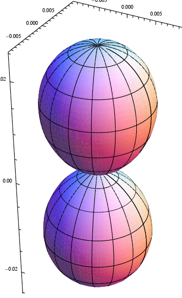
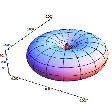
Figure 1: For a frequency-modulated Gaussian electric dipole, the near-field pattern of the reactive energy density oscillates between the two forms shown above; see [2] for details.

In Example 2, we have

$$\begin{aligned} U&=E^{2}[\cos^{2}(kz-\omega t)+\cos^{2}(kz+\omega t)]\\ {\boldsymbol{S}}&={\boldsymbol{\hat{z}}}E^{2}[\cos^{2}(kz-\omega t)-\cos^{2}(kz+\omega t)],\end{aligned}$$ (4)

where $k=\omega/c$ and $E$ is the amplitude of the electric fields of the traveling plane waves. This gives

$${\mathcal{R}}=2E^{2}|\cos(kz-\omega t)\cos(kz+\omega t)|.$$ (5)

Thus ${\mathcal{R}}$ vanishes on the traveling nodal planes $z=z_{\ell}^{\,\scriptscriptstyle\pm}{(t)}$, where

$$z_{\ell}^{\,\scriptscriptstyle\pm}{(t)}=\frac{(2\ell+1)\pi}{2k}\pm ct,\quad\ell=0,\pm 1,\pm 2,\cdots,$$ (6)

and ${\mathcal{R}}>0$ elsewhere. This is shown in Figure 2.

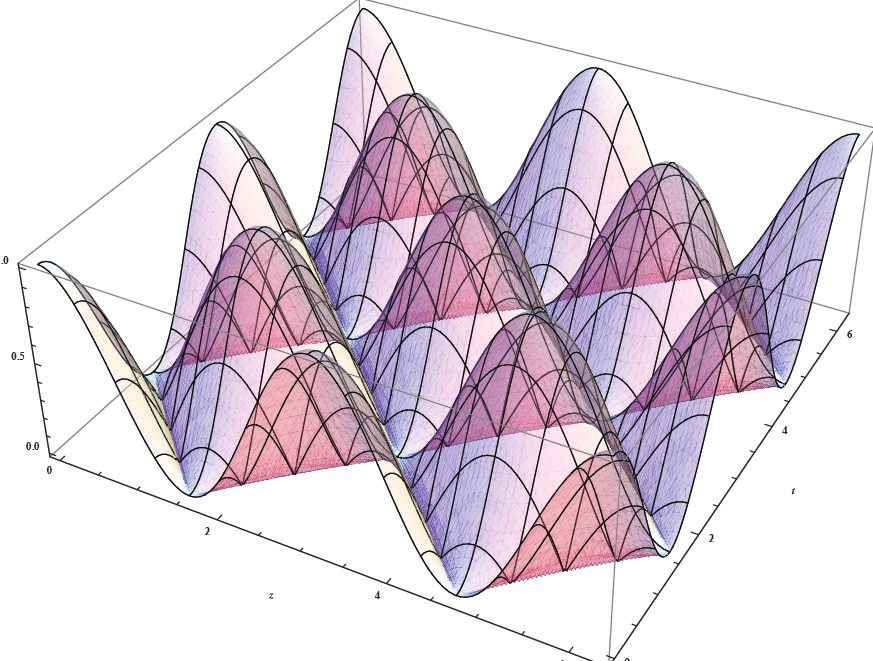
Figure 2: The reactive energy density ${\mathcal{R}}(z,t)$ of the standing plane wave in Example 2, showing the moving nodes (6) where ${\mathcal{R}}=0.$

The two plane waves traveling along $\pm{\boldsymbol{\hat{z}}}$ are null, i.e., their reactive energy densities vanish. Hence the reactive energy of their sum, the standing wave, is due entirely to the interference between the two traveling waves. That is, the invariants in (3) consist only of the cross-terms. Furthermore, since every globally sourceless field is a Fourier superposition of null plane waves with $\omega=ck$, it follows that the reactive energy of every globally sourceless EM field is due entirely to self-interference. This gives a partial intuitve explanation of EM rest energy, as seen most clearly in the standing wave example. However, the rest energy of fields with sources need not be entirely due to self-interference since their Fourier synthesis also requires plane waves with $\omega\neq ck$, which are not null. (Such plane waves represent ‘virtual photons,’ which have positive mass.)

II The energy flow velocity ${\boldsymbol{v}}({\boldsymbol{r}},t)$

The correspondence between the rest energy $E_{0}$ of a relativistic point particle and the reactive energy density ${\mathcal{R}}({\boldsymbol{r}},t)$ of an EM field in vacuum can be extended to include the velocity of the point particle,

$${\boldsymbol{v}}=\frac{c^{2}{\boldsymbol{p}}}{E},$$ (7)

whose field-theoretic version is

$${\boldsymbol{v}}({\boldsymbol{r}},t)=\frac{c{\boldsymbol{S}}({\boldsymbol{r}},t)}{U({\boldsymbol{r}},t)}.$$ (8)

Poynting’s theorem $\partial_{t}U+c\nabla\cdot{\boldsymbol{S}}=-{\boldsymbol{J}}\cdot{\boldsymbol{E}}$ then becomes

$$\partial_{t}U+\nabla\cdot({\boldsymbol{v}}U)=-{\boldsymbol{J}}\cdot{\boldsymbol{E}},$$ (9)

which shows that $U$ behaves like the density of a compressible fluid with source $-{\boldsymbol{J}}\cdot{\boldsymbol{E}}$, flowing at velocity ${\boldsymbol{v}}({\boldsymbol{r}},t)$. Note that

$$v({\boldsymbol{r}},t)\equiv|{\boldsymbol{v}}({\boldsymbol{r}},t)|=c\ \Leftrightarrow\ {\mathcal{R}}({\boldsymbol{r}},t)=0.$$ (10)

Thus, while the field $({\boldsymbol{E}},{\boldsymbol{B}})$ propagates at $c$, its energy generally flows at $v<c$ almost everywhere.

For the standing plane wave of Example 2, (4) shows that $|{\boldsymbol{v}}|\leq c$ as expected, and

$${\boldsymbol{v}}={\boldsymbol{0}} \ \Leftrightarrow\ \cos^{2}(kz-\omega t)=\cos^{2}(kz+\omega t)$$

$$\ \Leftrightarrow\ kz+\omega t=\pm(kz-\omega t)+n\pi.$$

Hence ${\boldsymbol{v}}$ has fixed nodes in both space and time:

$${\boldsymbol{v}}={\boldsymbol{0}}\ \Leftrightarrow\ z=\frac{n\pi}{2k}\equiv z_{n}\ \ \hbox{or}\ \ \ t=\frac{n\pi}{2\omega}\equiv t_{n}$$ (11)

where $n$ is any integer. Since ${\boldsymbol{v}}$ changes sign at $z_{n}$ and $t_{n}$, the energy is totally reflected at these nodes.

The energy oscillates back and forth between the nodal planes $z=z_{n}$, and $v(z,t)\equiv{\boldsymbol{\hat{z}}}\cdot{\boldsymbol{v}}$ oscillates between $\pm c$ at any $z$.

The conflict between the moving nodes (6), where $v=\pm c$, and the stationary nodes (11), where $v=0$, is resolved by noting that $v(z,t)$ is undefined when $U=0$ and ${\boldsymbol{S}}={\boldsymbol{0}}$, so

$$\cos(kz-\omega t)=\cos(kz+\omega t)=0.$$

This gives $\cos kz\cos\omega t=0$ and $\sin kz\sin\omega t=0$, hence

$$z=z_{n}\ \hbox{and}\ t=t_{m}\ \hbox{with $m+n$ odd}.$$

These planes are the intersections of the traveling and stationary nodes. Intuitively, the reason why $v(z,t)$ is undefined at these events is that perfect reflection there requires it to change instantaneously between the values $\pm c$. At all other values of $z$, $v(z,t)$ still oscillates between $\pm c$ but does so in a continuous manner; see Figure 6 in [2].

III A historical note

The fact that the energy of an EM field in vacuum generally flows at speeds less than $c$ was noted almost a century ago by Bateman [4, page 6]. To the best of my knowledge, this important insight has remained undeveloped and largely unappreciated. I believe this phenomenon, and its relation to reactive energy as detailed in [2], are fundamental features of electromagnetic fields which ought to be studied both theoretically and experimentally.

References

- [1]
- [2] G Kaiser, Electromagnetic inertia, reactive energy, and energy flow velocity. J. Phys. A: Math. Theor. 44 (2011) 345206.
- [3] G Kaiser, Coherent electromagnetic wavelets and their twisting null congruences. Preprint, 2011. http://arxiv.org/abs/1102.0238
- [4] H Bateman, The Mathematical Analysis of Electrical and Optical Wave-Motion, Cambridge University Press, 1915; Dover, 1955