How well-proportioned are lens and prism spaces?

Abstract

The CMB anisotropies in spherical 3-spaces with a non-trivial topology are analysed with a focus on lens and prism shaped fundamental cells. The conjecture is tested that well proportioned spaces lead to a suppression of large-scale anisotropies according to the observed cosmic microwave background (CMB). The focus is put on lens spaces $L(p,q)$ which are supposed to be oddly proportioned. However, there are inhomogeneous lens spaces whose shape of the Voronoi domain depends on the position of the observer within the manifold. Such manifolds possess no fixed measure of well-proportioned and allow a predestined test of the well-proportioned conjecture. Topologies having the same Voronoi domain are shown to possess distinct CMB statistics which thus provide a counter-example to the well-proportioned conjecture. The CMB properties are analysed in terms of cyclic subgroups $Z_{p}$, and new point of view for the superior behaviour of the Poincaré dodecahedron is found.

1 Introduction.

This paper studies the cosmic microwave background (CMB) anisotropies of spherical 3-spaces which tile the 3-sphere ${\cal S}^{3}$. A deck group $\Gamma$ of order $|\Gamma|$ tessellates the 3-sphere ${\cal S}^{3}$ in $|\Gamma|$ domains that are identified. In this way multi-connected manifolds are constructed which provide models for the spatial structure of our Universe. The CMB anisotropies on large angular scales differ from that of the simply-connected ${\cal S}^{3}$ and can serve as a signature for topology. The main motivation for cosmic topology is the low power of the CMB anisotropies that is observed [1, 2] at large angular scales on the microwave sky. This feature can naturally be explained by suitably chosen multi-connected manifolds.

An introduction to the cosmic topology can be found in [3, 4, 5, 6, 7]. An extended discussion of spherical multi-connected manifolds is provided by [8]. Spherical spaces attracted attention by the paper [9] which claims that the low power in CMB anisotropies on large scales can be described by the Poincaré dodecahedral topology. In the sequel this result was investigated and extended to other spherical topologies such as the binary octahedral space and the binary tetrahedral space with respect to their statistical CMB properties, see e. g. [10, 11, 12, 13, 14, 15, 16, 17, 18]. The latter are also termed truncated cube and octahedron. Another class of spherical spaces is provided by the lens spaces $L(p,q)={\cal S}^{3}/Z_{p}$ specified by a cyclic group $Z_{p}$ that are studied in [19]. The fundamental domains of the lens spaces can be visualised by a lens-shaped solid where the two lens surfaces are identified by a $2\pi q/p$ rotation for integers $p$ and $q$ that do not possess a common divisor greater 1 and obey $0<q<p$. For more restriction on $p$ and $q$, see below and [8].

In this paper we analyse the so-called “well-proportioned” conjecture [20] which states that manifolds that stretch in all directions by roughly the same amount yield a stronger suppression of the CMB anisotropies on large angular scales than oddly shaped manifolds. This is a purely geometric criterion that only uses the shape of the fundamental domain, but it ignores how the faces of the fundamental domain are identified. A genuine test of this hypothesis would be provided by two deck groups $\Gamma_{1}$ and $\Gamma_{2}$ that possess fundamental domains with the same geometric shape but with distinct identifications of their faces. Fortunately, such examples exist among spherical multi-connected manifolds.

We put the focus on the lens spaces $L(p,q)$ with $p=4n$ and $q=p/2-1=2n-1$ for the integers $n=2,3,4,\dots$. These lens spaces are inhomogeneous in the sense that the geometric shape of their fundamental domain, defined as a Voronoi domain, and their statistical properties of the CMB anisotropies vary with the position of the CMB observer. This allows a test of the well-proportioned conjecture only in dependence of the position of the CMB observer since all cosmological parameters are held fixed. More important is, however, the fact that the lens spaces $L(p,p/2-1)$ possess for two special observer positions a Voronoi domain identical to those of two homogeneous spherical manifolds. The first case is the homogeneous lens space $L(p,1)$ and second one is the prism space ${\cal D}_{p}={\cal S}^{3}/D^{\star}_{p}$ generated by the binary dihedral group $D^{\star}_{p}$. The prism space ${\cal D}_{p}$ is also termed binary dihedral space. For these two observer positions in $L(p,p/2-1)$ one has thus a genuine test for the well-proportioned conjecture. One can test how far the geometry of the Voronoi domain is reflected in the CMB anisotropies.

The paper [20] that put forward well-proportioned conjecture does not provide a quantitative measure for the property of well-proportioned. Instead, their verbal definition states that “a well-proportioned space being one whose three dimensions are of similar magnitudes.” It is the aim of this paper to put this conjecture on a firmer footing by proposing a quantitative measure for the well-proportioned property. For a number of lens spaces $L(p,q)$ and prism spaces ${\cal D}_{p}$, the CMB anisotropies are analysed with respect to this shape measure. For comparison, we also study the Poincaré dodecahedral topology.

In the first step, one has to give a definition of the fundamental domain ${\cal F}$ with respect to the deck group $\Gamma$ of the multi-connected space. A fundamental domain ${\cal F}$ is defined as a domain which contains every physical point only once. Thus, there is no pair of distinct points $x,x^{\prime}\in{\cal F}$ that can be mapped by elements $g\in\Gamma$ onto each other. The natural definition of a fundamental domain is that of the Voronoi domain which is used in this paper. For cosmological applications it is usual as well as natural to place the CMB observer in the centre of the coordinate system. This facilitates the computation of the CMB anisotropies by exploiting the spherical symmetry of the problem.

Therefore, given a realisation of a deck group $\Gamma$ in the chosen coordinates, it is natural to define the fundamental cell ${\cal F}$ in such a way that the fundamental cell ${\cal F}$ does not contain points which can be transformed by a element $g\in\Gamma$ any closer to the observer sitting in the centre $x_{o}$, i. e.

$$x\in{\cal F}\hskip 5.0pt\hbox{ if }\hskip 5.0ptd(x_{o},x)\;\leq\;d(x_{o},g(x))\hskip 10.0pt\hbox{ for all }g\in\Gamma\hskip 10.0pt,$$ (1)

where $d(x_{1},x_{2})$ measures the spherical distances between the points $x_{1},x_{2}\in{\cal S}^{3}$. A fundamental domain ${\cal F}$ constructed in this natural way is called Voronoi domain.

Let us now turn to the question whether a manifold is homogeneous or inhomogeneous. Consider two observers such that the first observer position can be mapped by a transformation $M\notin\Gamma$ onto the second one. Assume that the first observer determines his Voronoi domain by the group elements $g\in\Gamma$, then the second observer gets his Voronoi domain by a similarity transformation of the group $M^{-1}gM$. If $M$ and $g$ commute for all $g\in\Gamma$, then both observers construct the same Voronoi domain, i. e. the manifold is homogeneous. On the other hand, if $M$ and $g$ do not commute, the constructed Voronoi domain depends on the position of the observer. In this case the manifold is called inhomogeneous.

In [19] the inhomogeneous lens spaces $L(p,q)$ with $q>1$ are investigated only for one special observer which is located at the centre of the spherical lens. For this observer position, none of these lens spaces show small correlations of the CMB on large scales as seen in the data of COBE [1] and WMAP [21]. This leads to the question whether the exploitation of the inhomogeneity of lens spaces leads to viable models. This paper extends our previous work [22] which analyses the CMB anisotropy of the lens space $L(8,3)$ in comparison to that of the lens space $L(8,1)$ and the prism space ${\cal D}_{8}$. In this paper the lens spaces $L(p,1)$ and $L(p,p/2-1)$ as well as the prism spaces ${\cal D}_{p}$ are compared with respect to the well-proportioned conjecture. This comparison is very interesting because it shows how strong the influence of the geometry of the Voronoi domain on the CMB anisotropies is. The CMB anisotropies are also analysed in terms of the cyclic subgroups of Clifford translations of the deck groups, of the transformation behaviour of the deck group on the sphere $S_{\hbox{\scriptsize sls}}$ of last scattering, and of the general observer position.

2 Specification of the spherical manifolds $L(p,q)$ and ${\cal D}_{p}$

In order to specify spherical manifolds, one has to define the representation of the 3-sphere ${\cal S}^{3}$. The 3-space ${\cal S}^{3}$ is embedded in the four-dimensional Euclidean space described by the coordinates

$$\vec{x}\;=\;(x_{0},x_{1},x_{2},x_{3})^{T}\in{\cal S}^{3}\hskip 10.0pt\hbox{ with the constraint }\hskip 10.0pt|\vec{x}\,|=1\hskip 10.0pt,$$

i. e. the 3-space ${\cal S}^{3}$ is considered as the manifold with $x_{0}^{2}+x_{1}^{2}+x_{2}^{2}+x_{3}^{2}=1$. The literature offers several possibilities to choose intrinsic coordinates which in turn determine the representation of the deck group. The real representation operates with $\hbox{SO}(4,\mathbb{R})$ matrices which describe transformations as four-dimensional rotations in the four-dimensional Euclidean space. In this paper, we choose complex coordinates $z_{1}:=x_{0}+\hbox{i}x_{3}$ and $z_{2}:=x_{1}+\hbox{i}x_{2}$ which are used to define the coordinate matrix

$$u\;=\;\left(\begin{array}[]{cc}z_{1}&\hbox{i}z_{2}\\ \hbox{i}\overline{z}_{2}&\overline{z}_{1}\end{array}\right)\;=\;\left(\begin{array}[]{cc}x_{0}+\hbox{i}x_{3}&-x_{2}+\hbox{i}x_{1}\\ x_{2}+\hbox{i}x_{1}&x_{0}-\hbox{i}x_{3}\end{array}\right)\in\hbox{SU}(2,\mathbb{C})\equiv{\cal S}^{3}\hskip 10.0pt.$$ (2)

The intrinsic coordinates $(\rho,\alpha,\epsilon)$ are related to $\vec{x}$ by

$$\left(\begin{array}[]{c}x_{0}\\ x_{1}\\ x_{2}\\ x_{3}\end{array}\right)\;=\;\left(\begin{array}[]{c}\cos\rho\;\cos\alpha\\ \sin\rho\;\cos\epsilon\\ \sin\rho\;\sin\epsilon\\ \cos\rho\;\sin\alpha\end{array}\right)\hskip 10.0pt,\hskip 10.0pt0\leq\rho\leq\frac{\pi}{2}\;\;,\;\;0\leq\alpha,\epsilon\leq 2\pi\hskip 10.0pt,$$ (3)

that is $z_{1}=\cos\rho\,e^{\hbox{\scriptsize i}\alpha}$ and $z_{2}=\sin\rho\,e^{\hbox{\scriptsize i}\epsilon}$. Form these coordinates, one obtains the spherical distance of the point $(\rho,\alpha,\epsilon)$ from the origin

$$\tau(\hat{n})\;=\;\arcsin r(\hat{n})\hskip 10.0pt\hbox{ with }\hskip 10.0ptr(\hat{n})\;=\;\sqrt{x_{1}^{2}+x_{2}^{2}+x_{3}^{2}}\hskip 10.0pt.$$ (4)

In the complex representation, the transformations are determined by two $\hbox{SU}(2,\mathbb{C})$ matrices denoted as the pair $(g_{a},g_{b})$ that acts on the points $u\in\hbox{SU}(2,\mathbb{C})$ of the 3-sphere ${\cal S}^{3}\equiv\hbox{SU}(2,\mathbb{C})$ by left and right multiplication

$$(g_{a},g_{b}):\,u\rightarrow g_{a}^{-1}\,u\,g_{b}\hskip 10.0pt.$$ (5)

For the group of transformations $g=(g_{a},g_{b})$ there is the isomorphism $\hbox{SO}(4,\mathbb{R})\equiv(\hbox{SU}_{a}(2,\mathbb{C})\otimes\hbox{SU}_{b}(2,\mathbb{C}))/\{\pm({\bf 1},{\bf 1})\}$. The identity ${\bf 1}$ is the $2\times 2$ unit matrix in this representation. Compared to the real representation, the complex representation has the advantage of revealing the inhomogeneity of the manifold immediately.

After having defined the transformations $g=(g_{a},g_{b})$ on ${\cal S}^{3}\equiv\hbox{SU}(2,\mathbb{C})$, we can turn to the specification of the spherical lens spaces $L(p,q)$, where $p$ and $q$ have to be relatively prime with $1\leq q<p$. The deck group $\Gamma$ is generated by $g_{L(p,q)}=(g_{a},g_{b})$ with

$$g_{a}\;=\;\hbox{diag}(e^{-\hbox{\scriptsize i}\Psi_{a}},e^{\hbox{\scriptsize i}\Psi_{a}})\hskip 10.0pt\hbox{ and }\hskip 10.0ptg_{b}\;=\;\hbox{diag}(e^{-\hbox{\scriptsize i}\Psi_{b}},e^{\hbox{\scriptsize i}\Psi_{b}})$$ (6)

with $\Psi_{a}=\left(\frac{q+1}{p}\right)\pi$ and $\Psi_{b}=\left(\frac{q-1}{p}\right)\pi$. The complete set of group elements $g_{n}\in\Gamma$ is then obtained by

$$g_{n}\;=\;\Big{(}(g_{a})^{n},(g_{b})^{n}\Big{)}\hskip 10.0pt\hbox{ for }\hskip 10.0ptn=1,\dots,p\hskip 10.0pt.$$ (7)

Two spaces $L(p,q)$ and $L(p^{\prime},q^{\prime})$ are homeomorphic if and only if $p=p^{\prime}$ and either $q=\pm q^{\prime}(\hbox{mod }p)$ or $q\,q^{\prime}=\pm 1(\hbox{mod }p)$ [8]. For example, the lens spaces $L(p,q)$ and $L(p,p-q)$ are mirror images. Then the above restrictions on $p$ and $q$ leave as homogeneous lens spaces only $L(p,1)$ where the generator of the deck group (6) is given by $g_{a}\;=\;\hbox{diag}(e^{-\hbox{\scriptsize i}\frac{2\pi}{p}},e^{\hbox{\scriptsize i}\frac{2\pi}{p}})$ and $g_{b}\;=\;{\bf 1}$ .

Finally we specify the deck group $D^{\star}_{p}$ of the prism space ${\cal D}_{p}$. The two generators $g_{1}=(g_{a1},{\bf 1})$ and $g_{2}=(g_{a2},{\bf 1})$ of the deck group $D^{\star}_{p}$ can be represented by

$$g_{a1}\;=\;\hbox{diag}(e^{-\hbox{\scriptsize i}\Psi_{az}},e^{\hbox{\scriptsize i}\Psi_{az}})\hskip 10.0pt\hbox{ and }\hskip 10.0ptg_{a2}\;=\;\left(\begin{array}[]{cc}\cos(\Psi_{ay})&-\sin(\Psi_{ay})\\ \sin(\Psi_{ay})&\cos(\Psi_{ay})\end{array}\right)$$ (8)

with $\Psi_{az}=2\pi\left(\frac{2}{p}\right)$ and $\Psi_{ay}=2\pi\left(\frac{1}{4}\right)$. The deck group $D^{\star}_{p}$ contains as cyclic subgroups $Z_{p/2}$ and $Z_{4}$ with multiplicity 1 and $p/4$, respectively, for more details see [8].

3 Transformation of the CMB observer

Let us now address the question how the group elements $g\in\Gamma$ transform under a change of the observer position, whereby each observer naturally puts his position at the origin of his coordinate system. The behaviour under such transformations will lead to the distinction between homogeneous and inhomogeneous manifolds. By applying an arbitrary isometry $t$ to the coordinates

$$u\rightarrow u^{\prime}=u\,t\;\;,\;\;t\in\hbox{SU}(2,\mathbb{C})\hskip 10.0pt,$$ (9)

the origin of the coordinate system can be transformed to every point on ${\cal S}^{3}$. Now consider a given point which coordinate matrices with respect to two observers $o$ and $o^{\prime}$ are related by $u^{\prime}=ut$. Assume that the group elements of the observer $o$ are given by $g_{n}=(g_{an},g_{bn})$, $n=1,2,\dots$. Every point $u$ on the 3-sphere is mapped by $g_{n}$ to points $\tilde{u}_{n}$ which are to be identified $\tilde{u}_{n}\equiv(g_{an})^{-1}\,u\,g_{bn}$. The transformation of the points $\tilde{u}_{n}$ into the coordinate system of observer $o^{\prime}$ results in

$$\tilde{u}_{n}\rightarrow\tilde{u}^{\prime}_{n}=\tilde{u}_{n}\,t = (g_{an})^{-1}\,u\,g_{bn}\,t$$ (10)

$$= (g_{an})^{-1}\,u\,t\,(t^{-1}\,g_{bn}\,t)=(g_{an})^{-1}\,u^{\prime}\,(t^{-1}\,g_{bn}\,t)\hskip 10.0pt.$$

The observer $o^{\prime}$ uses the equation $\tilde{u}^{\prime}_{n}=(g^{\prime}_{an})^{-1}\,u^{\prime}\,g^{\prime}_{bn}$ in order to identify points on the 3-sphere. Comparing this equation with eq. (10), one gets the deck transformations

$$g^{\prime}_{n}\;=\;(g^{\prime}_{an},g^{\prime}_{bn})\;=\;(g_{an},t^{-1}\,g_{bn}\,t)\hskip 10.0pt,\hskip 10.0ptn=1,2,\dots\hskip 10.0pt,$$ (11)

with respect to the observer $o^{\prime}$. Since the coordinate transformation $t$ is given as right action, the left action $g_{an}$ of a deck transformation $g_{n}$ does not chance, but the right action $g_{bn}$ of a deck transformation $g_{n}$ chances under a coordinate transformation $t$, in general.

In the case of the manifolds $L(p,1)$ and ${\cal D}_{p}$ the action of the group can be given as a pure left action. This is the reason why their group elements and their Voronoi domains are unchanged under an isometry $t$, and these manifolds are called homogeneous. In contrast the deck groups of the lens spaces $L(p,q)$ with $q>1$ are always given by right and left action. Therefore, the action of the isometry $t$ changes the group elements as well as the Voronoi domains of these inhomogeneous manifolds.

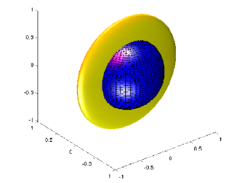
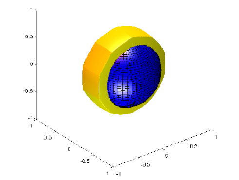
Figure 1: The Voronoi domain for the inhomogeneous $L(20,9)$ space is shown in yellow. In panel (a) the observer position is $\rho=0$ and the Voronoi domain is identical to that of the homogeneous $L(20,1)$ lens space. Choosing for the observer position $\rho=\pi/4$ the prism shaped Voronoi domain shown in panel (b) is obtained which is identical to that of the prism space ${\cal D}_{20}$. In both figures the sphere $S_{\hbox{\scriptsize sls}}$ of last scattering is depicted as a blue sphere having a radius $\tau_{\hbox{\scriptsize sls}}=0.6$. This value corresponds to $\Omega_{\hbox{\scriptsize tot}}=1.04$. Smaller values of $\Omega_{\hbox{\scriptsize tot}}$ lead to even smaller spheres, see figure 4(a).

In the following the position of the observer is shifted using the parameterisation

$$t(\rho,\alpha,\epsilon)\;=\;\left(\begin{array}[]{cc}\cos(\rho)\,e^{+\hbox{\scriptsize i}\alpha}&\hbox{i}\sin(\rho)\,e^{+\hbox{\scriptsize i}\epsilon}\\ \hbox{i}\sin(\rho)\,e^{-\hbox{\scriptsize i}\epsilon}&\cos(\rho)\,e^{-\hbox{\scriptsize i}\alpha}\end{array}\right)$$ (12)

with $\rho\in[0,\frac{\pi}{2}]$, $\alpha,\epsilon\in[0,2\pi]$. The transformation (12) maps the group elements (7) generated by (6) according to (11) onto $g^{\prime}_{n}\;=\;(g^{\prime}_{an},g^{\prime}_{bn})$ with

$$g^{\prime}_{an}=\hbox{diag}(e^{-\hbox{\scriptsize i}\,n\Psi_{a}},e^{\hbox{\scriptsize i}\,n\Psi_{a}})$$ (13)

and

$$g^{\prime}_{bn}=\left(\begin{array}[]{ll}\cos(n\Psi_{b})-\hbox{i}\sin(n\Psi_{b})\cos(2\rho)&\sin(2\rho)e^{\hbox{i}\left(\epsilon-\alpha\right)}\sin(n\Psi_{b})\\ -\sin(2\rho)e^{-\hbox{i}\left(\epsilon-\alpha\right)}\sin(n\Psi_{b})&\cos(n\Psi_{b})+\hbox{i}\sin(n\Psi_{b})\cos(2\rho)\end{array}\right)\hskip 4.0pt.$$ (16)

$\Psi_{a}$ and $\Psi_{b}$ are defined below eq. (6).

The above description of the spherical space also allows a visualisation of the Voronoi domains by projecting $\vec{x}$, see eq. (3), down to the three-dimensional space $(x_{1},x_{2},x_{3})^{T}$, i. e. by simply omitting the $x_{0}$ coordinate. The Voronoi cell is computed with respect to an observer at the origin $\vec{x}_{0}=(1,0,0,0)$ by using the group elements (13) of $L(p,q)$ for $\alpha,\epsilon=0$. For the space $L(20,9)$ two Voronoi domains are visualised in this way in figure 1, where two different observer positions are chosen. To give an impression of the size of the sphere $S_{\hbox{\scriptsize sls}}$ of last scattering, it is depicted for a radius $\tau_{\hbox{\scriptsize sls}}=0.6$ which corresponds to the largest sphere which is compatible with the present cosmological parameters.

4 The eigenmodes of spherical manifolds

4.1 The eigenmodes of the 3-sphere ${\cal S}^{3}$

The eigenmodes of the simply-connected spherical manifold ${\cal S}^{3}$ can be generated by the Lie algebra of $\hbox{SO}(4,\mathbb{R})\equiv(\hbox{SU}_{a}(2,\mathbb{C})\otimes\hbox{SU}_{b}(2,\mathbb{C}))/\{\pm({\bf 1},{\bf 1})\}$. The abstract generators satisfy the relations

$$[J_{ax},J_{ay}]\;=\;\hbox{i}\,J_{az}\hskip 10.0pt,\hskip 10.0pt[J_{bx},J_{by}]\;=\;\hbox{i}\,J_{bz}\hskip 10.0pt\hbox{and cyclic permutations.}$$ (17)

The components of $\vec{J}_{a}=(J_{ax},J_{ay},J_{az})\in\hbox{SU}_{a}(2,\mathbb{C})$ commute with all components of $\vec{J}_{b}=(J_{bx},J_{by},J_{bz})\in\hbox{SU}_{b}(2,\mathbb{C})$. The eigenmodes of $\vec{J}_{a}$ obey

$${\vec{J}_{a}}^{\;2}|j_{a},m_{a}\rangle = j_{a}(j_{a}+1)|j_{a},m_{a}\rangle\hskip 10.0pt,\hskip 10.0ptj_{a}\in\frac{\mathbb{N}_{0}}{2}$$ (18)

$$J_{az}|j_{a},m_{a}\rangle = m_{a}|j_{a},m_{a}\rangle\hskip 10.0pt,\hskip 10.0pt|m_{a}|\leq j_{a}\hskip 10.0pt,$$ (19)

and similarly for $\vec{J}_{b}$. The complete basis in respect of $\hbox{SO}(4,\mathbb{R})$ factorises as

$$|j;m_{a},m_{b}\rangle\;:=\;|j,m_{a}\rangle\,|j,m_{b}\rangle\hskip 10.0pt.$$ (20)

The Laplace-Beltrami operator $\Delta$ on the 3-sphere ${\cal S}^{3}$ can be written as

$$-\Delta\;=\;2\Big{(}{\vec{J}_{a}}^{\;2}+{\vec{J}_{b}}^{\;2}\Big{)}\hskip 10.0pt.$$

Thus, the eigenmodes with the eigenvalue $E_{j}:=4j(j+1)=\beta^{2}-1$ of the operator $-\Delta$ are given by eq. (20) where we defined $\beta:=2j+1$. An equivalent representation of the eigenmodes $|j;m_{a},m_{b}\rangle$ is given by $|j;l,m\rangle$ where $l$ is the eigenvalue of $\vec{L}:=\vec{J}_{a}+\vec{J}_{b}$. These two representations of the eigenmodes are connected by

$$|j;m_{a},m_{b}\rangle = \sum_{l}\langle jm_{a}jm_{b}|lm\rangle\;|j;l,m\rangle$$ (21)

$$|j;l,m\rangle = \sum_{m_{a}}\langle jm_{a}jm_{b}|lm\rangle\;|j;m_{a},m_{b}\rangle\hskip 10.0pt$$

where the $\langle jm_{a}jm_{b}|lm\rangle$ are the Clebsch-Gordan coefficients [23]. In general, $\langle jm_{a}jm_{b}|lm\rangle\neq 0$ only for $0\leq l\leq 2j$ and $m_{a}+m_{b}=m$.

4.2 The eigenmodes of the lens spaces $L(p,q)$

The action of the generator (6) of the lens space $L(p,q)$ on the eigenmodes (20) can be written as $U_{g}=e^{\hbox{\scriptsize i}2\psi_{a}J_{az}}e^{\hbox{\scriptsize i}2\psi_{b}J_{bz}}$ with $\psi_{a}$ and $\psi_{b}$ defined below eq. (6). The eigenmodes on the lens space $L(p,q)$ invariant under the action of $U_{g}$ are

$$|j;m_{a},m_{b}\rangle\hskip 10.0pt\hbox{with}\hskip 10.0pt(q+1)\,m_{a}+(q-1)\,m_{b}\equiv 0\;{\rm mod}\;p\hskip 10.0pt,$$ (22)

where $\left|m_{a}\right|,\left|m_{b}\right|\leq j$. In general, similar eigenmodes on the lens spaces are reported in [24] and equivalent sets of eigenmodes on the lens spaces in [25, 26].

4.3 The eigenmodes of the prism spaces ${\cal D}_{p}$

In the chosen notation the action of the two generators (8) of the prism space ${\cal D}_{p}$ are given by $U_{g_{1}}=e^{\hbox{\scriptsize i}2\psi_{az}J_{az}}$ and $U_{g_{2}}=e^{\hbox{\scriptsize i}2\psi_{ay}J_{ay}}$ with $\psi_{az}$ and $\psi_{ay}$ defined below eq. (8). The eigenmodes on the prism space ${\cal D}_{p}$ invariant under the action of $U_{g_{1}}$ and $U_{g_{2}}$ are

$$\begin{array}[]{ll}\frac{1}{\sqrt{2}}\left(|j;m_{a},m_{b}\rangle+(-1)^{m_{a}}\,|j;-m_{a},m_{b}\rangle\right)&:\;j\;\hbox{even},m_{a}>0\\ |j;m_{a},m_{b}\rangle&:\;j\;\hbox{even},m_{a}=0\\ \frac{1}{\sqrt{2}}\left(|j;m_{a},m_{b}\rangle-(-1)^{m_{a}}\,|j;-m_{a},m_{b}\rangle\right)&:\;j\;\hbox{odd},m_{a}>0\end{array}\hskip 10.0pt,$$ (26)

where $j\in\mathbb{N}_{0}\setminus\{1,3,\dots,2[\frac{p}{8}]-1\}$, $m_{b}\in\mathbb{Z}$, $m_{a}\in\mathbb{N}_{0}$, $m_{a}\equiv 0\;\hbox{mod}\;p/4$, and $m_{a},\left|m_{b}\right|\leq j$. In general, similar eigenmodes on these manifolds are given in [25, 24, 27].

4.4 The observer dependence of the eigenmodes on lens spaces $L(p,q)$

The operator, which corresponds to the transformation to a new observer as discussed in sec. 3, can be given by

$$D(t)\;=\;D(\alpha+\epsilon,2\rho,\alpha-\epsilon)\;=\;e^{\hbox{\scriptsize i}(\alpha+\epsilon)J_{bz}}\,e^{\hbox{\scriptsize i}(2\rho)J_{by}}\,e^{\hbox{\scriptsize i}(\alpha-\epsilon)J_{bz}}\hskip 10.0pt,$$ (27)

where the coordinates (12) are used for the observer. The action of this operator on the eigenmodes results in

$$D(t^{-1})|j;m_{a},m_{b}\rangle\; = \;\sum_{\tilde{m}_{b}=-j}^{j}D^{\,j}_{\tilde{m}_{b},m_{b}}(t^{-1})|j;m_{a},\tilde{m}_{b}\rangle$$

$$\hbox{with}\hskip 10.0pt(q+1)\,m_{a}+(q-1)\,m_{b}\equiv 0\;{\rm mod}\;p$$

where the completeness relation $\sum_{\tilde{m}_{b}=-j}^{j}|j,\tilde{m}_{b}\rangle\langle j,\tilde{m}_{b}|=1$ and the definition of the $D$-function, also called Wigner polynomial,

$$D^{\,j}_{\tilde{m}_{b},m_{b}}(t)\; := \;\langle j,\tilde{m}_{b}|D(t)|j,m_{b}\rangle$$

$$= \;e^{\hbox{i}\,(\alpha+\epsilon)\,\tilde{m}_{b}}d^{\,j}_{\tilde{m}_{b},m_{b}}(2\rho)e^{\hbox{i}\,(\alpha-\epsilon)\,m_{b}}\hskip 10.0pt$$ (29)

are used. The numerical values of the $d$ function are computed by the algorithm described in [28]. With eq. (21) the expansion of the eigenmodes (4.4) on the lens spaces $L(p,q)$ with respect to the spherical basis $|j;l,m\rangle$ yields

$$D(t^{-1})|j;m_{a},m_{b}\rangle = \sum_{l=0}^{2j}\sum_{m=-l}^{l}\xi^{j,i(m_{a},m_{b})}_{lm}(L(p,q);t)\,|j;l,m\rangle\;\;$$

$$\xi^{j,i(m_{a},m_{b})}_{lm}(L(p,q);t) = \langle jm_{a}j\tilde{m}_{b}|lm\rangle\,D^{\,j}_{\tilde{m}_{b},m_{b}}(t^{-1})$$

$$\hbox{with}\hskip 10.0pt(q+1)\,m_{a}+(q-1)\,m_{b}\equiv 0\;{\rm mod}\;p\hskip 10.0pt.$$

Here, the abbreviation $\tilde{m}_{b}:=m-m_{a}$ is introduced, and $1\leq i(m_{a},m_{b})\leq r^{L(p,q)}(\beta)$ counts the multiplicity $r^{L(p,q)}(\beta)$ of the eigenvalue $E_{j}$ of the Laplace-Beltrami operator on $L(p,q)$ for $j\in\frac{\mathbb{N}_{0}}{2}$. The transformation $t$ characterises the position of the observer.

For homogeneous spherical manifolds it is shown in [22] that the same set of eigenmodes can be chosen for all observer position. For example on $L(p,1)$ one can choose the above coefficients to $\xi^{j,i(m_{a},m_{b})}_{lm}(L(p,1))=\langle jm_{a}jm_{b}|lm\rangle$. In contrast for an inhomogeneous lens space $L(p,q)$, $q>1$, such a choice is not possible due to the restriction on $m_{b}$, and one has to use eq. (4.4) which depends on the observer position.

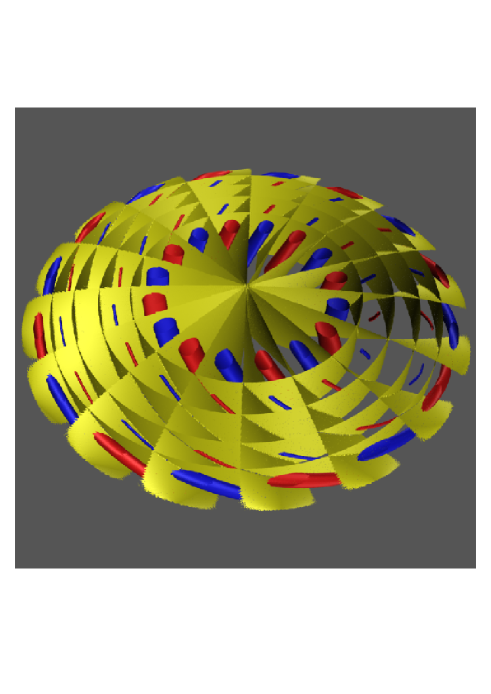
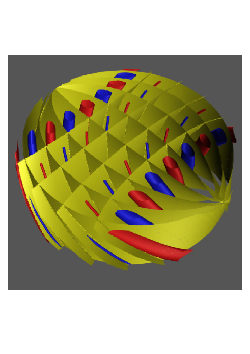
Figure 2: An eigenmode for the inhomogeneous lens space $L(20,9)$ for $\beta=25$ is shown for the lens shaped Voronoi domain $\rho=0$ (left) and for the prism shaped Voronoi domain $\rho=\pi/4$ (right). For intermediate values of $\rho$ the structure of the eigenmode changes continuously between the two cases shown above. The yellow surfaces represents the nodal surface, blue and red corresponds to a negative and a positive equipotential surface.

The eigenmodes $|j;m_{a},m_{b}\rangle$ are only constructed in an abstract way since that is all what is needed. However, it is instructive to compute the eigenmodes as a function of the coordinates $u$ of the spherical space. To that aim, the Wigner basis [29, 22]

$$\psi(j,m_{a},m_{b})(u)\,=\,\frac{2j+1}{\sqrt{2\,\pi^{2}}}\;\langle j-m_{a}jm_{a}|00\rangle\;D^{j}_{-m_{a}m_{b}}(u)\hskip 5.0pt,\;\beta=2j+1\;,$$ (31)

is introduced which is normalised on the 3-sphere ${\cal S}^{3}$. For $\alpha=\epsilon=0$ the eigenmode $\psi^{L(p,q)}_{\rho,\beta,i}(u)$ is obtained by projecting eq. (4.4) onto ${\cal S}^{3}$

$$\psi^{L(p,q)}_{\rho,\beta,i}(u) = \langle u|D(t^{-1})|j;m_{a},m_{b}\rangle$$

$$= \sum_{\tilde{m}_{b}=-j}^{j}D^{\,j}_{\tilde{m}_{b},m_{b}}(t^{-1})\,\langle u|j;m_{a},\tilde{m}_{b}\rangle$$

$$= \sum_{\tilde{m}_{b}=-j}^{j}D^{\,j}_{\tilde{m}_{b},m_{b}}(t^{-1})\,\psi(j,m_{a},\tilde{m}_{b})(u)$$

with the restriction $(q+1)\,m_{a}+(q-1)\,m_{b}\equiv 0\;{\rm mod}\;p$. The dependence on the observer position $\rho$ is determined by the Wigner polynomial $D^{\,j}_{\tilde{m}_{b},m_{b}}(t^{-1})$, eq. (4.4). Thus, one can take an eigenmode $\psi^{L(p,q)}_{\rho,\beta,i}(u)$ and visualise it for various values of $\rho$. For the two interesting positions $\rho=0$ and $\rho=\pi/4$, an eigenmode of $L(20,9)$ for $\beta=25$ is depicted in figure 2.

4.5 The quadratic sum of eigenmodes on spherical spaces

The calculation of the ensemble average of the temperature 2-point correlation function (39) or the multipole spectrum (6.1) on inhomogeneous lens spaces ($q>1$) requires the evaluation of the following quadratic sum:

$$\frac{1}{2l+1}\sum_{m=-l}^{l}\sum_{m_{a},m_{b}}\left|\xi^{j,i(m_{a},m_{b})}_{lm}(L(p,q);t)\right|^{2}$$

$$=\frac{1}{2l+1}\sum_{m=-l}^{l}\sum_{m_{a},m_{b}}\left|\langle jm_{a}j\tilde{m}_{b}|lm\rangle\,D^{\,j}_{\tilde{m}_{b},m_{b}}(t^{-1})\right|^{2}$$

$$=\frac{1}{2l+1}\sum_{m=-l}^{l}\sum_{m_{a},m_{b}}\left|\langle jm_{a}j\tilde{m}_{b}|lm\rangle\,d^{\,j}_{\tilde{m}_{b},m_{b}}(-2\rho)\right|^{2}$$

$$\hbox{with}\hskip 10.0pt(q+1)\,m_{a}+(q-1)\,m_{b}\equiv 0\;{\rm mod}\;p\hskip 10.0pt.$$

In the derivation of eq. (4.5) we have used eq. (4.4) where the coordinates of the observer position on the lens space $L(p,q)$ are parameterised by eq. (12). The above quadratic sum depends only on the coordinate $\rho$, and the analysis of the CMB statistics can be restricted to observer positions with $\alpha=\epsilon=0$ and $\rho\in[0,\frac{\pi}{2}]$. A further reduction of the observer positions to the smaller interval $\rho\in[0,\frac{\pi}{4}]$ is possible on lens spaces $L(p,q)$ which satisfy the condition $p=4n$ and $q=p/2-1=2n-1$ for $n=2,3,4,\dots$. This reduction is shown in [22] for $L(8,3)$ (see eq. (53) in [22]).

manifold ${\cal M}$	wave number spectrum $\{\beta\}$	multiplicity $r^{\cal M}(\beta)$
${\cal S}^{3}$	$\mathbb{N}$	$\beta^{2}$
$L(p,1)$,	$\{1,3,5,\dots,p\}$	$\beta\big{(}2\,\big{[}\frac{\beta-1}{2p}\big{]}+1\big{)}$ for $\beta$ odd
$p$ odd $\geq 1$	$\cup\{n|n\in\mathbb{N},n\geq p+1\}$	$2\beta\big{(}\big{[}\frac{\beta-1}{p}\big{]}-\big{[}\frac{\beta-1}{2p}\big{]}\big{)}$ for $\beta$ even
$L(p,1)$,	$2\mathbb{N}-1$	$\beta\big{(}2\,\big{[}\frac{\beta-1}{p}\big{]}+1\big{)}$
$p$ even $\geq 2$
${\cal D}_{p}$,	$\{1,5,9,\dots,4\left[\frac{p}{8}\right]+1\}$	$\beta\big{(}\big{[}\frac{2(\beta-1)}{p}\big{]}+2\left[\frac{\beta-1}{4}\right]-\frac{\beta-3}{2}\big{)}$
$p/4\geq 2$	$\cup\{2n+1|n\in\mathbb{N},n\geq 2\left[\frac{p}{8}\right]+1\}$
${\cal T}$	$\{1,7,9\}$	$\beta\left(2\left[\frac{\beta-1}{6}\right]+\left[\frac{\beta-1}{4}\right]-\frac{\beta-3}{2}\right)$
	$\cup\{2n+1|n\in\mathbb{N},n\geq 6\}$
${\cal O}$	$\{1,9,13,17,19,21\}$	$\beta\left(\left[\frac{\beta-1}{8}\right]+\left[\frac{\beta-1}{6}\right]+\left[\frac{\beta-1}{4}\right]-\frac{\beta-3}{2}\right)$
	$\cup\{2n+1|n\in\mathbb{N},n\geq 12\}$
	$\{1,13,21,25,31,33,37\}$
${\cal I}$	$\cup\{41,43,45,49,51,53,55,57\}$	$\beta\left(\left[\frac{\beta-1}{10}\right]+\left[\frac{\beta-1}{6}\right]+\left[\frac{\beta-1}{4}\right]-\frac{\beta-3}{2}\right)$
	$\cup\,\{2n+1|n\in\mathbb{N},n\geq 30\}$

Table 1: The spectrum of the eigenvalues $E_{\beta}=\beta^{2}-1$ of the Laplace-Beltrami operator on homogeneous spherical manifolds ${\cal M}$ and their multiplicities $r^{\cal M}(\beta)$ are given. In this table an error in [30, 13, 15] is corrected, and an alternative description of the multiplicity is given for the lens spaces $L(p,1)$ and for the prism spaces ${\cal D}_{p}$. This description leads to a faster numerical handling of the multiplicity. The bracket $[x]$ denotes the integer part of $x$.

In the case of a homogeneous spherical manifold ${\cal M}$ this quadratic sum is independent of the observer position and is given by [11, 12, 13, 31, 15]

$$\frac{1}{2l+1}\sum_{m=-l}^{l}\sum_{m_{a},m_{b}}\left|\xi^{j,i(m_{a},m_{b})}_{lm}({\cal M})\right|^{2}\;=\;\frac{r^{{\cal M}}(\beta)}{\beta^{2}}\hskip 10.0pt,$$ (34)

where $r^{\cal M}(\beta)$ is the multiplicity of the eigenvalue of the Laplace-Beltrami operator on the spherical manifold ${\cal M}$. Since 1995 the multiplicities of the eigenvalues of the Laplace-Beltrami operator on all homogeneous spherical manifolds ${\cal M}$ are known [30], see also table 1. Thus it is not necessary to calculate the expansion coefficients $\xi^{j,i(m_{a},m_{b})}_{lm}({\cal M})$ for homogeneous spherical manifolds. This advantage is exploited in the case of the Poincare dodecahedron ${\cal I}={\cal S}^{3}/I^{\star}$, the binary octahedral space ${\cal O}={\cal S}^{3}/O^{\star}$, and the binary tetrahedral space ${\cal T}={\cal S}^{3}/T^{\star}$. Here $I^{\star}$, $O^{\star}$, and $T^{\star}$ are the binary icosahedral, the binary octahedral, and the binary tetrahedral groups [8, 13]. The binary octahedral space ${\cal O}$ is also called truncated cube. The binary tetrahedral space ${\cal T}$ is also named octahedron because of the geometry of its Voronoi domain [8], however, this notation can be misleading. Eq. (34) is also used for the prism space ${\cal D}_{p}={\cal S}^{3}/D_{p}^{\star}$ and the homogeneous lens space $L(p,1)={\cal S}^{3}/Z_{p}$.

5 Measures of the shape

In order to verify the well-proportioned conjecture quantitatively, one has to define a measure of the shape. Since it is conjectured that shapes with equal dimensions are preferred with respect to a large scale suppression of CMB anisotropies, the shape measure should single out the sphere. For that reason we require that the measure is zero for a sphere, and the larger, the more oddly shaped the Voronoi domain is. With respect to the observer sitting in the centre of the coordinate system, the mean radius $\langle\tau\rangle$ of the Voronoi domain is

$$\langle\tau\rangle\;:=\;\frac{\int d\Omega\,\sin^{2}(\tau(\hat{n}))\;\tau(\hat{n})}{\int d\Omega\,\sin^{2}(\tau(\hat{n}))}\hskip 10.0pt,\hskip 10.0ptd\Omega=\sin\theta\,d\theta\,d\phi\hskip 10.0pt,$$ (35)

where $\tau(\hat{n})$ is the spherical distance to the surface of the Voronoi domain in the direction $\hat{n}$ defined by the angles $\theta$ and $\phi$. The distance $\tau(\hat{n})$ is defined in eq. (4). The variance $\sigma_{\tau}^{2}$ can be taken as a shape measure

$$\sigma_{\tau}^{2}\;:=\;\frac{\int d\Omega\,\sin^{2}(\tau(\hat{n}))\,\Big{(}\langle\tau\rangle-\tau(\hat{n})\Big{)}^{2}}{\int d\Omega\,\sin^{2}(\tau(\hat{n}))}\hskip 10.0pt.$$ (36)

For a hypothetical spherical domain, the variance vanishes. Since the value of the variance $\sigma_{\tau}^{2}$ increases with increasing asymmetry of the Voronoi domain, this variance can serve as a measure of the shape.

The variance (36) can only measure the geometric shape of the Voronoi domain. It ignores, however, the connection of the points on its surface completely. The connection is defined by the deck group which specifies how the faces of the Voronoi domain are mapped onto each other. To every point $\tau(\hat{n})$ of the surface belongs a point $g\tau(\hat{n})$ that also lies on the surface but is obtained from the former by applying one special chosen group element $g\in\Gamma$. The spherical distance between this pair of identified points encodes also the topology and its symmetry. To this end, one defines

$$D\;:=\;\frac{\int d\Omega\;d(\tau(\hat{n}),g\tau(\hat{n}))}{\int d\Omega}\hskip 10.0pt.$$ (37)

We use this quantity with respect to the well-proportioned conjecture but find that models with large CMB anisotropy suppression on large angular scales are not singled out by this measure.

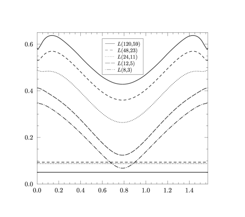
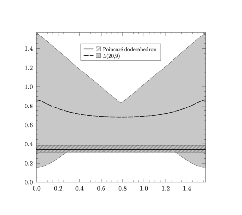
Figure 3: In panel (a) the relative variation $\sigma_{\tau}/\langle\tau\rangle$ of the geometric shape of the Voronoi domain is shown as a shape measure. It is shown for five lens spaces $L(p,p/2-1)$ as a function of the observer position which is parameterised by $\rho$. For $\rho=0$ these lens spaces possess a Voronoi domain of the same geometry as the homogeneous lens spaces $L(p,1)$ and for $\rho=\pi/4$ as the homogeneous prism spaces ${\cal D}_{p}={\cal S}^{3}/D^{\star}_{p}$. For this reason the ratios $\sigma_{\tau}/\langle\tau\rangle$ have the same value for $L(p,p/2-1)$ at $\rho=0$ and $L(p,1)$, and also for $L(p,p/2-1)$ at $\rho=\pi/4$ and ${\cal D}_{p}$. The horizontal lines give the corresponding values of the Poincaré dodecahedron ${\cal I}$ (full line), of the binary octahedral space ${\cal O}$ (dashed line), and of the binary tetrahedral space ${\cal T}$ (dotted line). In panel (b) the mean values $\langle\tau\rangle$ for the lens space $L(20,9)$ and for the Poincaré dodecahedron are diagrammed. In addition the minimal distance $\tau_{\hbox{\scriptsize min}}$ and the maximal distance $\tau_{\hbox{\scriptsize max}}$ from the observer to the surface of the Voronoi domain for these manifolds are represented. The interval between the minimal and the maximal distances is shown as a shaded band for the Poincaré dodecahedron and as a grey area for the lens space $L(20,9)$. Between $\rho$ about 0.275 and 1.296 the lens space $L(20,9)$ has the same minimal distance $\tau_{\hbox{\scriptsize min}}$ as the Poincaré dodecahedron.

In the following we use $\sigma_{\tau}$, i. e. the square root of the variance (36), as a shape measure. Since the manifolds of interest possess Voronoi domains with different volumina, we consider the normalised quantity $\sigma_{\tau}/\langle\tau\rangle$ where $\langle\tau\rangle$ is the mean radius of the Voronoi domain. We investigate this ratio for the lens spaces $L(p,p/2-1)$ in dependence on the observer position which is parameterised by $\rho$. The relative variation $\sigma_{\tau}/\langle\tau\rangle$ is diagrammed in figure 3(a) for the lens spaces belonging to $p=8$, 12, 24, 48, and 120. One observes that the values of $\sigma_{\tau}/\langle\tau\rangle$ increase with the order $p$ of the deck group. For the considered lens spaces $L(p,p/2-1)$ the minimum of $\sigma_{\tau}/\langle\tau\rangle$ is always found at $\rho=\pi/4$. This is a special position of the observer since the lens space $L(p,p/2-1)$ possesses for $\rho=\pi/4$ a Voronoi domain of the same geometrical shape as the prism space ${\cal D}_{p}$. Thus, the lens space $L(p,p/2-1)$ at $\rho=\pi/4$ and the prism space ${\cal D}_{p}$ have the same value for the introduced measure of shape. In addition all lens spaces $L(p,q)$, $q>1$, have the same shape of the Voronoi domain at $\rho=0$ as the homogeneous lens space $L(p,1)$, namely a spherical lens. Therefore, they have also the same value for the ratio $\sigma_{\tau}/\langle\tau\rangle$ which does not contain information about the identification of points on the surface of the lens.

The Poincaré dodecahedron ${\cal I}$, the binary octahedral space ${\cal O}$, and the binary tetrahedral space ${\cal T}$ can describe very good the CMB anisotropies at large scales [12, 13]. For this reason we use the shape measure of these manifolds as reference values. Since these three manifolds are homogeneous, their values of $\sigma_{\tau}/\langle\tau\rangle$ have no $\rho$ dependence and are represented by the horizontal lines in figure 3(a). The figure reveals that only $L(8,3)$ around $\rho=\pi/4$ has values for the shape measure of the same magnitude as the binary polyhedral spaces ${\cal I}$, ${\cal O}$, and ${\cal T}$. If a small value of the ratio $\sigma_{\tau}/\langle\tau\rangle$ implies a good characterisation of the CMB anisotropies, then the results of figure 3(a) would suggest that a good description of the CMB is given only in the case of the lens space $L(8,3)$ and the prism space ${\cal D}_{8}$. In sec. 6.2 and 6.5 we investigate how far this measure of shape can really reflect the properties of the CMB anisotropies on these manifolds.

To give an impression how the value of $\langle\tau\rangle$ depends on the observer position in the case of the lens spaces $L(p,p/2-1)$, the mean value $\langle\tau\rangle$ for the lens space $L(20,9)$ is shown in figure 3(b) together with the minimal value $\tau_{\hbox{\scriptsize min}}$ and the maximal value $\tau_{\hbox{\scriptsize max}}$. It turns out that the maximal value of $\langle\tau\rangle$ for $L(p,q)$ is obtained for the usual lens shaped domain which corresponds in our description to $\rho=0$. The maximal value of $\langle\tau\rangle$ is then the average of the largest and the smallest values of $\tau(\hat{n})$. With $\tau_{\hbox{\scriptsize max}}=\pi/2$ and $\tau_{\hbox{\scriptsize min}}=\pi/p$ for $\rho=0$, this value is

$$\langle\tau\rangle_{\hbox{\scriptsize max}}\;=\;\frac{1}{2}\,\left(\tau_{\hbox{\scriptsize max}}+\tau_{\hbox{\scriptsize min}}\right)\;=\;\frac{\pi}{2}\,\left(\frac{1}{2}+\frac{1}{p}\right)\hskip 10.0pt.$$ (38)

In addition, the values for $\langle\tau\rangle$, $\tau_{\hbox{\scriptsize min}}$, and $\tau_{\hbox{\scriptsize max}}$ of the Poincaré dodecahedron are diagrammed in figure 3(b). An interesting point is that between $\rho$ about 0.275 and 1.296 the lens space $L(20,9)$ has the same value for $\tau_{\hbox{\scriptsize min}}$ as the Poincaré dodecahedron. Why this is important will become clear in sec. 6.3.

Before we discuss the introduced shape measure with respect to the suppression of the CMB anisotropy on large scales, some remarks on the temperature 2-point correlation $C(\vartheta)$ are in order.

6 The CMB anisotropy on spherical spaces and the well-proportioned conjecture

6.1 Calculation of the CMB temperature correlations on spherical spaces

The temperature correlations of the CMB sky with respect to their separation angle $\vartheta$ are an important diagnostic tool. The correlations at large angles $\vartheta$, where the topological signature is expected, are most clearly revealed by the temperature 2-point correlation function $C(\vartheta)$. It is defined as

$$C(\vartheta)\;:=\;\left<\delta T(\hat{n})\delta T(\hat{n}^{\prime})\right>\hskip 10.0pt\hbox{with}\hskip 10.0pt\hat{n}\cdot\hat{n}^{\prime}=\cos\vartheta\hskip 10.0pt,$$ (39)

where $\delta T(\hat{n})$ is the temperature fluctuation in the direction of the unit vector $\hat{n}$. The 2-point correlation function $C(\vartheta)$ is related to the multipole moments $C_{l}$ by

$$C(\vartheta)\;=\;\sum_{l}\,\frac{2l+1}{4\pi}\,C_{l}\,P_{l}\left(\cos\vartheta\right)\hskip 10.0pt.$$ (40)

The ensemble average of $C_{l}$ can be expressed for a lens space $L(p,q)$ by the quadratic sum of the expansion coefficients $\xi^{\beta,i}_{lm}(L(p,q);t)$ as discussed in sec. 4.5

$$C_{l} := \frac{1}{2l+1}\sum_{m=-l}^{l}\left\langle\left|a_{lm}\right|^{2}\right\rangle$$

$$= \sum_{\beta}\frac{T_{l}^{2}(\beta)\;P(\beta)}{2l+1}\sum_{m=-l}^{l}\sum_{i}\left|\xi^{\beta,i}_{lm}(L(p,q);t)\right|^{2}\hskip 10.0pt,$$

with the initial power spectrum $P(\beta)\sim 1/(E_{\beta}\,\beta^{2-n_{\hbox{\scriptsize s}}})$ where $E_{\beta}=\beta^{2}-1$ are the eigenvalues of the Laplace-Beltrami operator on the considered spherical manifold ${\cal M}$, $\beta=2j+1$. Within the framework of this paper the spectral index $n_{\hbox{\scriptsize s}}$ is chosen to $n_{\hbox{\scriptsize s}}=0.961$. $T_{l}(k)$ is the transfer function containing the full Boltzmann physics, e. g. the ordinary and the integrated Sachs-Wolfe effect, the Doppler contribution, the Silk damping and the reionisation are taken into account. The reionisation model of [32] is applied with the reionisation parameters $\alpha=0.4$ and $\beta=9.85$. Using the expression (4.5) for the expansion coefficients $\xi^{\beta,i}_{lm}(L(p,q);t)$ we get for the ensemble average of $C_{l}$ on $L(p,q)$

$$C_{l}\;=\;\sum_{\beta}\frac{T_{l}^{2}(\beta)\;P(\beta)}{2l+1}\sum_{m=-l}^{l}\sum_{m_{a},m_{b}}\left|\langle jm_{a}j\tilde{m}_{b}|lm\rangle\,d^{j}_{\tilde{m}_{b},m_{b}}(-2\rho)\right|^{2}$$ (42)

which depends only on the distance $\rho$. Therefore, also the ensemble average of the 2-point correlation function on $L(p,q)$ with $q>1$ depends only on $\rho$.

The analogous formula for the ensemble average of $C_{l}$ on homogeneous spherical manifolds ${\cal M}$ is given by

$$C_{l}\;=\;\sum_{\beta}T_{l}^{2}(\beta)\;P(\beta)\;\frac{r^{{\cal M}}(\beta)}{\beta^{2}}\hskip 10.0pt,$$ (43)

where we have used the sum relation (34) for the quadratic sum of the expansion coefficients $\xi^{\beta,i}_{lm}({\cal M})$.

In this paper we restrict our analysis to lens spaces $L(p,p/2-1)$ and homogeneous manifolds ${\cal M}$ which have even order $p$ of the deck group. In these cases it is possible to speed up the calculations of the ensemble average of $C_{l}$ using for $\beta>50$ the spectrum of the projective space ${\cal P}^{3}$ divided by $V_{L(p,q)}/V_{{\cal P}^{3}}=p/2$. We have numerically checked that this is a good approximation to the complete sum (42). This approximation can be used in a similar way for all manifolds which tessellate the 3-sphere under a group of deck transformations of even order.

In order to quantify the power at large angular scales by a scalar measure, the $S(60^{\circ})$ statistic

$$S(60^{\circ})\;:=\;\int^{\cos(60^{\circ})}_{-1}d\cos\vartheta\;|C(\vartheta)|^{2}\hskip 10.0pt$$ (44)

has been introduced [2], which measures the power in the correlation function $C(\vartheta)$ on scales larger than $60^{\circ}$. The arbitrary angle of $60^{\circ}$ is adapted to the observed missing power of $C(\vartheta)$ for angles larger than this one. The measure $d\cos\vartheta$ implies that the $S(60^{\circ})$ statistic is insensitive to the behaviour of the correlation function $C(\vartheta)$ at $\vartheta=180^{\circ}$. It is more sensitive for variations of $C(\vartheta)$ in the range $60^{\circ}\lesssim\vartheta\lesssim 120^{\circ}$.

Figure 4: In panel (a) the connection of $\Omega_{\hbox{\scriptsize tot}}$ with the distance to the surface of last scattering $\tau_{\hbox{\scriptsize sls}}$ is plotted for the density parameter of the cold dark matter $\Omega_{\hbox{\scriptsize cdm}}=0.238$, the density parameter of the baryonic matter $\Omega_{\hbox{\scriptsize bar}}=0.0485$, and the Hubble constant $h=0.681$. The density parameter of the cosmological constant $\Omega_{\scriptsize\Lambda}$ is changed according to get the desired total density parameter $\Omega_{\hbox{\scriptsize tot}}$. Panel (b) shows the $S_{{\cal P}^{3}}(60^{\circ})$ statistics of the projective space ${\cal P}^{3}\equiv L(2,1)$ normalised to the $S_{{\cal S}^{3}}(60^{\circ})$ statistics of the 3-sphere ${\cal S}^{3}$ depending on the distance $\tau_{\hbox{\scriptsize sls}}$. The deviation of the $S_{{\cal P}^{3}}(60^{\circ})$ statistics of the projective space from the $S_{{\cal S}^{3}}(60^{\circ})$ statistics of the 3-sphere is smaller than 1 percent for $\tau_{\hbox{\scriptsize sls}}\lesssim 0.5$ and smaller than 10 percent for $\tau_{\hbox{\scriptsize sls}}\lesssim 0.8$.

We prefer to analyse the $S(60^{\circ})$ statistics as a function of the distance to the surface of last scattering $\tau_{\hbox{\scriptsize sls}}$ instead of a cosmological parameter such as the total density parameter $\Omega_{\hbox{\scriptsize tot}}$. This emphasises the geometric aspect and allows the comparison of the dimensions of the fundamental cell with respect to the distance $\tau_{\hbox{\scriptsize sls}}$. For the convenience of the reader, the relation between the distance to the surface of last scattering $\tau_{\hbox{\scriptsize sls}}$ and the total density parameter $\Omega_{\hbox{\scriptsize tot}}$ is plotted in figure 4(a) for the cosmological parameters specified in the caption. The current cosmologically viable range is only the part $\Omega_{\hbox{\scriptsize tot}}\lesssim 1.04$ which corresponds to $\tau_{\hbox{\scriptsize sls}}\lesssim 0.6$ according to figure 4(a). In the following we also investigate multi-connected universes for values of $\tau_{\hbox{\scriptsize sls}}>0.6$ in order to reveal the influence of the geometry of the Voronoi domain and, more generally, the influence of the topology of the universe on the CMB anisotropy.

We normalise the large scale power $S(60^{\circ})$ of a given manifold ${\cal M}$ to the corresponding power of the projective space ${\cal P}^{3}$, i. e. to $S_{{\cal P}^{3}}(60^{\circ})$. As we will see this is a good choice to emphasise our point of interest. The behaviour of the large scale power of the projective space ${\cal P}^{3}$ relative to that of the 3-sphere ${\cal S}^{3}$ is shown in figure 4(b). For $\tau_{\hbox{\scriptsize sls}}\lesssim 0.5$ the ratio $S_{{\cal P}^{3}}(60^{\circ})/S_{{\cal S}^{3}}(60^{\circ})$ is almost one, and the projective space behaves roughly as the 3-sphere. For values of $\tau_{\hbox{\scriptsize sls}}\gg 0.5$ the correlation function of the projective space reveals much more power at large scales than the correlation function of the 3-sphere, but this is not the range which is interesting in the context of the present-day cosmology.

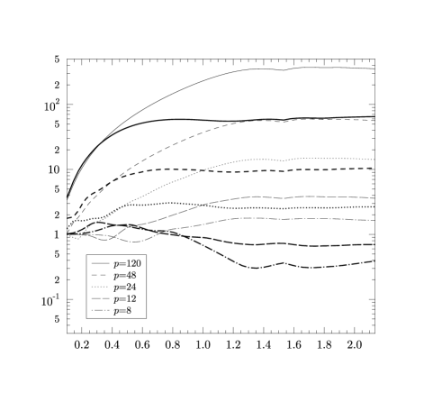
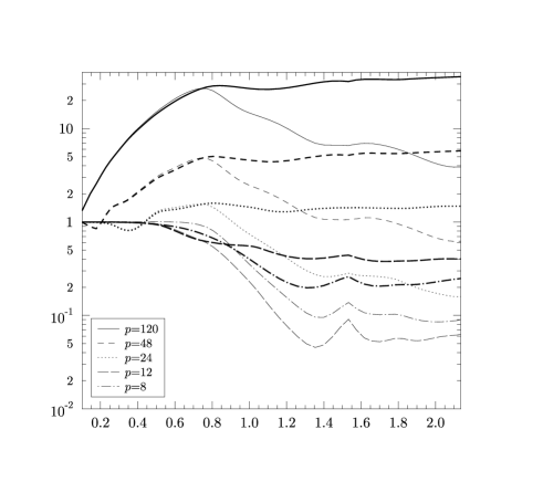
Figure 5: In panel (a) the $S(60^{\circ})$ statistics of the lens spaces $L(p,p/2-1)$ with the observer at $\rho=0$ is compared with the $S(60^{\circ})$ statistics of the homogeneous lens spaces $L(p,1)$. The corresponding results for the lens spaces $L(p,p/2-1)$ with the observer at $\rho=\pi/4$ and for the prism spaces ${\cal D}_{p}$ are shown in panel (b). In both panels the thick lines belong to the lens spaces $L(p,p/2-1)$. In panels (a) and (b) the curves are normalised to the $S(60^{\circ})$ statistics of the projective space ${\cal P}^{3}$. In panel (c), however, the quantity $S(60^{\circ})/p^{2}$ is shown for the lens spaces $L(p,p/2-1)$ at $\rho=\pi/4$ to emphasise the universal behaviour for a large order of the deck group $p$. The $S(60^{\circ})$ statistics of the Poincare dodecahedron ${\cal I}$, the binary octahedral space ${\cal O}$, and the binary tetrahedral space ${\cal T}$ are diagrammed in (d). These three curves are again normalised to the $S(60^{\circ})$ statistics of the projective space ${\cal P}^{3}$. Notice that the scale is different for the vertical axis in all four graphics.

6.2 The large scale CMB anisotropy of lens and prism shaped Voronoi domains

Let us now address the question how the geometry of the Voronoi domain affects the CMB properties. As discussed in the Introduction and in sect. 5, it is most advantageous to consider topologies which possess the same Voronoi domain but with different connections of their faces. The Voronoi domain of $L(p,p/2-1)$ for $\rho=0$ is identical to that of the space $L(p,1)$, and for $\rho=\pi/4$ to that of the prism space ${\cal D}_{p}$. The $S(60^{\circ})$ statistics of the lens shaped Voronoi domains $(\rho=0)$ is shown in figure 5(a) for the group orders $p=8$, 12, 24, 48, and 120. One recognises that the CMB behaviour differs although each pair for a given $p$ of $L(p,p/2-1)$ and $L(p,1)$ possesses the same Voronoi domain. This demonstrates that, in addition to the shape, the connection rules of the Voronoi domains affect the CMB properties. In both cases the $S(60^{\circ})$ statistics growths with the group order $p$. This behaviour could have been anticipated from the increasing asymmetry $\sigma_{\tau}/\langle\tau\rangle$ of the Voronoi domains as shown in figure 3(a) by assuming the validity of the well-proportioned conjecture. In addition, for $\tau_{\hbox{\scriptsize sls}}>0.8$, the $S(60^{\circ})$ statistics takes on larger values for the homogeneous manifold $L(p,1)$ than for the corresponding lens shaped space $L(p,p/2-1)$. Interestingly, this behaviour is reversed for the prism shaped Voronoi domains. In figure 5(b) a comparison of the prism shaped space $L(p,p/2-1)$ at $\rho=\pi/4$ with the prism space ${\cal D}_{p}$ reveals this reversed behaviour for $\tau_{\hbox{\scriptsize sls}}>0.8$. In addition, their behaviour for sufficiently small values of $\tau_{\hbox{\scriptsize sls}}$ is very similar. However, the fact that the curves diverges for $\tau_{\hbox{\scriptsize sls}}\gtrsim 0.8$ demonstrates again that the geometry of the Voronoi domain cannot suffice in order to solely explain the CMB anisotropy suppression. Thus, there are counter-examples to the well-proportioned conjecture.

As figure 3(a) reveals, the shape measure $\sigma_{\tau}/\langle\tau\rangle$ is lower for the prism space ${\cal D}_{8}$ than for ${\cal D}_{12}$. Thus, one would expect that the power in the CMB anisotropy is also lower for ${\cal D}_{8}$. But the reverse behaviour is observed in figures 5(b) and 6(b). Hence, this is a further counter-example to the well-proportioned conjecture.

As just mentioned, the values of the $S(60^{\circ})$ statistics increase with the group order $p$. It turns out that the proportionality is $1/p^{2}$ as shown in figure 5(c) where the quantity $\frac{S_{\cal M}(60^{\circ})}{p^{2}}$ is plotted for the prism shape $L(p,p/2-1)$ at $\rho=\pi/4$. With the exception of the space $L(8,3)$, a convergence of the curves with increasing group order $p$ is revealed. The space $L(8,3)$ at $\rho=\pi/4$ is a special case since it is a spherical Platonic space, see [22]. A similar scaling behaviour occurs at $\rho=0$ where the Voronoi domains possess the shape of a lens. Thus, a universal behaviour emerges at large order $p$ of the deck group.

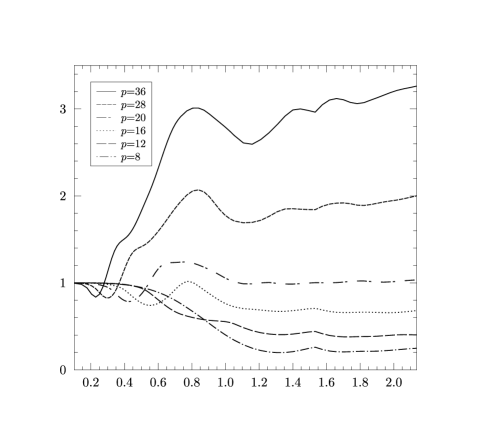
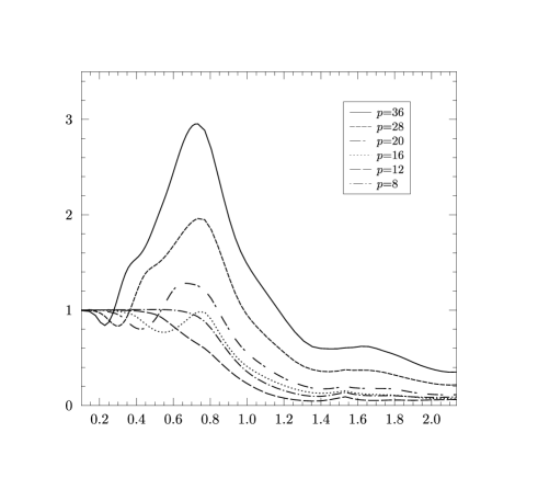
Figure 6: The $S(60^{\circ})$ statistics is compared between models having the same Voronoi domain. The selected group orders are $p=8$, 12, 16, 20, 28, and 36. The panels (a) and (b) refer to the prism shaped domains for $L(p,p/2-1)$ with the observer at $\rho=\pi/4$ and the prism spaces ${\cal D}_{p}$. The CMB correlations of the lens shaped domains of $L(p,p/2-1)$ with the observer at $\rho=0$ and of the lens spaces $L(p,1)$ are displayed in panels (c) and (d).

The $S(60^{\circ})$ statistics of the binary polyhedral spaces ${\cal I}$, ${\cal O}$, and ${\cal T}$ is presented in figure 5(d). This allows the comparison of these well studied models with the multi-connected spaces shown in the other figures. The minimum at $\tau_{\hbox{\scriptsize sls}}\simeq 0.45$ for the Poincaré dodecahedron ${\cal I}$ is the due to the famous CMB correlation suppression at $\Omega_{\hbox{\scriptsize tot}}\simeq 1.02$.

A further interesting detail of the $S(60^{\circ})$ statistics is revealed in figure 6. The figures 6(a) and 6(b) display the CMB behaviour for the prism shaped models $L(p,p/2-1)$ at $\rho=\pi/4$ and ${\cal D}_{p}$, respectively. A comparison of the $S(60^{\circ})$ statistics for the models with $p=36$ (full curve) shows that $L(36,17)$ and ${\cal D}_{36}$ possess for $\tau_{\hbox{\scriptsize sls}}\lesssim 0.7$ a similar statistics but completely different values for larger $\tau_{\hbox{\scriptsize sls}}$. The cosmological interesting minima are below $\tau_{\hbox{\scriptsize sls}}\simeq 0.6$ and, thus, both models give the same statistical description for our Universe. The same trend is seen for all the other group orders $p$. This might be a point in favour of the well-proportioned hypothesis. However, a counter-example is provided by the lens shaped models $L(p,p/2-1)$ at $\rho=0$ and $L(p,1)$ shown in figures 6(c) and 6(d). Despite identical Voronoi domains, their statistics are dissimilar even for small distances $0.1\lesssim\tau_{\hbox{\scriptsize sls}}\lesssim 0.6$. While the homogeneous models $L(p,1)$ have minima comparable to those of the prism spaces, the lens shaped models $L(p,p/2-1)$ at $\rho=0$ have none at all. The latter possess even more CMB anisotropy power than the projective space ${\cal P}^{3}$ for cosmological interesting values of $\tau_{\hbox{\scriptsize sls}}$. For small values of $\tau_{\hbox{\scriptsize sls}}$ the homogeneous lens spaces $L(p,1)$ display lower power of the correlation function $C(\vartheta)$ than the projective space ${\cal P}^{3}$ and the 3-sphere ${\cal S}^{3}$. The minima of the $S(60^{\circ})$ statistics occur between $\tau_{\hbox{\scriptsize sls}}=\pi/p$ and $2\,\pi/p$.

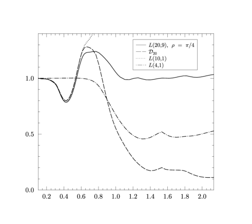
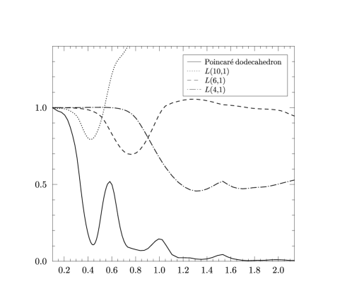
Figure 7: In panel (a) the influence of the cyclic subgroups on the $S(60^{\circ})$ statistics of the prism space ${\cal D}_{20}$ and of the lens space $L(20,9)$ with the observer at $\rho=\pi/4$ is studied. For this purpose also the $S(60^{\circ})$ statistics for the lens spaces $L(10,1)$ and $L(4,1)$ are shown. The analogous influence is studied in panel (b) for the Poincaré dodecahedron. The decomposition of its deck group given in table 2 requires the comparison with the $S(60^{\circ})$ statistics of the lens spaces $L(10,1)$, $L(6,1)$, and $L(4,1)$.

6.3 The role of cyclic subgroups $Z_{p}$ of Clifford translations

The geometrical interpretation of the role of cyclic subgroups of Clifford translations is that such a subgroup determines the gluing rule for two opposing faces of the Voronoi domain. Because Clifford translations shift all points on the 3-sphere ${\cal S}^{3}$ by the same distance, the largest of those subgroups is related to the closest constant distance between such opposing faces which in turn determines the order of the wavelength of a perturbation in that direction and thus the CMB anisotropy suppression. Therefore, the subgroup $Z_{p}$ belonging to the largest value of $p$ is the most interesting from our point of view. Subgroups of the largest subgroup $Z_{p}$, which have a common transfomation direction, are ignored in the following. The origin of a similar or a diverging behaviour for models with an identical Voronoi domain can be understood in terms of these subgroups.

The deck groups $\Gamma$ can possess common subgroups of Clifford translations. The trivial subgroup is the cyclic subgroup $Z_{1}$ which is common to all spherical models. The cyclic subgroup $Z_{2}$ generates the projective space ${\cal P}^{3}$. Since we consider the normalised $\frac{S_{\cal M}(60^{\circ})}{S_{{\cal P}^{3}}(60^{\circ})}$ statistics, the contribution of the subgroup $Z_{2}$ drops out of the curves shown in our figures. Thus, both subgroups are ignored in the following. Since only even group orders $p$ are considered in this paper, the first possible interesting common subgroup is $Z_{4}$. This subgroup of homogeneous translations occurs if the order of the deck group $p$ is a multiple of four. Let us put the focus on the case $p=20$. The CMB anisotropy of the prism shaped models $L(20,9)$ at $\rho=\pi/4$ and ${\cal D}_{20}$ is shown in figure 7(a) together with those of $L(4,1)$ and $L(10,1)$ belonging to the subgroups $Z_{4}$ and $Z_{10}$. The inspection of figure 7(a) reveals that for $\tau_{\hbox{\scriptsize sls}}\lesssim 0.6$ the curves for $L(20,9)$, ${\cal D}_{20}$, and $L(10,1)$ are nearly indistinguishable. This shows that the behaviour for $L(20,9)$ and ${\cal D}_{20}$ is dominated by the common subgroup $Z_{10}$. Omitting $Z_{5}\subset Z_{10}$, since it acts in the same direction as the subgroup $Z_{10}$, the next common subgroup is $Z_{4}$. The anisotropy of $L(4,1)$ differs only for $\tau_{\hbox{\scriptsize sls}}\gtrsim 0.8$ from the projective space ${\cal P}^{3}$. Since the subgroup $Z_{4}$ occurs in the deck groups of $L(20,9)$ and ${\cal D}_{20}$ with different multiplicities, their behaviour splits for those values of $\tau_{\hbox{\scriptsize sls}}$. As listed in table 2, the subgroup $Z_{4}$ occurs in $L(20,9)$ only once whereas the multiplicity of $Z_{4}$ in ${\cal D}_{20}$ is five. Note that the subgroup $Z_{10}$ has in $L(20,9)$ as well as in ${\cal D}_{20}$ the multiplicity one and, therefore, leads to a common behaviour. A diverging behaviour can thus take place when a common cyclic subgroup occurs with different multiplicities with respect to the deck groups.

The homogeneous space $L(20,1)$ possesses as the largest subgroup of Clifford translations the cyclic group $Z_{20}$. This is in contrast to $L(20,9)$ where the subgroup $Z_{20}$ is realised by inhomogeneous translations and largest subgroup of Clifford translations is realised by $Z_{10}$, see table 2. The figures 6(c) and 6(d) display this difference for small values of $\tau_{\hbox{\scriptsize sls}}$.

A subgroup influences the CMB anisotropy when the smallest dimension of its Voronoi domain is at most of the order of the surface of last scattering. Otherwise the surface of last scattering is contained completely inside the Voronoi domain. This requires $\tau_{\hbox{\scriptsize sls}}>\pi/p$ such that a subgroup can modify the CMB. The subgroup with the largest group order determines the CMB anisotropy for the smallest values of $\tau_{\hbox{\scriptsize sls}}$. Since the largest subgroup occurs usually in both spaces with the same multiplicity, i. e. multiplicity one, the common anisotropy is explained in this way. With increasing values of $\tau_{\hbox{\scriptsize sls}}$ the subgroups with decreasing group order influence the CMB. Thus, as long as the common subgroups occur with the same multiplicity, the $S_{\cal M}(60^{\circ})$ statistics of those spaces is very similar. The different behaviour is enforced by the largest subgroup that occurs in both spaces with a different multiplicity. Another possibility is that a subgroup occurs in only one of the two spaces.

manifold ${\cal M}$	# of the cyclic subgroups
	$Z_{20}$	$Z_{10}$	$Z_{8}$	$Z_{6}$	$Z_{4}$
$L(20,1)$	1	-	-	-	-
$L(20,9)$	-	1	-	-	1
${\cal D}_{20}$	-	1	-	-	5
${\cal T}$	-	-	-	4	3
${\cal O}$	-	-	3	4	6
${\cal I}$	-	6	-	10	15

Table 2: The multiplicities of the cyclic subgroups $Z_{p}$, $p=4,6,8,10,20$, of the deck groups $\Gamma$ are listed for the lens space $L(20,1)$, the lens space $L(20,9)$, the prism space ${\cal D}_{20}$, the binary tetrahedral space ${\cal T}$, the binary octahedral space ${\cal O}$, and the Poincaré dodecahedron ${\cal I}$. From the subgroups of Clifford translations acting in the same direction, only the largest independent subgroups are listed in the table. The cyclic subgroups $Z_{p}\subset\Gamma$ of Clifford translations are related to the deck groups of the homogeneous lens spaces $L(p,1)$.

In figure 7(b) the CMB anisotropy of the Poincaré dodecahedron ${\cal I}$ is decomposed in terms of its subgroups. This space provides the best description of the large scale CMB anisotropy with respect to spherical models. Among the subgroups of Clifford translations of the Poincaré dodecahedron ${\cal I}$ are the cyclic groups $Z_{4}$, $Z_{6}$, and $Z_{10}$, see table 2. Consequently, figure 7(b) displays the CMB anisotropies of the homogeneous lens spaces $L(4,1)$, $L(6,1)$, and $L(10,1)$. The famous minimum in the CMB anisotropy of the Poincaré dodecahedron ${\cal I}$ in the range $\tau_{\hbox{\scriptsize sls}}=0.4\dots 0.5$ is due to the subgroup $Z_{10}$ as the comparison with $L(10,1)$ reveals. That the Poincaré dodecahedron possesses a much stronger anisotropy suppression than the $L(10,1)$ space is enforced by the fact that the $Z_{10}$ subgroup in the dodecahedral space has a multiplicity of 6. The second minimum is caused by the subgroup $Z_{6}$ at higher values of $\tau_{\hbox{\scriptsize sls}}$. This subgroup also belongs to the binary octahedral group $O^{\star}$ and the binary tetrahedral group $T^{\star}$. Since it is the largest subgroup of the binary tetrahedral group $T^{\star}$, the binary tetrahedral space ${\cal T}$ has its first minimum at the position of the minimum of $L(6,1)$ as figure 5(d) confirms. The first minimum in the case of the binary octahedral space ${\cal O}$ is dictated by the subgroups $Z_{8}$ and $Z_{6}$, and it is a superposition of those of $L(8,1)$ and $L(6,1)$. In the same way one can also explain why the prism space ${\cal D}_{12}$ displays lower power in the CMB anisotropy than the prism space ${\cal D}_{8}$ for $\tau_{\hbox{\scriptsize sls}}\gtrsim\pi/6$, see figure 6(b). The deck group of the prism space ${\cal D}_{8}$ is composed of three cyclic subgroups $Z_{4}$ which determine the minimum of the $S(60^{\circ})$ statistics. In addition, the deck group $D^{\star}_{12}$ contains a further subgroup $Z_{6}$. Thus, the influence of the additional subgroup $Z_{6}$ within the deck group of the prism space ${\cal D}_{12}$ is the explanation for the lower power of the CMB anisotropy compared to the manifold ${\cal D}_{8}$.

6.4 The transformation behaviour of $\Gamma$ on the sphere $S_{\hbox{\scriptsize sls}}$ of last scattering

The above discussion of the role of the subgroups of Clifford translations explains the similarities of the $S_{\cal M}(60^{\circ})$ statistics for small values of $\tau_{\hbox{\scriptsize sls}}$ as revealed by figures 6(a) and 6(b) which refer to the prism shaped $L(p,p/2-1)$ at $\rho=\pi/4$ and the prism space ${\cal D}_{p}$. This and the distinct behaviour between the lens shaped $L(p,p/2-1)$ at $\rho=0$ and the lens space $L(p,1)$ shown in figures 6(c) and 6(d) can be illuminated from the following point of view. Consider the action of the deck group $\Gamma$ on the sphere $S_{\hbox{\scriptsize sls}}$ of last scattering having a radius $\tau_{\hbox{\scriptsize sls}}$. Every point $x\in S_{\hbox{\scriptsize sls}}$ on this sphere is shifted by a certain distance $d_{n}^{{\cal M}}(\vec{x})$ under the action of a group element $g_{n}\in\Gamma$. Similarities or differences of this transformation behaviour determine whether the $S_{\cal M}(60^{\circ})$ differs or not for not too large values of $\tau_{\hbox{\scriptsize sls}}$. Since there is no direct link between the shape of the Voronoi domain and the transformation structure on $S_{\hbox{\scriptsize sls}}$, the following argument is not directly connected to the well-proportioned hypothesis.

At first the transformation distances are needed. Applying the group elements (13) of the lens space $L(p,q)$ for $\alpha=\epsilon=0$ to a point $\vec{x}$, one gets the points $\vec{x}_{n}$, $n=1,\dots,p$, which are identified with the point $\vec{x}$ on the covering space ${\cal S}^{3}$. The distances $d_{n}^{L(p,q),\rho}(\vec{x})$ between the point $\vec{x}$ and the points $\vec{x}_{n}$ are given by

$$d_{n}^{L(p,q),\rho}(\vec{x})\;=\;\hbox{arccos}\left(\vec{x}\cdot\vec{x}_{n}\right)\hskip 10.0pt,\hskip 10.0ptn=1,\dots,p$$ (45)

$$\hbox{with}\hskip 15.0pt\vec{x}\cdot\vec{x}_{n} = \frac{1}{2}(1-\cos(2\rho))\cos(q\varphi_{n})$$

$$+\frac{1}{2}(1+\cos(2\rho))\cos(\varphi_{n}))$$

$$+\cos(2\rho)(\cos(q\varphi_{n})-\cos(\varphi_{n}))(x_{1}^{2}+x_{2}^{2})$$

$$-\sin(2\rho)(\cos(q\varphi_{n})-\cos(\varphi_{n}))(x_{0}x_{1}+x_{2}x_{3})\hskip 10.0pt,$$

where the special case $\rho=0$ is also discussed in [33]. Here the abbreviation

$$\varphi_{n}\;:=\;2\pi n/p$$ (46)

is introduced. Now we restrict the distances $d_{n}^{{\cal M}}(\vec{x})$ to points $\vec{x}$ lying on the sphere $S_{\hbox{\scriptsize sls}}$ of last scattering. The minimum and the maximum of the distances $d_{n}^{{\cal M}}(\vec{x})$ taken over all points $\vec{x}\in S_{\hbox{\scriptsize sls}}$ are for the lens spaces $L(p,q)$ with the observer at $\rho=0$ given by

$$d_{n,\hbox{\scriptsize min}}^{L(p,q),\rho=0}=\hbox{min}\left[\varphi_{n},\varphi_{\left|p-n\right|}\right]$$ (47)

and

$$d_{n,\hbox{\scriptsize max}}^{L(p,q),\rho=0}=\hbox{arccos}\left(w_{n}\right)$$ (48)

$$\hbox{with}\hskip 20.0ptw_{n}=\cos(\varphi_{n})+\sin^{2}(\tau_{\hbox{\scriptsize sls}})(\cos(q\varphi_{n})-\cos(\varphi_{n}))\hskip 10.0pt.$$

Eq. (48) simplifies for the lens spaces $L(p,p/2-1)$ to

$$d_{n,\hbox{\scriptsize max}}^{L(p,p/2-1),\rho=0}=\left\{\begin{array}[]{ll}\hbox{arccos}\left(w_{n}\right)&:n\;\;\hbox{odd}\\ d_{n,\hbox{\scriptsize min}}^{L(p,p/2-1),\rho=0}&:n\;\;\hbox{even}\end{array}\right.$$ (51)

$$\hbox{with}\hskip 20.0ptw_{n}=\cos(\varphi_{n})-2\sin^{2}(\tau_{\hbox{\scriptsize sls}})\sin((p/4-1)\varphi_{n})\hskip 10.0pt.$$

For the other observer position $\rho=\pi/4$ one gets for $L(p,p/2-1)$

$$d_{n,\hbox{\scriptsize min}}^{L(p,p/2-1),\rho=\pi/4}=\left\{\begin{array}[]{ll}\hbox{min}_{\{i=1,2\}}\left[\hbox{arccos}\left(w^{i}_{n}\right)\right]&:n\;\;\hbox{odd},\;\;\tau_{\hbox{\scriptsize sls}}\leq\pi/4\\ \hbox{min}\left[\varphi_{n},\varphi_{\left|p/2-n\right|},\varphi_{\left|p-n\right|}\right]&:n\;\;\hbox{odd},\;\;\tau_{\hbox{\scriptsize sls}}>\pi/4\\ \hbox{min}\left[\varphi_{n},\varphi_{\left|p-n\right|}\right]&:n\;\;\hbox{even}\end{array}\right.\hskip 10.0pt$$ (52)

and

$$d_{n,\hbox{\scriptsize max}}^{L(p,p/2-1),\rho=\pi/4}=\left\{\begin{array}[]{ll}\hbox{max}_{\{i=1,2\}}\left[\hbox{arccos}\left(w^{i}_{n}\right)\right]&:n\;\;\hbox{odd},\;\;\tau_{\hbox{\scriptsize sls}}\leq\pi/4\\ \hbox{max}\left[\varphi_{n},\varphi_{\left|p/2-n\right|},\varphi_{\left|p-n\right|}\right]&:n\;\;\hbox{odd},\;\;\tau_{\hbox{\scriptsize sls}}>\pi/4\\ d_{n,\hbox{\scriptsize min}}^{L(p,p/2-1),\rho=\pi/4}&:n\;\;\hbox{even}\end{array}\right.$$ (53)

with

$$w^{1,2}_{n} = \cos(n\pi/2)\cos((p/4-1)\varphi_{n})$$

$$\pm 2\sin(n\pi/2)\sin((p/4-1)\varphi_{n})\sin(\tau_{\hbox{\scriptsize sls}})\cos(\tau_{\hbox{\scriptsize sls}})\hskip 10.0pt.$$

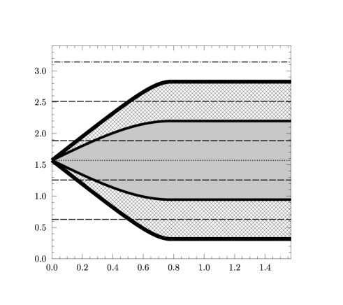
Figure 8: The transformation distances $d_{n}^{{\cal M}}(\vec{x})$ for points $\vec{x}\in S_{\hbox{\scriptsize sls}}$ are plotted for the manifolds $L(20,1)$, ${\cal D}_{20}$, and $L(20,9)$ with the observer position at $\rho=0$ and at $\rho=\pi/4$. Since $L(20,9)$ for $\rho=\pi/4$ and ${\cal D}_{20}$ have the same prism geometry of the Voronoi domain, one has to compare the panels (a) and (b). The panel pair (c) and (d) is devoted to the lens shaped case. The inhomogeneous manifold $L(20,9)$ possesses a wide distribution of values of $d_{n}^{{\cal M}}(\vec{x})$ for $n=1$, 3, 7, 9, 11, 13, 17, and 19 which are depicted by the grey and shaded bands.

The elements of the deck group of a homogeneous lens space $L(p,1)$ transform all points on the 3-sphere by the same distance since they are all Clifford translations. So one gets independent of $\vec{x}$ the distance

$$d_{n}^{L(p,1)}(\vec{x})=d_{n,\hbox{\scriptsize min}}^{L(p,1)}=d_{n,\hbox{\scriptsize max}}^{L(p,1)}=\hbox{min}\left[\varphi_{n},\varphi_{\left|p-n\right|}\right]\hskip 10.0pt.$$ (55)

This general property of homogeneous manifolds occurs in the inhomogeneous case only for special cases. The eqs. (51) and (53) show that the property $d_{n,\hbox{\scriptsize max}}^{L(p,p/2-1),\rho}=d_{n,\hbox{\scriptsize min}}^{L(p,p/2-1),\rho}=d_{n}^{L(p,p/2-1),\rho}(\vec{x})$ is only obtained for even values of $n$ which correspond to the cyclic subgroup $Z_{p/2}$ of the homogeneous lens space $L(p/2,1)$. Eqs. (52) and (53) lead for $n=p/4$ and $n=3p/4$ to the simple result $d_{n,\hbox{\scriptsize max}}^{L(p,p/2-1),\rho}=d_{n,\hbox{\scriptsize min}}^{L(p,p/2-1),\rho}=\pi/2$. This distance belongs to two group elements of the deck group $Z_{4}$ which generates the homogeneous lens space $L(4,1)$.

The deck group $D^{\star}_{p}$ of the homogeneous prism space ${\cal D}_{p}$ contains the cyclic subgroup $Z_{p/2}$ and $p/4$ times the cyclic subgroup $Z_{4}$. For this reason the distances $d_{n}^{{\cal D}_{p}}(\vec{x})$ are given by

$$d_{n}^{{\cal D}_{p}}(\vec{x})=d_{n,\hbox{\scriptsize min}}^{{\cal D}_{p}}=d_{n,\hbox{\scriptsize max}}^{{\cal D}_{p}}=\left\{\begin{array}[]{ll}\hbox{min}\left[\varphi_{n},\varphi_{\left|p-n\right|}\right]&:n\;\;\hbox{even}\\ \pi/2&:n\;\;\hbox{odd}\end{array}\right.\hskip 6.0pt.$$ (56)

The distance $d_{n}^{{\cal D}_{p}}(\vec{x})=\pi/2$ results from the $p/2$ group elements $g_{n}$ of the $p/4$ cyclic subgroups $Z_{4}$.

The distances $d_{n}^{{\cal M}}(\vec{x})$ according to the formulae (47) to (56) are shown in figure 8 for the same topologies as in figure 6 for the special case $p=20$. The homogeneous spaces ${\cal D}_{20}$ and $L(20,1)$ have distances $d_{n}^{{\cal M}}(\vec{x})$ independent of $\tau_{\hbox{\scriptsize sls}}$ which are shown as horizontal lines in figures 8(b) and 8(d). The index $n$ of the distance $d_{n}^{{\cal M}}(\vec{x})$ is also stated in figure 8. The case for the inhomogeneous space $L(20,9)$ is more involved, since only distances $d_{n}^{{\cal M}}(\vec{x})$ with an even value of $n$ are $\tau_{\hbox{\scriptsize sls}}$ independent. For odd $n$ the distance $d_{n}^{{\cal M}}(\vec{x})$ can extend over the interval $[d_{n,\hbox{\scriptsize min}},d_{n,\hbox{\scriptsize max}}]$ which is shown as the bands in figures 8(a) and 8(c). A comparison of figure 8(a) with 8(b) shows that for $\tau_{\hbox{\scriptsize sls}}\lesssim 0.5$ the smallest distances $d_{n}^{{\cal M}}(\vec{x})$ belonging to $n=2$ and $n=18$ are identical for $L(20,9)$ at $\rho=\pi/4$ and ${\cal D}_{20}$. Since the distance $d_{n}^{{\cal M}}(\vec{x})$ determines the maximal wavelength of a perturbation along the transformation direction of $g_{n}$, the smallest distance is most responsible for the suppression of the large angular CMB anisotropy. Since it is equal for both spaces for $\tau_{\hbox{\scriptsize sls}}\lesssim 0.5$, the CMB anisotropy behaviour is almost the same. On the other hand, the inhomogeneous transformations $n=1,9,11,19$ belong for $\tau_{\hbox{\scriptsize sls}}\gtrsim 0.5$ to the smallest transformation distance, and the diverging CMB properties are also explained. The situation is different for the spaces $L(20,9)$ at $\rho=0$ and $L(20,1)$ shown in figures 8(c) and 8(d). Here, the smallest distance $d_{n}^{{\cal M}}(\vec{x})$ belongs to $n=1$ and $n=19$ and is independent of $\tau_{\hbox{\scriptsize sls}}$ for $L(20,1)$, of course. However, for the inhomogeneous space $L(20,9)$ at $\rho=0$, the $d_{n}^{{\cal M}}(\vec{x})$ are distributed towards larger values, and there are thus directions with a less pronounced CMB anisotropy suppression. This distinction already happens at very small values of $\tau_{\hbox{\scriptsize sls}}$ as reflected in figures 6(c) and 6(d). The transformation properties of the deck group $\Gamma$ on the sphere $S_{\hbox{\scriptsize sls}}$ of last scattering determine the CMB anisotropy in this way. Since they are not related to the shape of the Voronoi domain, their consequences are independent of the well-proportioned conjecture.

Figure 9: The variation of the $S(60^{\circ})$ statistics with respect to the observer position parametrised by $\rho$ is shown for the lens spaces $L(8,3)$, $L(12,5)$, $L(20,9)$, and $L(32,15)$. In all four diagrams the $S(60^{\circ})$ statistics with the largest values belongs to the lens shaped geometry of the Voronoi domain ($\rho=0$).

6.5 The CMB anisotropy for general observer positions $\rho$

Up to now, only two special positions of the observer in the inhomogeneous spaces $L(p,p/2-1)$ have been discussed since the two positions at $\rho=0$ and $\rho=\pi/4$ lead to Voronoi domains identical to two other homogeneous spaces. To close this gap, the variation of the CMB anisotropy with respect to the observer position $\rho$ is shown in figure 9 for the four spaces $L(8,3)$, $L(12,5)$, $L(20,9)$, and $L(32,15)$. The $S(60^{\circ})$ statistics is shown for 12 values of $\rho$ for these spaces. The band width generated by these twelve curves shows how strong the CMB properties vary as a function of the observer position. It turns out that the largest CMB anisotropy belongs to the lens shaped Voronoi domain $(\rho=0)$ in all four cases. For sufficiently large spheres of last scattering $\tau_{\hbox{\scriptsize sls}}=0.8\dots 1.0$, the prism shaped Voronoi domains $(\rho=\pi/4)$ possess the smallest CMB anisotropy. For CMB spheres with smaller $\tau_{\hbox{\scriptsize sls}}$ other values of $\rho$ can lead to an even smaller CMB anisotropy and thus to a better description of the CMB observations. It is worthwhile to note that for other spaces $L(p,q)$ with $q\neq p/2-1$ and $q\neq 1$ the situation is more involved such that this simple behaviour does not emerge in the general case. This will be the topic of a future work.

Figure 10: The variation of the $S(60^{\circ})$ statistics with respect to the observer position parametrised by $\rho$ is shown for the lens spaces $L(8,3)$ and $L(20,9)$ for four values of $\tau_{\hbox{\scriptsize sls}}$. In addition, the shape measure $\sigma_{\tau}/\langle\tau\rangle$ for these two manifolds is given as a solid curve.

Now, we return to the possible link between the geometry of the Voronoi domain and the large scale CMB anisotropy suppression. In sect. 5 the relative variation $\sigma_{\tau}/\langle\tau\rangle$ is introduced as a measure of the sphericity of the Voronoi domain. The smaller its value is, the more well-proportioned is the Voronoi domain, which should in turn lead to a stronger anisotropy suppression. In figure 9 the $S(60^{\circ})$ statistics is already shown for twelve observer positions as a function of the cosmological parameters encoded by $\tau_{\hbox{\scriptsize sls}}$. But in figure 10 the $S(60^{\circ})$ statistics of $L(8,3)$ and $L(20,9)$ is shown as a function of $\rho$ such that it can be compared to the shape measure $\sigma_{\tau}/\langle\tau\rangle$ (solid curve). The shape measure is independent of the cosmological parameters and has a minimum for the prism shaped Voronoi domain, i. e. for $\rho=\pi/4$. As can be seen in figure 10, there are values of $\tau_{\hbox{\scriptsize sls}}$ for which the minimum in the $S(60^{\circ})$ statistics does not occur at $\rho=\pi/4$. Thus, Voronoi domains that are more oddly shaped than the prism produce less CMB anisotropy on large angular scales. This again demonstrates that the geometry of the Voronoi domain is only partially responsible for the anisotropy suppression.

7 Summary and Discussion

The main motivation for cosmic topology is the low power of the CMB anisotropy that is observed at large angular scales in the data of COBE [1] and WMAP [2]. The large-scale behaviour is revealed by the temperature 2-point correlation function $C(\vartheta)$ and could be at variance with the $\Lambda$CDM concordance model based on a space with infinite volume as emphasised by [32, 21, 34]. The reality of this discordance is, however, questioned in [35, 36] where a reconstruction algorithm is used for the masked sky regions. It turns out that significant power arises just in those reconstructed regions. Using only save data from sky regions, which are not masked, a very low temperature correlation is obtained for angles $\vartheta\gtrsim 60^{\circ}$. The papers [37, 38] conclude that it is very likely that the low power at large angles is real. And if the low power behaviour is not a statistical fluke, models, which naturally have few CMB correlations on large scales, deserve a further investigation.

Because of the large number of topological spaces, it would be desirable to have a guiding principle that reduces the number of possibilities. It is claimed in [20] that well proportioned manifolds can describe the low power of the observed CMB, but the well-proportioned conjecture is not quantified there. To quantify this conjecture by a shape measure, the variance of the spherical distance to the surface of the fundamental cell defined as the Voronoi domain is introduced in sec. 5. This variance is small for almost spherical Voronoi domains and large for oddly shaped ones. The lens spaces $L(p,p/2-1)$ are at the focus of this paper since they provide inhomogeneous spaces so that the shape of the Voronoi domain depends on the position of the observer. They are thus predestined for a test of the well-proportioned conjecture. Furthermore, for two special positions of the observer, they have Voronoi domains identical to those of the homogeneous $L(p,1)$ and ${\cal D}_{p}$ spaces.

The first observer position is characterised by $\rho=0$ and results in a lens shaped Voronoi domain. Therefore, the manifold $L(p,p/2-1)$ at $\rho=0$ has the same value for the shape measure as the homogeneous lens space $L(p,1)$. The CMB anisotropies at large angular scales of both are compared in sec. 6.2, and it turns out that the correlations of the CMB of $L(p,p/2-1)$ at $\rho=0$ and of $L(p,1)$ are different contrary to the well-proportioned conjecture.

The second observer position is at $\rho=\pi/4$, in which case the Voronoi domain of $L(p,p/2-1)$ is prism shaped and identical to that of the prism space ${\cal D}_{p}$. For these two topologies, the $S(60^{\circ})$ statistics of the CMB also diverges at least for large distances $\tau_{\hbox{\scriptsize sls}}\gtrsim 0.8$ to the surface of last scattering. Thus, a second counter-example to the well-proportioned hypothesis is found. For this reason, the conjecture does not provide a save criterion for the decision whether a multi-connected universe is an eligible candidate for our Universe or not.

Interestingly, for small values of $\tau_{\hbox{\scriptsize sls}}$, the prism shaped universe $L(p,p/2-1)$ at $\rho=\pi/4$ does behave almost identical to the prism space ${\cal D}_{p}$ with respect to the statistical behaviour of the CMB anisotropies. This similarity can be traced back to the largest common cyclic subgroup $Z_{p}$ of Clifford translations that is contained in their deck groups as outlined in sec. 6.3. If that subgroup occurs in both spaces with the same multiplicity, the CMB anisotropies turn out to be similar. Conversely, if it occurs with different multiplicities in the two spaces or in only one of them, the CMB properties are different. Furthermore, the order $p$ of the cyclic subgroup $Z_{p}$ is linked to the scale on which the power of the CMB anisotropy is suppressed. The larger the order $p$, the smaller distances $\tau_{\hbox{\scriptsize sls}}$ are necessary for a CMB anisotropy suppression and this translates to smaller densities $\Omega_{\hbox{\scriptsize tot}}>1$. Thus, almost flat cosmological models can be obtained when this subgroup possesses a sufficient high group order $p$. The distinct CMB statistics of the prism shaped universes for large distances $\tau_{\hbox{\scriptsize sls}}$ as well as those of the lens shaped universes is explained by such cyclic subgroups.

In addition to the lens and prism shaped fundamental cells, sec. 6.3 also analyses the minima of the $S(60^{\circ})$ statistics of the three binary polyhedral spaces ${\cal T}$, ${\cal O}$, and ${\cal I}$ in terms of subgroups. The superior behaviour of the Poincaré dodecahedron ${\cal I}$ is due to the sixfold occurrence of the $Z_{10}$ subgroup of Clifford translations.

The dissimilar CMB behaviour of topologies sharing the same Voronoi domain is evidently rooted in the transformation properties of the deck groups on the sphere $S_{\hbox{\scriptsize sls}}$ of last scattering. In sec. 6.4 the translation distances for points on $S_{\hbox{\scriptsize sls}}$ of the elements of the deck group are compared between homogeneous and inhomogeneous spaces. In those cases where the smallest translation distances are the same between two spaces, a similar $S(60^{\circ})$ statistics is observed and vice versa. This provides a complementary picture to the cyclic subgroups.

Although the main topic of this paper is the study of CMB statistics of lens and prism shaped Voronoi domains, sec. 6.5 shows, how the CMB properties vary by moving the observer through the $L(p,q)$ space. This demonstrates the large range of variation for a fixed set of cosmological parameters within a given manifold. The comparison with the shape measure $\sigma_{\tau}/\langle\tau\rangle$ shows that there are examples where more oddly shaped Voronoi domains exhibit less correlations in the CMB power contrary to the well-proportioned conjecture.

Summarising, one concludes that the CMB behaviour results from complex interwoven ingredients such that an individual analysis of topological spaces is necessary in order to deliver a judgement whether a topology leads to suitable CMB properties.

References

References

- [1] G. Hinshaw et al., Astrophys. J. Lett. 464, L25 (1996).
- [2] D. N. Spergel et al., Astrophys. J. Supp. 148, 175 (2003), astro-ph/0302209.
- [3] M. Lachièze-Rey and J.-P. Luminet, Physics Report 254, 135 (1995).
- [4] J.-P. Luminet and B. F. Roukema, Topology of the Universe: Theory and Observation, in NATO ASIC Proc. 541: Theoretical and Observational Cosmology, p. 117, 1999, astro-ph/9901364.
- [5] J. Levin, Physics Report 365, 251 (2002).
- [6] M. J. Rebouças and G. I. Gomero, Braz. J. Phys. 34, 1358 (2004), astro-ph/0402324.
- [7] J.-P. Luminet, The Shape and Topology of the Universe, in Proceedings of the conference ”Tessellations: The world a jigsaw”, Leyden (Netherlands), March 2006, 2008, arXiv:0802.2236 [astro-ph].
- [8] E. Gausmann, R. Lehoucq, J.-P. Luminet, J.-P. Uzan, and J. Weeks, Class. Quantum Grav. 18, 5155 (2001).
- [9] J.-P. Luminet, J. R. Weeks, A. Riazuelo, R. Lehoucq, and J. Uzan, Nature 425, 593 (2003).
- [10] B. F. Roukema, B. Lew, M. Cechowska, A. Marecki, and S. Bajtlik, Astron. & Astrophy. 423, 821 (2004), arXiv:astro-ph/0402608.
- [11] R. Aurich, S. Lustig, and F. Steiner, Class. Quantum Grav. 22, 2061 (2005), arXiv:astro-ph/0412569.
- [12] J. Gundermann, astro-ph/0503014 (2005).
- [13] R. Aurich, S. Lustig, and F. Steiner, Class. Quantum Grav. 22, 3443 (2005), arXiv:astro-ph/0504656.
- [14] R. Aurich, S. Lustig, and F. Steiner, Mon. Not. R. Astron. Soc. 369, 240 (2006), arXiv:astro-ph/0510847.
- [15] S. Lustig, Mehrfach zusammenhängende sphärische Raumformen und ihre Auswirkungen auf die Kosmische Mikrowellenhintergrundstrahlung, PhD thesis, Universität Ulm, 2007, Verlag Dr. Hut, München (2007).
- [16] B. S. Lew and B. F. Roukema, Astron. & Astrophy. 482, 747 (2008), arXiv:0801.1358 [astro-ph].
- [17] B. F. Roukema, Z. Buliński, A. Szaniewska, and N. E. Gaudin, Astron. & Astrophy. 486, 55 (2008), arXiv:0801.0006 [astro-ph].
- [18] B. F. Roukema and T. A. Kazimierczak, Astron. & Astrophy. 533, A11 (2011), arXiv:1106.0727 [astro-ph.CO].
- [19] J.-P. Uzan, A. Riazuelo, R. Lehoucq, and J. Weeks, Phys. Rev. D 69, 043003 (2004), astro-ph/0303580.
- [20] J. Weeks, J.-P. Luminet, A. Riazuelo, and R. Lehoucq, Mon. Not. R. Astron. Soc. 352, 258 (2004), astro-ph/0312312.
- [21] C. J. Copi, D. Huterer, D. J. Schwarz, and G. D. Starkman, Mon. Not. R. Astron. Soc. 399, 295 (2009), arXiv:0808.3767 [astro-ph].
- [22] R. Aurich, P. Kramer, and S. Lustig, Physica Scripta 84, 055901 (2011), arXiv:1107.5214 [astro-ph.CO].
- [23] A. R. Edmonds, Drehimpulse in der Quantenmechanik (Biblographisches Institut, Mannheim, 1964).
- [24] M. Lachièze-Rey, J. Phys. A: Math. Gen. 37, 5625 (2004).
- [25] R. Lehoucq, J.-P. Uzan, and J. Weeks, Kodai Math. J. 26, 119 (2003), math.SP/0202072.
- [26] R. Lehoucq, J. Weeks, J. Uzan, E. Gausmann, and J.-P. Luminet, Class. Quantum Grav. 19, 4683 (2002), astro-ph/0205009.
- [27] J. Weeks, Class. Quantum Grav. 23, 6971 (2006), math.SP/0502566.
- [28] T. Risbo, Journal of Geodesy 70, 383 (1996).
- [29] P. Kramer, Class. Quantum Grav. 27, 095013 (2010).
- [30] A. Ikeda, Kodai Math. J. 18, 57 (1995).
- [31] M. P. Bellon, Class. Quantum Grav. 23, 7029 (2006), arXiv:astro-ph/0602076.
- [32] R. Aurich, H. S. Janzer, S. Lustig, and F. Steiner, Class. Quantum Grav. 25, 125006 (2008), arXiv:0708.1420 [astro-ph].
- [33] B. Mota, G. I. Gomero, M. J. Rebouças, and R. Tavakol, Class. Quantum Grav. 21, 3361 (2004), arXiv:astro-ph/0309371.
- [34] C. J. Copi, D. Huterer, D. J. Schwarz, and G. D. Starkman, Adv. Astron. 2010, 847541 (2010), arXiv:1004.5602 [astro-ph.CO].
- [35] G. Efstathiou, Y.-Z. Ma, and D. Hanson, Mon. Not. R. Astron. Soc. 407, 2530 (2010), arXiv:0911.5399 [astro-ph.CO].
- [36] C. L. Bennett et al., arXiv:1001.4758 [astro-ph.CO] (2010).
- [37] R. Aurich and S. Lustig, Mon. Not. R. Astron. Soc. 411, 124 (2011), arXiv:1005.5069 [astro-ph.CO].
- [38] C. J. Copi, D. Huterer, D. J. Schwarz, and G. D. Starkman, (2011), arXiv:1103.3505 [astro-ph.CO].