Universal dynamical phase diagram of lattice spin models and strongly correlated ultracold atoms in optical lattices.

Abstract

We study semiclassical dynamics of anisotropic Heisenberg models in two and three dimensions. Such models describe lattice spin systems and hard core bosons in optical lattices. We solve numerically Landau-Lifshitz type equations on a lattice and show that in the phase diagram of magnetization and interaction anisotropy, one can identify several distinct regimes of dynamics. These regions can be distinguished based on the character of one dimensional solitonic excitations, and stability of such solitons to transverse modulation. Small amplitude and long wavelength perturbations can be analyzed analytically using mapping of non-linear hydrodynamic equations to KdV type equations. Numerically we find that properties of solitons and dynamics in general remain similar to our analytical results even for large amplitude and short distance inhomogeneities, which allows us to obtain a universal dynamical phase diagram. As a concrete example we study dynamical evolution of the system starting from a state with magnetization step and show that formation of oscillatory regions and their stability to transverse modulation can be understood from the properties of solitons. In regimes unstable to transverse modulation we observe formation of lump type solutions with modulation in all directions. We discuss implications of our results for experiments with ultracold atoms.

Motivation. Understanding nonequilbrium quantum dynamics of many-body systems is an important problem in many areas of physics. The most fundamental challenge facing this field is identifying emergent collective phenomena, which should lead to universality and common properties even in systems which do not have identical microscopic Hamiltonians. We know that in equilibrium many-body systems typically fall within certain universality classes. Basic examples are states with spontaneously broken symmetries such as BEC of bosons and superfluid paired phases of fermionsGiorgini2008 ; Dalfovo1999 , Fermi liquid states of electrons and interacting ultracold fermionsShankar1994 ; Nascimbene2010 . We have numerous examples of emergent universal properties of classical systems driven out of equilibrium (see ref. Cross1993 for a review). However very few examples of collective behavior of coherent quantum evolution of many-body systems, which can be classified as exhibiting emergent universality, are known (several recently studied examples can be found in refs Kinoshita2006 ; Moeckel2008 ; Rigol2008 ; Barmettler2009 ; Polkovnikov2011 ; Schneider ; Gring2011 ) The main result of this paper is demonstration of the universality of semiclassical dynamics of lattice spin systems and strongly interacting bosons in two and three dimensions, summarized in the phase diagram in Fig. 1.

Figure 1: Dynamical phase diagram of the anisotropic Heisenberg model (1) for initial states with finite magnetization in the XY plane. Vertical axis labels magnetization for spin models and density for hard-core bosons on a lattice. Regions I, II correspond to easy plane anisotropy of the Hamiltonian, linearized collective modes are of the hyperbolic type. Regions III correspond to easy axis anisotropy, linearized collective modes are of the elliptic type. Special lines $J_{z}/J_{\perp}=1$ and $m_{z}=\pm 1$ all have linearized collective modes of parabolic type. Region I₊ has particle solitons unstable to transverse modulation. Region I_- has hole solitons unstable to transverse modulation. Region II₊ has hole solitons stable to transverse modulation. Region I_- has particle solitons stable to transverse modulation.

In addition to fundamental conceptual importance, our study has strong experimental motivation. Rapid progress of experiments with ultracold atoms in optical lattices makes it possible to create well controlled realizations of systems that we discuss Bloch2008 ; Lewenstein2007a . Tunability of such systems, nearly perfect isolation from the environment, and a rich toolbox of experimental probes, including the possibility of single site resolution Nelson2007 ; Gemelke2009 ; Sherson2010a ; Bakr2010a , makes them excellent candidates for exploring nonequilibrium quantum dynamics (see Polkovnikov2011 ; Lamacrafta and references therein). Several intriguing nonequilibrium phenomena have been demonstrated recently in ensembles of ultracold atoms, including collapse and revival of coherenceBloch2002 , absence of relaxation in nearly integrable systemsKinoshita2006 , exponential slowdown of relaxation in systems with strong mismatch of excitation energiesStrohmaier2010 , anomalous diffusionSchneider , prethermalizationGring2011 , many-body Landau-Zener transitions Chen2010 , light-cone spreading of correlations in a many-body systemCheneau2011 .

Model. In this paper we study non-equilibrium dynamics of lattice spin models and strongly correlated bosons in optical lattices. Our starting point is the anisotropic Heisenberg model

$${\cal H}_{\rm AH}=-J_{\perp}\sum_{\langle ij\rangle}\left(\sigma_{i}^{x}\sigma_{j}^{x}+\sigma_{i}^{y}\sigma_{j}^{y}\right)-J_{z}\sum_{\langle ij\rangle}\sigma_{i}^{z}\sigma_{j}^{z}$$ (1)

where $\sigma^{a}$ are Pauli matrices. Anisotropic Heisenberg models with tunable interactions can be realized with two component Bose mixtures in spin dependent optical latticesDuan2003 ; Kuklov2003 ; Altman2003 ; Trotzky2008 . Hamiltonian (1) also describes spinless bosons in the regime of infinitely strong on-site repulsionBatrouni1995 . In this case states $|\downarrow\rangle$ and $|\uparrow\rangle$ correspond to states with zero and one boson per site respectively, $J_{\perp}$ is the tunneling strength, and $J_{z}$ is the strength of the nearest neighbor repulsion. For atoms with contact interaction and confined to the lowest Bloch band $J_{z}=0$. Non-local interactions can be present for atoms in higher Bloch bandsScarola2005 and polar moleculesLahaye2009 .

Semiclassical equations of motion can be understood either as the lattice version of Landau-Lifshitz equations or as dynamics in the manifold of variational states $|\Psi(t)\rangle=\prod_{i}[\sin{\theta_{i}\over 2}e^{-i\varphi_{i}/2}|\downarrow\rangle_{i}+\cos{\theta_{i}\over 2}e^{i\varphi_{i}/2}|\uparrow\rangle_{i}]$, where all $\theta_{i}$ and $\varphi_{i}$ are independent functions of time ( see supplementary material and ref. Demler2011a ). It is convenient to introduce parametrization

$\sin{\theta_{i}\over 2}=({1-z_{i}\over 2})^{1/2}$, $\cos{\theta_{i}\over 2}=({1+z_{i}\over 2})^{1/2}$ , $e^{i\varphi_{i}}={x_{i}+iy_{i}\over{(x_{i}^{2}+y_{i}^{2}})^{1/2}}$, then semiclassical dynamical equations are given by

$$\begin{array}[]{c}{\dot{x}_{i}}\,\,=\,\,4\,J_{\perp}\,z_{i}\,\left(y_{i+1}+y_{i-1}\right)\,-\,4\,J_{z}\,y_{i}\,\left(z_{i+1}+z_{i-1}\right)\cr{\dot{y}_{i}}\,\,=\,\,-\,4\,J_{\perp}\,z_{i}\,\left(x_{i+1}+x_{i-1}\right)\,+\,4\,J_{z}\,x_{i}\,\left(z_{i+1}+z_{i-1}\right)\cr{\dot{z}_{i}}\,=\,4\,J_{\perp}\,\left(y_{i}\,x_{i+1}\,-\,x_{i}\,y_{i+1}\,+\,y_{i}\,x_{i-1}\,-\,x_{i}\,y_{i-1}\right)\end{array}$$ (2)

Note that variables $(x_{i},y_{i},z_{i})$ reside on a sphere. Specifying $x_{i}^{2}\,+\,y_{i}^{2}\,+\,z_{i}^{2}\,=1$ in the beginning of the evolution will preserve this condition at all times.

We consider dynamics in a state with finite magnetization in the $XY$ plane (superfluid phase for hard core bosons), where close to equilibrium dynamics is determined by the Bogoliubov (Goldstone) mode. Considerable difference between the nonlinear hydrodynamics of hard core bosons on a lattice and the more familiar GP model was observed in the numerical study of solitary waves in ref. Balakrishnan2009 (for a discussion of solitons in systems of ultracold atoms in the regime where GP equation applies see refs. Burger1999 ; Johansson1999 ; Denschlag2000 ; Trombettoni2001 ; Strecker2002 ; Khaykovich2002 ; Baizakov2003 ; Kevrekidis2003 ; Ahufinger2004 ; Eiermann2004 ; Becker2008 ; Scott2011 ). Additional evidence for the special character of solitons in systems of strongly correlated lattice bosons came from the analytical study in Ref. Demler2011a , which extended linear hydrodynamics to include the first non-linear term and the first dispersion correction to the long wavelength expansion and showed that solitons were of the KdV type. In this paper we derive a full phase diagram of semiclassical dynamics of (1) for initial states with finite magnetization in the XY plane. Our approach relies on combining analytical results describing small density perturbations Demler2011a with numerical studies of equations (2) describing dynamics of large amplitude modulations.

Phase diagram. Hyperbolic, elliptic, and parabolic regimes. The main results of our analysis are summarized in fig. 1. Firstly there is fundamental difference between elliptic and hyperbolic regions in the character of linearized equations of motion. The hyperbolic regime (hyperbolic regions I and II in fig. 1) corresponds to the easy plane anisotropy of the Hamiltonian. If we start with initial state that has finite magnetization in the XY plane, we find collective modes with linear dispersion, $\omega\propto|q|$, which describe Bogoliubov (Goldstone) modes. In the elliptic regime we have easy axis anisotropy: lowest energy configuration should have full polarization along the z-axis, $m=\pm 1$. However our initial state has magnetic order in the XY plane. Thus we find unstable collective modes with imaginary frequency ${\it Im}\,\omega\propto\pm|q|$. This corresponds to the dynamical instability in which small density fluctuations grow in time exponentially at short time scales. There are also several special lines on the phase diagram 1: the SO(3) symmetric Heisenberg model with $J_{z}=J_{\perp}$ and fully polarized regimes $m=\pm 1$ (fully occupied or empty regimes for spinless bosons). In all of these cases collective modes have quadratic dispersion, i.e. linearized equations of motion are of the parabolic type.

Hyperbolic regime. Solitons. Hyperbolic regions I and II are differentiated further according to the character of solitonic excitations. In region I₊ we find particle-like one dimensional solitons, which are unstable to modulation in the transverse directions. In region I_- we find hole-like one dimensional solitons unstable to transverse modulations. In regions II_± we find particle and hole-like solitons stable to transverse modulation. Lines ${\rm IV}_{1}$ and ${\rm IV}_{2}$ correspond to two different regimes of the mKdV equation. Both hole and particle-type soliton solutions can be found on the line ${\rm IV}_{2}$. Both types of solitons are suppressed close to the line ${\rm IV}_{1}$.

In the limit of small amplitude and long wavelength inhomogeneities non-linear hydrodynamic equations (2) can be mapped to KdV type equations and solitons can be studied analytically (see supplementary material and ref. Demler2011a ). This analysis can be used to obtain explicit expressions for boundaries of different regimes in fig. 1. In the general case of large amplitude inhomogeneities one needs to solve lattice equations (2) numerically. Surprisingly we find that in even for large amplitude solitons, their properties, including stability to transverse fluctuations, are consistent with small amplitude solitons. Hence the phase diagram in fig. 1 is generic.

While we can not present all of our numerical results, we provide examples, which demonstrate properties of large amplitude solitons. Fig. 2 shows particle- and hole-type solitons in regions I₊ and II₊ respectively. These specific solutions were chosen arbitrarily from a plethora of solitons with different amplitudes and velocities, which can be found in the system for the same values of microscopic parameters. In these specific examples only one dimensional variation of parameters were considered when solving lattice equations (2). The possibility of transverse modulation of one dimensional solitons in two dimensional systems is considered in figures 3, 4. These figures contrast stable and unstable regimes. In the stable regime II₊ transverse modulation does not lead to any dramatic change of the soliton solution. Analogous dynamics takes place in the other stable regime, II_-, except for a change from hole solitons to particle ones. In the unstable regimes I₊ (the same behavior is observed in I_-) we observe that transverse modulation leads to the formation of two-dimensional ”lump” solutions. For small amplitude modulations stability to transverse modulation can be studied analytically using Kadomtsev-Petviashvili equation Kamchatnov2008 ; Demler2011a . Our analysis of the stability to transverse modulation is not limited to solitons but applies to all inhomogeneous states.

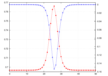
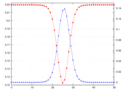
Figure 2: Left figure: particle soliton in region I₊. Right figure: hole soliton in region II₊. Red line shows magnetization (density) $\cos\theta_{i}$. Blue line shows superfluid velocity $\varphi_{i+1}-\varphi_{i}$. Results obtained from numerical solutions of lattice equations (2). Transverse modulation was not included.

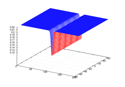
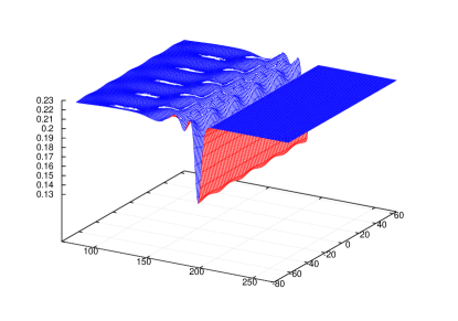
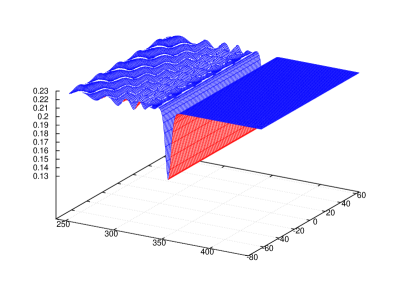
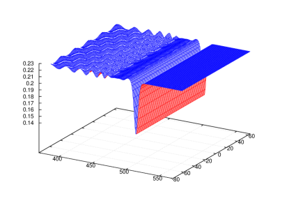
Figure 3: Time evolution of a soliton for $J_{z}/J_{\perp}=0$ in region II₊ in a 2d system. Horizontal axis are spatial coordinates. Vertical axis is magnetization (density). Different plots correspond to $tJ_{\perp}=0$, $10$, $30$, $50$. This soliton is stable to to small transverse modulation introduced explicitly in the initial state.

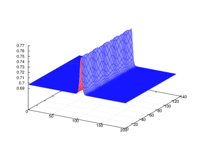
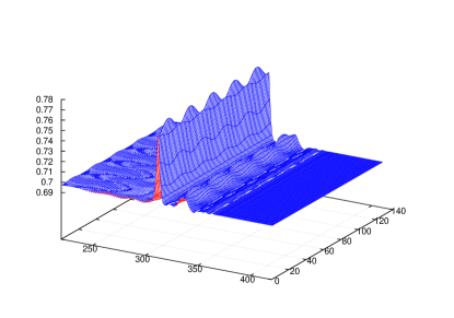
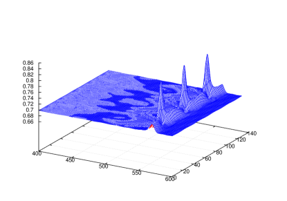
Figure 4: Time evolution of a soliton for $J_{z}/J_{\perp}=0$ in region I₊ in a 2d system. Axis are the same as in fig. 3 Different plots correspond to $tJ_{\perp}=0$, $40$, $80$, $90$. This soliton is unstable to small transverse modulation introduced explicitly in the initial state.

Parabolic and elliptic regimes. A rapidly growing oscillation zone characterizes elliptic instability for system (2) in region III on the phase diagram. It is shown in fig. 5. In supplementary material we show solution of (2) in the parabolic regime separating the elliptic and hyperbolic regions on the phase diagram 1.

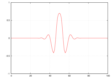
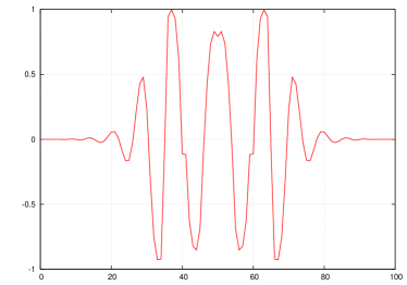
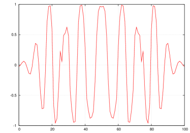
Figure 5: Time evolution of a small density perturbation in the elliptic region. Vertical axis is magnetization (density). Note rapidly developing oscillation zone typical to modulation instability. Different plots correspond to $tJ_{\perp}=0$, $2$, $4$, $6$.

Decay of magnetization step. We now discuss the problem of the decay of magnetization step in a system of type (1). Configurations of this type have been recently realized in 3d magnetic systems using tunable magnetic field gradientMedley2011 . They can be created for strongly correlated spinless bosons in 2d optical lattices using local addressability Bakr2010a ; Sherson2010a . Besides this experimental motivation, relaxation of the magnetization (density) step is an important methodological problem. Dynamics starting from this state allows extended unattenuated propagation of the magnetization (density) modulation, which should amplify the role of nonlinearities. This may be contrasted to e.g. dynamics starting with a ring type inhomogeneity, where already at the level of linear hydrodynamics there is a decrease of the magnetization (density) modulation in time. In classical hydrodynamics decay of the density step is one of the canonical problems considered in Refs. Gurevich1973 ; Gurevich1974 ; Lax1979 .

Fig. 6 shows the main stages of the magnetization step decay in regions I_±, II_±, IV: separation of left- and right-moving parts, steepening of one of the moving edges and formation of the oscillatory front. While there is general agreement between small amplitude limit analyzed in ref. Demler2011a and results of numerical analysis of lattice equations presented in fig. 6, there is one important difference. In the oscillatory region appearing from the decay of a large amplitude magnetization step we observe pairing of solitons, which can be understood as a result of interaction between solitons through the background of small amplitude waves. This is manifestation of the absence of exact integrability of lattice equations (2).

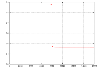
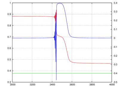
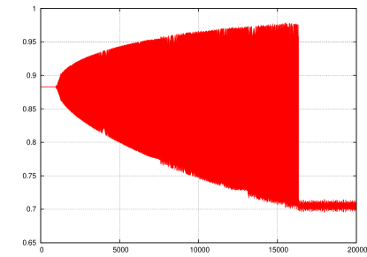
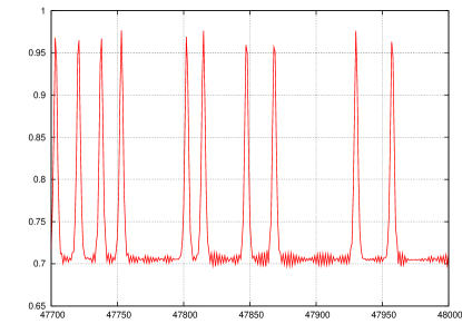
Figure 6: Decay of the density step in Region I₊. Red lines describe density, blue line corresponds to the phase difference. (a) Initial state $t=0$. (b) After $tJ_{\perp}=25$ of the evolution. Note separation of the right and left moving parts and formation of the oscillatory region on the left moving part. (c) Expanded view of the left front after $tJ_{\perp}=5000$ showing formation of the leading edge of the oscillation zone. (d) Left front after $tJ_{\perp}=15000$. Note soliton pairing mediated by background waves with small amplitude.

Experimental considerations. Direct experimental tests of theoretical results presented in this paper can be obtained by analyzing dynamics starting from soliton configurations of ultracold atoms in optical lattices, such as shown in figs 2, 3, 4. These figures show that lattices of the order of tens of sites should be sufficient for such studies. Experimentally soliton like initial states can be created and their dynamics can be studied using single site resolution and addressability available in current experiments with ultracold atoms in optical lattices. Density modulation can be achieved by letting the system reach equilibrium with a specified inhomogeneous potential. Phase modulation can be done by applying a short potential pulse. We note that clear signatures of soliton dynamics can be achieved by starting with initial states that have density modulation and no phase imprinting. In this case a pair of solitons appears and propagates in the opposite directions. This process takes place on relatively short time scales accessible to experiments. Additional details about this procedure are discussed in the supplementary material. We also note that to observe soliton dynamics one does not need to create initial configuration, which match theoretically calculated solitonic solutions exactly. Numerical analysis of (2) shows that initial conditions with spatially localized excess or deficit of magnetization (density) separate reasonably fast into solitons and the wave background. On the other hand observing all stages of the magnetization (density) step decay requires longer times and larger system sizes. Another important experimental consideration, which we did not address so far, is the presence of the parabolic confining potential in all of the currently available experimental set-ups. In fig 7 we show that as long as the chemical potential change is not taking the system across one of the boundaries in fig. 1, it has no strong effect on the soliton propagation. However crossing any of the boundaries leads to the soliton break-up.

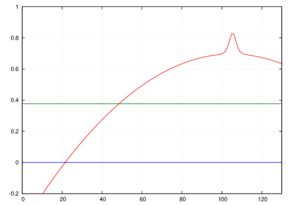
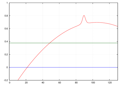
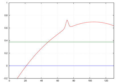
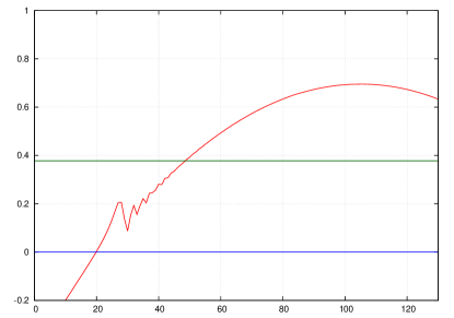
Figure 7: Soliton dynamics in the presence of parabolic potential. Soliton propagation is stable when parabolic potential is not taking the system across boundaries of different regions(figs a-c). Crossing the phase boundary causes the soliton break-up (fig d). Green line marks the boundary between regions I₊ and II₊.

Summary. We analyzed semiclassical dynamics of anisotropic Heisenberg models in dimension higher than one. Combining analytical study of small amplitude, long wavelength excitations with numerical studies of large amplitude, short wavelength excitations we demonstrated the existence of a universal dynamical phase diagram, in which different regions can be distinguished based on the character of one dimensional solitonic excitations, and stability of such solitons to transverse modulation. Universality of dynamics, which we find from direct solution of lattice equations, is very intriguing. Our model is not a special lattice regularization of an integrable continuum system. We analyze lattice model describing real physical systems which, in principle, can contain many terms breaking universality.

We thank I. Bloch, M. Greiner, M. Lewenstein, D. Pekker, and L. Pitaevskii for insightful discussions. This work was partially supported by the NSF Grant No. DMR-07-05472, DARPA OLE program, CUA, AFOSR Quantum Simulation MURI, AFOSR MURI on Ultracold Molecules, the ARO-MURI on Atomtronics (E.D.), Russian Federation Government Grant No. 2010-220-01-077, Grant RFBR No. 11-01-12067-ofi-m-2011 (A.M.). We also acknowledge support from the Harvard ITAMP and the Russian Quantum Center (RQC).

Supplementary material

Semiclassical dynamics. We consider time-dependent variational wavefunctions

$$|\Psi(t)\rangle=\prod_{i}\left[\sin{\theta_{i}(t)\over 2}\,e^{-i\varphi_{i}(t)\over 2}|\downarrow\rangle_{i}+\cos{\theta_{i}(t)\over 2}\,e^{i\varphi_{i}(t)\over 2}\,|\uparrow\rangle_{i}\right]$$ (3)

To project quantum dynamics into these wavefunctions we define the Lagrangian Jackiw1979 ; Huber2008 ; Demler2011a

$$\begin{array}[]{c}{\cal L}\,=\,-i\,\langle\Psi|\frac{d}{dt}|\Psi\rangle+\langle\Psi|H|\Psi\rangle\,\,=\cr\cr=\,\sum_{i}{1\over 2}\,{\dot{\varphi}}_{i}\,\cos\theta_{i}\,-\,J_{z}\,\sum_{i,j=i\pm 1}\cos\theta_{i}\,\cos\theta_{j}\,-\cr\cr-\,J_{\perp}\,\sum_{i,j=i\pm 1}\sin\theta_{i}\,\sin\theta_{j}\,\cos(\varphi_{i}-\varphi_{j})\end{array}$$ (4)

and write Lagrange equations for all variables. We obtain

$$\begin{array}[]{c}{\dot{\varphi}}_{i}\sin\theta_{i}=4J_{z}\sin\theta_{i}\left(\cos\theta_{i+1}+\cos\theta_{i-1}\right)-\cr-4J_{\perp}\cos\theta_{i}\left(\sin\theta_{i+1}\cos(\varphi_{i}-\varphi_{i+1})+\sin\theta_{i-1}\cos(\varphi_{i}-\varphi_{i-1})\right)\cr\cr{\dot{\theta}}_{i}=-4J_{\perp}\left(\sin\theta_{i+1}\sin(\varphi_{i}-\varphi_{i+1})+\sin\theta_{i-1}\sin(\varphi_{i}-\varphi_{i-1})\right)\end{array}$$ (5)

Introducing variables $x_{i}$, $y_{i}$ and $z_{i}$ we obtain equations (2) of the main text.

Nonlinear Hydrodynamics. To describe the regime of long wavelength modulations we introduce slow variables in space and time $X=hx$, $T=ht$, where $h$ is the lattice constant. We also define $\mu=\cos\theta$ and $\sigma(X,T)=h\varphi(X,t)$. Taking $h$ to be a small parameter we obtain

$$\begin{array}[]{c}{\cal L}\,\,=\,\,{1\over 2}\,\sigma_{T}\,\mu\,-\,2\,J_{\perp}\,(1-\mu^{2})\,\cos\sigma_{X}\,-\,2\,J_{z}\,\mu^{2}\,+\cr\cr+\,h^{2}\,J_{\perp}\,(1-\mu^{2})\,\left({1\over 3}\,\sigma_{XXX}\,\sin\sigma_{X}\,+\,{1\over 4}\,\sigma_{XX}^{2}\,\cos\sigma_{X}\right)\,+\cr\cr+\,h^{2}\,J_{\perp}\,{\mu^{2}\mu_{X}^{2}\over 1-\mu^{2}}\,\cos\sigma_{X}\,-\,h^{2}\,J_{z}\,\mu\,\mu_{XX}\,\,+\,\,{\cal O}(h^{4})\end{array}$$ (6)

Linearizing equations of motion around a uniform state we have

$$r^{1,2}_{T}\,=\,\pm\,\lambda(r^{1},r^{2})\,r^{1,2}_{X}$$ (7)

with $\lambda\,=\,4\,\sqrt{2\,J_{\perp}\,(1-\mu^{2})\,(\,J_{\perp}\,-\,J_{z})}$. Here $r^{1,2}$ are Riemann invariants Demler2011a that have physical interpretation of left and right moving perturbations. When $\lambda$ is real we have hyperbolic regime of the system, when $\lambda$ is imaginary we have elliptic regime. Special lines $J_{z}/J_{\perp}=1$ and $\mu_{0}=\pm 1$ have $\lambda=0$ and correspond to the parabolic regime.

Relation to Korteweg de Vries equations and solitons. To understand the character of solitons in the hyperbolic regime we take equations of motion obtained from (6) and keep only the lowest order terms in nonlinearity. We further assume that left and right moving components of the perturbation can be considered separately (e.g. we assume that left/right moving parts separate spatially before effects of nonlinearity become important)

$$r^{1}_{T}\,\,=\,\,-\,6\,\mu_{0}\,\sqrt{J_{\perp}(J_{\perp}-J_{z})}\,\,r^{1}\,\,r^{1}_{X}\,+$$ (8)

$$+\,h^{2}\sqrt{{2J_{\perp}(1-\mu_{0}^{2})\over J_{\perp}-J_{z}}}\left(J_{\perp}\left({1\over 6}-{\mu_{0}^{2}\over 1-\mu_{0}^{2}}\right)-{7\over 6}J_{z}\right)r^{1}_{XXX}$$

$$r^{2}_{T}\,\,=\,\,6\,\mu_{0}\,\sqrt{J_{\perp}(J_{\perp}-J_{z})}\,\,r^{2}\,\,r^{2}_{X}\,-$$ (9)

$$-\,h^{2}\sqrt{{2J_{\perp}(1-\mu_{0}^{2})\over J_{\perp}-J_{z}}}\left(J_{\perp}\left({1\over 6}-{\mu_{0}^{2}\over 1-\mu_{0}^{2}}\right)-{7\over 6}J_{z}\right)r^{2}_{XXX}$$

Equations (8), (9) are of the KdV type except for special lines

$$\mu_{0}\,=\,0\,\,\,\,\,\,\,\,,\,\,\,\,\,\,\,\,J_{\perp}\,\left({1\over 6}\,-\,{\mu_{0}^{2}\over 1-\mu_{0}^{2}}\right)\,-\,{7\over 6}\,J_{z}\,\neq\,0$$ (10)

Analysis of solitons, including their stability to transverse modulation can now be performed as discussed in ref. Demler2011a . Equation (10) gives phase boundaries shown in fig. 1 of the main text.

Imperfect preparation of the initial state.

An important question for experimental realizations of solitons is dynamics from initial states that do not match exactly soliton solutions. Fig. 8 shows that in this case the system separates perturbations into solitons and wave-trains.

Parabolic regime.

In Fig. 9 we show dynamics of solutions in the parabolic regime separating the elliptic and hyperbolic regions of the phase diagram 1 in the main text.

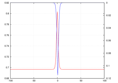
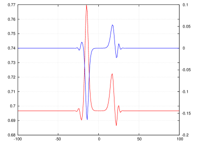
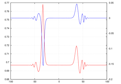
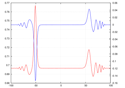
Figure 8: Dynamics from a general initial state, which does not match a solitonic solution. Red lines show magnetization (density), blue lines show superfluid velocity, $\phi_{i}-\phi_{i+1}$. Initial parameters correspond to region ${\rm I}_{+}$. Different plots are for $tJ_{\perp}=0$, $5$, $10$, $15$. Note separation of perturbations into solitons and wave-trains.

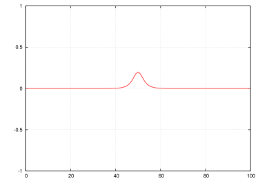
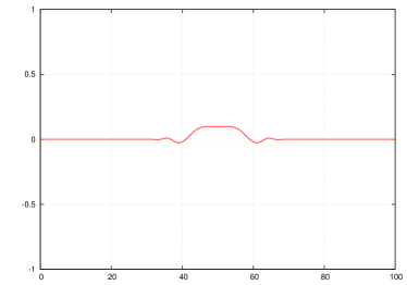
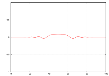
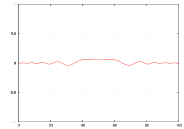
Figure 9: Time evolution of a small density perturbation on the parabolic line. Vertical axis is magnetization (density). Note a slowly growing oscillation region. Different plots correspond to $tJ_{\perp}=0$, $2$, $4$, $6$.

References

- (1) Stefano Giorgini and Sandro Stringari. Theory of ultracold atomic Fermi gases. Reviews of Modern Physics, 80(4):1215–1274, October 2008.
- (2) Franco Dalfovo, Stefano Giorgini, I Povo, Lev P Pitaevskii, and Sandro Stringari. Theory of Bose-Einstein condensation in trapped gases. Revews of Modern Physics, 71(3):463–512, 1999.
- (3) R. Shankar. Renormalization-group approach to interacting fermions. Revews of Modern Physics, 66(1):129, 1994.
- (4) S Nascimbène, N Navon, K J Jiang, F Chevy, and C Salomon. Exploring the thermodynamics of a universal Fermi gas. Nature, 463(7284):1057–60, February 2010.
- (5) M. Cross and P. Hohenberg. Pattern formation outside of equilibrium. Reviews of Modern Physics, 65(3):851–1112, July 1993.
- (6) Toshiya Kinoshita, Trevor Wenger, and David S Weiss. A quantum Newton’s cradle. Nature, 440(7086):900–3, April 2006.
- (7) Michael Moeckel and Stefan Kehrein. Interaction Quench in the Hubbard Model. Physical Review Letters, 100(17):1–4, May 2008.
- (8) Marcos Rigol, Vanja Dunjko, and Maxim Olshanii. Thermalization and its mechanism for generic isolated quantum systems. Nature, 452(7189):854–8, April 2008.
- (9) Peter Barmettler, Matthias Punk, Vladimir Gritsev, Eugene Demler, and Ehud Altman. Relaxation of Antiferromagnetic Order in Spin-1/2 Chains Following a Quantum Quench. Physical Review Letters, 102(13):1–4, April 2009.
- (10) Anatoli Polkovnikov, Krishnendu Sengupta, Alessandro Silva, and Mukund Vengalattore. Colloquium: Nonequilibrium dynamics of closed interacting quantum systems. Reviews of Modern Physics, 83(3):863–883, August 2011.
- (11) Ulrich Schneider, Lucia Hackerm, Jens Philipp Ronzheimer, Sebastian Will, Simon Braun, Thorsten Best, Immanuel Bloch, Eugene Demler, Stephan Mandt, David Rasch, and Achim Rosch. Breakdown of diffusion: From collisional hydrodynamics to a continuous quantum walk in a homogeneous Hubbard model. Nature Physics, 2012.
- (12) M Gring, M Kuhnert, T Langen, T Kitagawa, B Rauer, M Schreitl, I Mazets, D A Smith, E Demler, and J Schmiedmayer. Relaxation Dynamics and Pre-thermalization in an Isolated Quantum System. arXiv:1112.0013, pages 4–7, 2011.
- (13) Immanuel Bloch and Wilhelm Zwerger. Many-body physics with ultracold gases. Reviews of Modern Physics, 80(3):885–964, July 2008.
- (14) Maciej Lewenstein, Anna Sanpera, and Veronica Ahufinger. Advances in Physics Ultracold atomic gases in optical lattices : mimicking condensed matter physics and beyond. Advances in Physics, 56(December 2011):243–379, 2007.
- (15) Karl D. Nelson, Xiao Li, and David S. Weiss. Imaging single atoms in a three-dimensional array. Nature Physics, 3(8):556–560, June 2007.
- (16) Nathan Gemelke, Xibo Zhang, Chen-Lung Hung, and Cheng Chin. In situ observation of incompressible Mott-insulating domains in ultracold atomic gases. Nature, 460(7258):995–8, August 2009.
- (17) Jacob F Sherson, Christof Weitenberg, Manuel Endres, Marc Cheneau, Immanuel Bloch, and Stefan Kuhr. Single-atom-resolved fluorescence imaging of an atomic Mott insulator. Nature, 467(7311):68–72, September 2010.
- (18) W S Bakr, a Peng, M E Tai, R Ma, J Simon, J I Gillen, S Fölling, L Pollet, and M Greiner. Probing the superfluid-to-Mott insulator transition at the single-atom level. Science (New York, N.Y.), 329(5991):547–50, July 2010.
- (19) Austen Lamacraft and Joel Moore. Potential insights into non-equilibrium behavior from atomic physics. In Alexander Fetter, Katherine Levin, and Dan Stamper-Kurn, editors, Ultracold Bosonic and Fermionic Gases.
- (20) Immanuel Bloch. Collapse and revival of the matter wave field of a Bose – Einstein condensate. Nature, 419(September):3–6, 2002.
- (21) Niels Strohmaier, Daniel Greif, Robert Jördens, Leticia Tarruell, Henning Moritz, and Tilman Esslinger. Observation of Elastic Doublon Decay in the Fermi-Hubbard Model. Physical Review Letters, 104(8):1–4, February 2010.
- (22) Yu-Ao Chen, Sebastian D. Huber, Stefan Trotzky, Immanuel Bloch, and Ehud Altman. Many-body Landau–Zener dynamics in coupled one-dimensional Bose liquids. Nature Physics, 7(1):61–67, October 2010.
- (23) Marc Cheneau, Peter Barmettler, Dario Poletti, Manuel Endres, Peter Schauß, Takeshi Fukuhara, Christian Gross, Immanuel Bloch, Corinna Kollath, and Stefan Kuhr. Light-cone-like spreading of correlations in a quantum many-body system. arXIv:1111.0776, 2011.
- (24) L.-M. Duan, E. Demler, and M. Lukin. Controlling Spin Exchange Interactions of Ultracold Atoms in Optical Lattices. Physical Review Letters, 91(9):1–4, August 2003.
- (25) a. B. Kuklov and B. V. Svistunov. Counterflow Superfluidity of Two-Species Ultracold Atoms in a Commensurate Optical Lattice. Physical Review Letters, 90(10):12–15, March 2003.
- (26) Ehud Altman, Walter Hofstetter, Eugene Demler, and Mikhail D Lukin. Phase diagram of two-component bosons on an optical lattice. New Journal of Physics, 5:113–113, September 2003.
- (27) S Trotzky, P Cheinet, S Fölling, M Feld, U Schnorrberger, a M Rey, a Polkovnikov, E a Demler, M D Lukin, and I Bloch. Time-resolved observation and control of superexchange interactions with ultracold atoms in optical lattices. Science (New York, N.Y.), 319(5861):295–9, January 2008.
- (28) G Batrouni, R Scalettar, G Zimany, and A Kampf. Supersolids in the Bose-Hubbard Hamiltonian. Physical Review Letters, 74(13):2527–2530, 1995.
- (29) V. Scarola and S. Das Sarma. Quantum Phases of the Extended Bose-Hubbard Hamiltonian: Possibility of a Supersolid State of Cold Atoms in Optical Lattices. Physical Review Letters, 95(3):3–6, July 2005.
- (30) T Lahaye, C Menotti, L Santos, M Lewenstein, and T Pfau. The physics of dipolar bosonic quantum gases. Reports on Progress in Physics, 72(12):126401, December 2009.
- (31) Eugene Demler and Andrei Maltsev. Semiclassical solitons in strongly correlated systems of ultracold bosonic atoms in optical lattices. Annals of Physics, 326(7):1775–1805, July 2011.
- (32) Radha Balakrishnan, Indubala I. Satija, and Charles W. Clark. Particle-Hole Asymmetry and Brightening of Solitons in a Strongly Repulsive Bose-Einstein Condensate. Physical Review Letters, 103(23):1–4, December 2009.
- (33) S. Burger, K. Bongs, S. Dettmer, W. Ertmer, and K. Sengstock. Dark Solitons in Bose-Einstein Condensates. Physical Review Letters, 83(25):5198–5201, December 1999.
- (34) Magnus Johansson and Yuri Kivshar. Discreteness-Induced Oscillatory Instabilities of Dark Solitons. Physical Review Letters, 82(1):85–88, January 1999.
- (35) J. Denschlag. Generating Solitons by Phase Engineering of a Bose-Einstein Condensate. Science, 287(5450):97–101, January 2000.
- (36) Andrea Trombettoni and Augusto Smerzi. Discrete Solitons and Breathers with Dilute Bose-Einstein Condensates. Physical Review Letters, 86(11):2353–2356, March 2001.
- (37) Kevin E Strecker, Guthrie B Partridge, Andrew G Truscott, and Randall G Hulet. Formation and propagation of matter-wave soliton trains. Nature, 417(6885):150–3, May 2002.
- (38) L Khaykovich, F Schreck, G Ferrari, T Bourdel, J Cubizolles, L D Carr, Y Castin, and C Salomon. Formation of a matter-wave bright soliton. Science (New York, N.Y.), 296(5571):1290–3, May 2002.
- (39) B Baizakov, B Malomed, and M Salerno. Multidimensional solitons in periodic potentials. Europhysics letters, 63:642, 2003.
- (40) P. Kevrekidis, R. Carretero-González, G. Theocharis, D. Frantzeskakis, and B. Malomed. Stability of dark solitons in a Bose-Einstein condensate trapped in an optical lattice. Physical Review A, 68(3):2–5, September 2003.
- (41) V. Ahufinger, a. Sanpera, P. Pedri, L. Santos, and M. Lewenstein. Creation and mobility of discrete solitons in Bose-Einstein condensates. Physical Review A, 69(5):12–15, May 2004.
- (42) B. Eiermann, Th. Anker, M. Albiez, M. Taglieber, P. Treutlein, K.-P. Marzlin, and M. Oberthaler. Bright Bose-Einstein Gap Solitons of Atoms with Repulsive Interaction. Physical Review Letters, 92(23):1–4, June 2004.
- (43) Christoph Becker, Simon Stellmer, Parvis Soltan-Panahi, Sören Dörscher, Mathis Baumert, Eva-Maria Richter, Jochen Kronjäger, Kai Bongs, and Klaus Sengstock. Oscillations and interactions of dark and dark–bright solitons in Bose–Einstein condensates. Nature Physics, 4(6):496–501, May 2008.
- (44) R. Scott, F. Dalfovo, L. Pitaevskii, and S. Stringari. Dynamics of Dark Solitons in a Trapped Superfluid Fermi Gas. Physical Review Letters, 106(18):185301, May 2011.
- (45) a. Kamchatnov and L. Pitaevskii. Stabilization of Solitons Generated by a Supersonic Flow of Bose-Einstein Condensate Past an Obstacle. Physical Review Letters, 100(16):160402, April 2008.
- (46) Patrick Medley, David Weld, Hirokazu Miyake, David Pritchard, and Wolfgang Ketterle. Spin Gradient Demagnetization Cooling of Ultracold Atoms. Physical Review Letters, 106(19):1–4, May 2011.
- (47) A.V. Gurevich and L.P. Pitaevskii. Decay of initial discontinuity in the Kortweg - de Vries equation. JETP Letters, 17:193, 1973.
- (48) A V Gurevich and L P Pitaevskit. Nonstationary structure of a collision less shock wave. Sov. Phys. JETP, 38(3):291–297, 1974.
- (49) P D Lax and C D Levermore. The zero dispersion limit for the Korteweg-deVries KdV equation. Proceedings of the National Academy of Sciences of the United States of America, 76(8):3602–6, August 1979.
- (50) R Jackiw and A Kerman. Time-dependent variational principle and the effective action. Physics Letters, 71(2):1–5, 1979.
- (51) S. Huber, B. Theiler, E. Altman, and G. Blatter. Amplitude Mode in the Quantum Phase Model. Physical Review Letters, 100(5):50404, February 2008.