Stochastic Domination and Comb Percolation

Abstract.

There exists a Lipschitz embedding of a $d$-dimensional comb graph (consisting of infinitely many parallel copies of ${\mathbb{Z}}^{d-1}$ joined by a perpendicular copy) into the open set of site percolation on ${\mathbb{Z}}^{d}$, whenever the parameter $p$ is close enough to $1$ or the Lipschitz constant is sufficiently large. This is proved using several new results and techniques involving stochastic domination, in contexts that include a process of independent overlapping intervals on ${\mathbb{Z}}$, and first-passage percolation on general graphs.

1. Introduction

The following natural generalization of percolation theory is prompted by the results of [2, 7]. Let $G$ and $H$ be graphs. For $p\in[0,1]$, consider the site percolation model on $H$, in which each vertex is open with probability $p$, and otherwise closed, independently for different vertices. An embedding of $G$ in the open set of $H$ is an injective map from the vertex set of $G$ to the set of open vertices of $H$, such that neighbours in $G$ map to neighbours in $H$. Define the critical probability

$$p_{c}(G,H):=\\ \inf\Bigl{\{}p:{\mathbb{P}}\bigl{(}\exists\text{ an embedding of $G$ in the open set of $H$}\bigr{)}>0\Bigr{\}}.$$

If ${\mathbb{Z}}_{+}$ is a singly-infinite path then $p_{c}({\mathbb{Z}}_{+},H)$ is simply the usual critical probability $p_{c}(H)$ of site percolation on $H$ (see e.g. [5] for background). For the doubly-infinite path ${\mathbb{Z}}$, it was proved in [11, Proof of Theorem 3.9] that $p_{c}({\mathbb{Z}},H)$ also equals $p_{c}(H)$ for any infinite connected $H$. Observe that if $G,H$ are subgraphs of $G^{\prime},H^{\prime}$ respectively then $p_{c}(G,H^{\prime})\leq p_{c}(G^{\prime},H)$.

We focus on the question: for which graphs is it the case that $p_{c}(G,H)<1$? Let ${\mathbb{Z}}^{d}$ be the usual cubic lattice, with vertex set also denoted ${\mathbb{Z}}^{d}$, and with vertices $x,y$ joined by an edge whenever $\|x-y\|_{1}=1$. Also let ${\mathbb{Z}}^{d}_{[M]}$ denote the spread-out lattice, in which vertices $x,y\in{\mathbb{Z}}^{d}$ are joined whenever $0<\|x-y\|_{\infty}\leq M$. It was proved in [2] and [7] respectively that $p_{c}({\mathbb{Z}}^{d-1},{\mathbb{Z}}^{d}_{[2]})<1$, while on the other hand $p_{c}({\mathbb{Z}}^{d},{\mathbb{Z}}^{d}_{[M]})=1$ for all $M$.

An embedding of $G$ into ${\mathbb{Z}}^{d}_{[M]}$ may also be regarded as an $M$-Lipschitz embedding of $G$ into ${\mathbb{Z}}^{d}$. In that language, the results mentioned in the previous paragraph say that $M$-Lipschitz embeddings of ${\mathbb{Z}}^{d-1}$ into ${\mathbb{Z}}^{d}$ are possible whenever $p$ or $M$ is large enough, while Lipschitz embeddings of ${\mathbb{Z}}^{d}$ into ${\mathbb{Z}}^{d}$ are never possible for $p<1$.

In this article we address a case lying between the last two mentioned above. Define the $d$-dimensional comb graph $\mathbb{K}^{d}$ to have vertex set ${\mathbb{Z}}^{d}$, and edges $(z,z+e_{i})$ for every $z\in{\mathbb{Z}}^{d}$ and all $i$ with $1\leq i\leq d-1$, together with $(z,z+e_{d})$ for all $z$ such that $z_{1}=0$ (where $e_{1},\dots,e_{d}$ are the standard basis vectors). Thus, $\mathbb{K}^{d}$ consists of a stack of parallel copies of ${\mathbb{Z}}^{d-1}$ (perpendicular to coordinate $d$), connected by a single perpendicular copy of ${\mathbb{Z}}^{d-1}$ (perpendicular to coordinate $1$). For $d>2$, $\mathbb{K}^{d}$ is isomorphic to the product of the $2$-dimensional comb $\mathbb{K}^{2}$ with ${\mathbb{Z}}^{d-2}$. See Figure 1 for illustrations of $\mathbb{K}^{2}$ and $\mathbb{K}^{3}$.

Figure 1. Part of the comb graph $\mathbb{K}^{d}$ in dimension $d=2$ (left) and $d=3$ (right).

Theorem 1 (Comb percolation).

We have $p_{c}(\mathbb{K}^{d},{\mathbb{Z}}^{d}_{[2]})<1$ for all $d\geq 2$.

Corollary 2.

For all $d\geq 2$ we have $p_{c}(\mathbb{K}^{d},{\mathbb{Z}}^{d}_{[M]})\to 0$ as $M\to\infty$.

Our proof gives an explicit upper bound for $p_{c}(\mathbb{K}^{d},{\mathbb{Z}}^{d}_{[2]})$, but we have not attempted to optimize it. The spread-out lattice ${\mathbb{Z}}^{d}_{[2]}$ in Theorem 1 cannot be replaced with the nearest-neighbour lattice ${\mathbb{Z}}^{d}$. Indeed, it was proved in [7] that $p_{c}({\mathbb{Z}}^{2},{\mathbb{Z}}^{d})=1$ for all $d\geq 2$; since ${\mathbb{Z}}^{2}$ is a subgraph of $\mathbb{K}^{d}$ this implies $p_{c}(\mathbb{K}^{d},{\mathbb{Z}}^{d})=1$ for $d\geq 3$. It is also easy to see that $p_{c}(\mathbb{K}^{2},{\mathbb{Z}}^{2})=1$, since the backbone of $\mathbb{K}^{2}$ would have to be embedded as a straight line in ${\mathbb{Z}}^{2}$. On the other hand, our techniques may be adapted to prove $p_{c}(\mathbb{K}^{d},H)<1$ for some graphs $H$ with edge sets intermediate between those of ${\mathbb{Z}}^{d}$ and ${\mathbb{Z}}^{d}_{[2]}$ – in particular it seems plausible that this could be done for the “star lattice” ${\mathbb{Z}}^{d}_{[1]}$, but we have not pursued this. Such questions reflect details of the local lattice geometry, whereas the fact that $p_{c}(\mathbb{K}^{d},{\mathbb{Z}}^{d}_{[M]})<1$ for large enough $M$ (as implied by Theorem 1) is more fundamental.

Our proof of Theorem 1 will make use of several new results and techniques involving stochastic domination, which we believe are of independent interest and wider applicability. Stochastic domination by i.i.d. processes is a powerful technique for proving results of this kind, because it enables facts proved for the i.i.d. case to be transferred to other settings. One widely used tool is the result of [10] that a $k$-dependent Bernoulli process with sufficiently high marginals dominates any given i.i.d. product measure. However, the key process that we will need to control (of “bad points”) is not $k$-dependent, and in fact is not dominated by any product measure. Therefore the methods we use are of a different nature.

Background on stochastic domination may be found in [9, Ch. II, §2], for example. For our purposes, the following definition via coupling will suffice. Let $X$ and $Y$ be random variables taking values in the same partially ordered space. Then we say that $X$ stochastically dominates $Y$ if there exist $X^{\prime},Y^{\prime}$ on some probability space with $X^{\prime}$ and $X$ equal in law, $Y^{\prime}$ and $Y$ equal in law, and $X^{\prime}\geq Y^{\prime}$ almost surely. The underlying partial order will be inclusion (in the case of random sets) or pointwise ordering (for real functions).

Our first tool is a simple but useful stochastic domination result on overlapping intervals in a one-dimensional setting. For $c\in(0,1)$, say that a random variable $X$ has geometric distribution with parameter $c$, denoted ${\text{Geom}}(c)$, if ${\mathbb{P}}(X=r)=(1-c)c^{r}$ for $r=0,1,2,\dots$. (Note that the value $0$ is included, and that $c$ is the probability of a “failure” rather than a “success”). In the following, the interval $(a,b)$ is taken to be empty if $a=b$.

Theorem 3 (One-dimensional domination).

Let $(G_{n})_{n\in{\mathbb{Z}}}$ be i.i.d. ${\text{Geom}}(c)$ random variables. The random set ${\mathbb{Z}}\cap\bigcup_{n\in{\mathbb{Z}}}\bigl{(}n-G_{n},n+G_{n}\bigr{)}$ is stochastically dominated by the open set of i.i.d. site percolation on ${\mathbb{Z}}$ with parameter $\min(4\surd c,1)$.

Our second tool concerns first-passage percolation. As we explain in Section 2, it can be regarded as unifying and generalizing ideas in [1, 4, 6]. Let $V$ be a countable vertex set. For every pair of distinct vertices $x,y\in V$, the directed edge $e=(x,y)$ is assigned a random passage time $W(e)=W(x,y)$ taking values in $[0,\infty]$. The passage times of different edges are independent but not necessarily identically distributed. (We can model a process on a graph other than the complete graph by taking some passage times to be $\infty$ almost surely.) In addition, each vertex $x\in V$ has a deterministic source time $t(x)\in(-\infty,\infty]$ at which it is “switched on”. (For example, to model growth started at a single source $a$ we would take $t(a)=0$ and $t(x)=\infty$ for all other $x$.) The occupation time of $x\in V$ is the time it is first reached:

$$T(x):=\inf_{\begin{subarray}{c}y_{0},y_{1},\ldots,y_{m}:\\ y_{m}=x\end{subarray}}\biggl{\{}t(y_{0})+\sum_{k=1}^{m}W(y_{k-1},y_{k})\biggr{\}}.$$

We now consider a collection of countably many models on the same vertex set, indexed by $i\in\mathcal{I}$. Different models have identically distributed passage times, and are independent of each other, but may have different source times. Write $t_{i}(x)$ for the source time of $x$ in model $i$, and $T_{i}(x)$ for the occupation time of vertex $x$ in this model. Let

$${\widetilde{T}}(x):=\inf_{i}T_{i}(x).$$

Finally, consider another model with source times given by

$$t(x):=\inf_{i}t_{i}(x),\quad x\in V,$$

and with the same passage time distributions as the other models. Write $T(x)$ for the occupation time of $x$ in this model.

Theorem 4 (First-passage percolation domination).

Under the above assumptions, $({\widetilde{T}}(x))_{x\in V}$ is stochastically dominated by $(T(x))_{x\in V}$.

We prove Theorems 3 and 4 at the end of the article. In the next section we explain how these results are used in the proof of Theorem 1.

2. Outline of Proof

In this section we explain the main ideas behind the proof of Theorem 1. Our starting point is the following strengthening of a result of [2] (the latter has been applied in [3, 8], and extended in other directions in [6]). For $x=(x_{1},\ldots,x_{d-1})\in{\mathbb{Z}}^{d-1}$ and $z\in{\mathbb{Z}}$ we denote their concatenation thus: $(x,z):=(x_{1},\ldots,x_{d-1},z)\in{\mathbb{Z}}^{d}$. Vertices of ${\mathbb{Z}}^{d}$ will sometimes be called sites.

Theorem 5 (Stacked Lipschitz surfaces).

Consider site percolation on ${\mathbb{Z}}^{d}$ with $d\geq 2$. If the parameter $p$ is sufficiently close to $1$ then a.s. there exist (random) functions $L_{n}:{\mathbb{Z}}^{d-1}\to{\mathbb{Z}}$, indexed by $n\in{\mathbb{Z}}$, with the following properties.

(1a) The site $$(x,L_{n}(x))\in{\mathbb{Z}}^{d} x\in{\mathbb{Z}}^{d-1} n\in{\mathbb{Z}}$$ is open for all and .

(1b) For each $$n L_{n} 1$$, the function is -Lipschitz in the sense that

$$\hskip 56.9055pt|L_{n}(x)-L_{n}(x^{\prime})|\leq 1\text{ whenever }\|x-x^{\prime}\|_{\infty}=1.$$

(1c) $$L_{n}(x)>2n x n$$ for all and .

(1d) $$L_{n-1}(x)<L_{n}(x) x n$$ for all and .

For each $n$, the graph $\big{\{}(x,L_{n}(x)):x\in{\mathbb{Z}}^{d-1}\big{\}}$ of $L_{n}$ is a “Lipschitz surface”, and Theorem 5 asserts the existence of an ordered stack of disjoint open Lipschitz surfaces. See Figure 2. This strengthens the result of [2] that one such surface exists for $p$ sufficiently close to $1$. Our Lipschitz surfaces differ from those in [2, 6] in that we use the $\infty$-norm rather than the $1$-norm in (1b) – this is relatively unimportant, but will be convenient for our construction. The condition (1c) will be helpful in keeping track of the typical position of each surface.

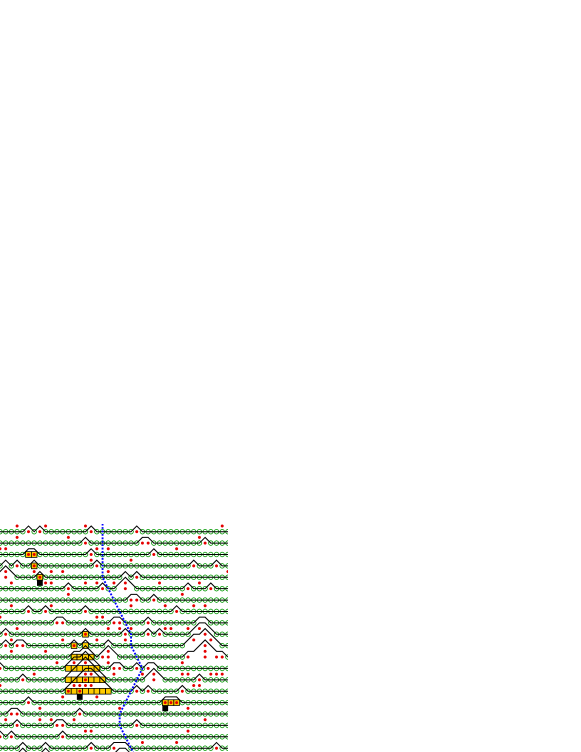
closed sites; stacked Lipschitz surfaces $L_{n}$ avoiding closed sites; good sites (where $L_{n}$ is as low as possible); perpendicular Lipschitz surface $H$ avoiding bad sites; three selected sites $y$; obstacles $A_{y}$ at those sites $y$.  

Figure 2. The main objects used in the construction of the embedding. Here $d=2$ and $p=0.885$.

In proving Theorem 5 we will define a particular family of functions $(L_{n})$ having additional desirable properties. In fact, $(L_{n})$ will be the minimal family satisfying (1a)–(1d) in the sense that for any other such family $(L_{n}^{\prime})$ we have $L_{n}(x)\leq L_{n}^{\prime}(x)$ for all $x,n$.

Our aim is to weave these Lipschitz surfaces together using another Lipschitz surface perpendicular to the stack. Observe that the minimum possible value of $L_{n}(x)$ is $2n+1$. We pay particular attention to those positions where this minimum is attained. Let ${\mathbb{Z}_{\text{\rm even}}}$ be the set of even integers and ${\mathbb{Z}_{\text{\rm odd}}}$ the set of odd integers. We call the site $(x,2n+1)\in{\mathbb{Z}}^{d-1}\times{\mathbb{Z}_{\text{\rm odd}}}$ good if $L_{n}(x)=2n+1$, and otherwise bad. Note that these definitions apply only to sites whose last coordinate is odd, and depend on the choice of the functions $L_{n}$. Since $(x,L_{n}(x))$ is always open, every good site is open.

Theorem 6 (Perpendicular Lipschitz surface).

Fix $d\geq 2$. For $p$ sufficiently close to $1$, the functions $L_{n}$ of Theorem  5 may be chosen so that almost surely there exists a function $H:{\mathbb{Z}}^{d-2}\times{\mathbb{Z}_{\text{\rm odd}}}\to{\mathbb{Z}}$ with the following properties.

(2a) $$\text{The site }(H(u),u)\text{ is good for all }u\in{\mathbb{Z}}^{d-2}\times{\mathbb{Z}_{\text{\rm odd}}}.$$

(2b) $$|H(u)-H(u^{\prime})|\leq 1\text{ whenever:}$$

$$\hskip 56.9055pt|u_{d-1}-u^{\prime}_{d-1}|\leq 2,\text{ and }|u_{i}-u^{\prime}_{i}|\leq 1\text{ for }i\leq d-2.$$

See Figure 2. The set $\{(H(u),u):{u\in{\mathbb{Z}}^{d-2}\times{\mathbb{Z}_{\text{\rm odd}}}}\}$ forms a kind of Lipschitz surface perpendicular to the $1$ coordinate direction. (The “${\leq}2$” in (2b) reflects the appearance of ${\mathbb{Z}_{\text{\rm odd}}}$ in the domain of $H$. Note that the $d-1$ coordinate of $u$ becomes the $d$ coordinate of $(H(u),u)$.) It is relatively straightforward to check that any functions $L_{n}$ and $H$ satisfying (1a)–(1d) and (2a)–(2b) give rise to an embedding of $\mathbb{K}^{d}$ in the open set of ${\mathbb{Z}}^{d}_{[2]}$, as required for Theorem 1. This is verified in Section 6; the function $H$ gives the backbone of the comb, while the $L_{n}$’s give the fins. Therefore our main task is to prove Theorems 5 and 6.

We will prove Theorem 5 via an extension of the methods of [2]: the Lipschitz surfaces will be constructed as duals to paths of a certain type, called $\Lambda$-paths. Now, since the property (2b) required for $H$ is essentially property (1b) of our Lipschitz function $L_{0}$ (modulo a change of coordinate system), an appealing idea is to try to deduce Theorem 6 from Theorem 5. The problem, of course, is that the process of good sites is not i.i.d. It is also not dominated by any i.i.d process (because a vertical column of $k$ consecutive closed sites gives rise to a bad set with volume of order $k^{d}$). Nonetheless, we will indeed deduce Theorem 6 from Theorem 5, using stochastic domination in more subtle ways.

We will proceed by re-expressing the process of bad sites. For each $y\in{\mathbb{Z}}^{d-1}\times{\mathbb{Z}_{\text{\rm even}}}$ we will define a random finite set $A_{y}$, called the obstacle at $y$, in such a way that

$$\{x:\text{$x$ is bad}\}=\bigcup_{y}A_{y}.$$

The field of obstacles will have the stationarity property that $(A_{y}+z)_{y}$ is equal in law to $(A_{y+z})_{y}$ for all $z$. The obstacle at $y$ will be the set of points that can be reached from $y$ by $\Lambda$-paths satisfying certain conditions.

The random sets $A_{y}$ will not be independent of each other (since the paths used in their construction are shared between different $y$’s). However, we will prove that they can be replaced with independent sets in the following sense. Let $(\widetilde{A}_{y})_{y}$ be mutually independent random sets, with $\widetilde{A}_{y}$ equal in law to $A_{y}$ for each $y$. We will show

(3) $$\bigcup_{y}A_{y}\text{ is stochastically dominated by }\bigcup_{y}\widetilde{A}_{y}.$$

A similar fact was proved in [6] in the context of a Lipschitz percolation model. An analogous property for a continuum percolation model was obtained in [1], and related ideas appeared earlier in [4]. We will prove (3) by expressing $A_{y}$ in terms of a first-passage percolation model (via the paths involved in its definition), and appealing to the much more general Theorem 4.

Our task is now reduced to proving the existence of a Lipschitz surface $H$ (as in (2b)) avoiding a collection of independent sets $\widetilde{A}_{y}$. The ideas behind the proof of Theorem 5 will easily show that the radius around $y$ of the random obstacle $A_{y}$ (and thus $\widetilde{A}_{y}$) has exponential tails for $p$ sufficiently close to $1$. However, for $d\geq 2$, this is not enough to allow domination of $\bigcup_{y}\widetilde{A}_{y}$ by an i.i.d. percolation process, since there the probability of a closed ball of radius $r$ decays exponentially in $r^{d}$.

The final ingredient is a deterministic observation which allows us to reduce to a one-dimensional process and hence overcome the above dimensionality problem. Here it is important that the object we seek is a Lipschitz surface. For $x\in{\mathbb{Z}}^{d}$ and $r>0$ define the ball $B(x,r):=\{z\in{\mathbb{Z}}^{d}:\|x-z\|_{\infty}<r\}$ and the one-dimensional stick $S(x,r):=\{x+ae_{d}:a\in{\mathbb{Z}}\text{ and }|a|<r\}$.

Lemma 7 (Balls and sticks).

Suppose $h:{\mathbb{Z}}^{d-1}\to{\mathbb{Z}}$ is $1$-Lipschitz (i.e. $|h(x)-h(x^{\prime})|\leq 1$ whenever $\|x-x^{\prime}\|_{\infty}\leq 1$). If the graph $\{(x,h(x)):x\in{\mathbb{Z}}^{d-1}\}$ does not intersect the stick $S(y,2r-1)$ then it does not intersect the ball $B(y,r)$.

Figure 3. A Lipschitz surface avoids a ball provided it avoids a stick.

See Figure 3 for an illustration. Using Lemma 7, it suffices to construct a Lipschitz surface that avoids a union of sticks $\bigcup_{x\in{\mathbb{Z}}^{d}}S(x,G_{x})$ with i.i.d geometric sizes $G_{x}$. This union consists of independent one-dimensional processes in each vertical line. Therefore we can use Theorem 3 to dominate it by an i.i.d. percolation process (with parameter that tends to $0$ as $p\to 1$), and deduce Theorem 6 from Theorem 5, and hence complete the proof of Theorem 1.

In the next four sections we carry out the steps outlined above to prove Theorem 1. The stacked surfaces $L_{n}$ are constructed in Section 3. Obstacles are defined and dominated by independent sets in Section 4, and their radii are bounded in Section 5. The remaining details (including the stick argument) are completed in Section 6. Finally we prove the general domination results, Theorems 3 and 4, in Sections 8 and 7 respectively. The first-passage percolation result is proved via dynamic coupling. For the one-dimensional domination result we employ a queueing interpretation.

3. Stacked Lipschitz surfaces

In this section we prove Theorem 5. We first construct the functions $L_{n}$, and then prove that they have the required properties. We sometimes refer to the positive and negative senses of the $d$ coordinate as up and down respectively, and the other coordinates as horizonal.

Define a $\Lambda$-path to be a sequence of sites $z(0),z(1),\dots,z(m)\in{\mathbb{Z}}^{d}$ such that for each $i<m$,

(4) $$z(i+1)-z(i)\in\{e_{d}\}\cup\Delta,$$

where

$$\Delta:=\biggl{\{}-e_{d}+\sum_{i=1}^{d-1}\alpha_{i}e_{i}:(\alpha_{1},\alpha_{2},\dots,\alpha_{d-1})\in\{-1,0,1\}^{d-1}\biggr{\}}.$$

That is, each step is up or down, but the down-steps may also be diagonal; there are $3^{d-1}$ different types of down-step since each of the first $d-1$ coordinates is allowed to remain the same or change by 1 in either direction. (Our definition of a $\Lambda$-path differs slightly from that in [2], where only $2d+1$ types of down-step were allowed. The difference reflects our use of the $\infty$-norm in (1b).) For an integer $r\geq 0$, we call a $\Lambda$-path $r$-open if its up-steps have distinct locations, and at most $r$ of them end with an open site, i.e. among the indices $i<m$ for which $z(i+1)-z(i)=e_{d}$, the sites $z(i+1)$ are all distinct, and at most $r$ of them are open. We write $y\stackrel{{\scriptstyle r}}{{\to}}z$ if there is an $r$-open $\Lambda$-path from $y$ to $z$.

Now define the random set of sites $S_{n}$ by

(5) $$S_{n}:=\bigl{\{}z:y\stackrel{{\scriptstyle r}}{{\to}}z\text{ for some }r\text{ and some }y\text{ with }y_{d}=2(n-r)\bigr{\}}.$$

Then let $L_{n}$ be the function whose graph lies just above $S_{n}$:

(6) $$L_{n}(x):=\min\bigl{\{}\ell\in{\mathbb{Z}}:(x,\ell)\not\in S_{n}\bigr{\}},$$

(where $\min\emptyset:=\infty$).

Proposition 8.

Let the functions $L_{n}$ be defined as above. If $p$ is sufficiently close to $1$, then a.s. $L_{n}(x)<\infty$ for all $n$ and $x$, and the properties (1a)–(1d) in Theorem 5 all hold.

Proof.

From the definition and the underlying stationarity of the percolation process, the process $(L_{n}(x))_{n,x}$ is stationary in the sense that $(L_{n+k}(x+y)-2k)_{n,x}$ has the same law for any $k\in{\mathbb{Z}}$ and $y\in{\mathbb{Z}}^{d-1}$. Hence for the first claim it is enough to show that $L_{0}(0)<\infty$ a.s.

In fact we will show that $L_{0}(0)$ has exponential tails. For $h>0$, we have ${\mathbb{P}}(L_{0}(0)>h)={\mathbb{P}}((0,h)\in S_{0})$, and this is at most the expected number of $r$-open $\Lambda$-paths from the hyperplane ${\mathbb{Z}}^{d-1}\times\{-2r\}$ to $(0,h)$, summed over all $r$. For such a path, let $C$ be the number of up-steps that end in a closed site, let $U$ be the number of up-steps that end in an open site, and let $D$ be the number of down-steps (including diagonal steps). Since the path is from ${\mathbb{Z}}^{d-1}\times\{-2r\}$ to $(0,h)$ we must have $C+U-D=h-(-2r)$, i.e. $U=D-C+h+2r$. Since the path is $r$-open we have $U\leq r$, or equivalently $A\geq 0$ where $A:=r-U$.

For given $U,C,D$, the number of ways to choose a $\Lambda$-path ending at $(0,h)$ together with an assignment of states open and closed to its up-steps is at most $K^{U+C+D}$, where $K:=3^{d-1}+2$. (There are $3^{d-1}$ possible directions for a down-step, and two possible states for an up-step). For any such choice, the probability that the chosen states match the percolation configuration is $p^{U}q^{C}\leq q^{C}$, where $q:=1-p$.

Therefore

$${\mathbb{P}}(L_{0}(0)>h) \leq\sum_{\begin{subarray}{c}U,C,D,r\geq 0:\\ C+U-D=h+2r,\\ U\geq r\end{subarray}}K^{U+C+D}q^{C}$$

$$\leq\sum_{A,D,r\geq 0}K^{2D+h+2r}q^{D+h+r+A}$$

$$=\big{(}Kq\big{)}^{h}\sum_{A\geq 0}q^{A}\sum_{D\geq 0}\big{(}K^{2}q\big{)}^{D}\sum_{r\geq 0}\big{(}K^{2}q\big{)}^{r},$$

which converges (exponentially fast) to $0$ as $h\to\infty$ whenever $q<K^{-2}$. (For the second inequality above, we rewrote $U$ and $C$ in terms of $A$ and dropped the conditions $U\geq 0$ and $C\geq 0$.)

Now we verify properties (1a)–(1d). For (1a), observe that, for some $y,r$ as in the definition of $S_{n}$, there is an $r$-open path to the site $(x,L_{n}(x)-1)$, but there is none to the site $(x,L_{n}(x))$. Thus the site $(x,L_{n}(x))$ must be open – if it were closed, the $r$-open path to $(x,L_{n}(x)-1)$ could be extended one step upward (or else it already passed through that site).

Next, note that from the definition of $S_{n}$, if $z\in S_{n}$ then $z+v\in S_{n}$ for all $v\in\Delta$. This gives the Lipschitz property for $L_{n}$ as required for (1b). For (1c) note that certainly $(x,2n)\in S_{n}$ for all $x$ and $n$. Finally, if $z\in S_{n}$ then $z+e_{d}\in S_{n+1}$, giving (1d). ∎

Proof of Theorem 5.

This is immediate from Proposition 8 above. ∎

4. Obstacles

In this section we define obstacles, and show that they can be dominated by independent versions. Let the functions $L_{n}$ be defined as in (6). As mentioned earlier, we say that

$$\text{site }(x,2n+1)\in{\mathbb{Z}}^{d-1}\times{\mathbb{Z}_{\text{\rm odd}}}\text{ is {good} if }L_{n}(x)=2n+1,$$

and otherwise it is bad. For $y\in{\mathbb{Z}}^{d-1}\times{\mathbb{Z}_{\text{\rm even}}}$ we define the obstacle at $y$ to be

(7) $$A_{y}:=\Bigl{\{}z\in{\mathbb{Z}}^{d-1}\times{\mathbb{Z}_{\text{\rm odd}}}:y\xrightarrow{\frac{z_{d}-y_{d}-1}{2}}z\Bigr{\}}.$$

Note that $A_{y}$ is defined only for $y$ of even height, while it consists of a set of sites of odd heights.

Lemma 9.

We have

$$\Bigl{\{}x\in{\mathbb{Z}}^{d-1}\times{\mathbb{Z}_{\text{\rm odd}}}:x\text{\rm\ is bad}\Bigr{\}}=\bigcup_{y\in{\mathbb{Z}}^{d-1}\times{\mathbb{Z}_{\text{\rm even}}}}A_{y}.$$

Proof.

From (5),(6) it follows that $z=(x,2n+1)\in{\mathbb{Z}}^{d-1}\times{\mathbb{Z}_{\text{\rm odd}}}$ is bad if and only if $z\in S_{n}$, which in turn is equivalent to the existence of $y\in{\mathbb{Z}}^{d-1}\times{\mathbb{Z}_{\text{\rm even}}}$ such that $y\xrightarrow{(z_{d}-y_{d}-1)/2}z.$ ∎

Now let $({\widetilde{A}}_{y})_{y\in{\mathbb{Z}}^{d-1}\times{\mathbb{Z}_{\text{\rm even}}}}$ be mutually independent random sets, with ${\widetilde{A}}_{y}$ equal in law to $A_{y}$ for each $y$.

Proposition 10.

With the above definitions, $\bigcup_{y}A_{y}$ is stochastically dominated by $\bigcup_{y}{\widetilde{A}}_{y}$.

Proof.

We rephrase the definition of obstacles in terms of a first-passage percolation model. Let each upward directed edge $(z,z+e_{d})$, $z\in{\mathbb{Z}}^{d}$ have passage time $1$ if $z+e_{d}$ is open, and 0 if $z+e_{d}$ is closed. Each downward directed edge $(z,z+v)$, $v\in\Delta$ has passage time $0$. All other edges have passage time $\infty$. Note that all the passage times are independent. We assign source time $t(y)=y_{d}/2$ to each site $y\in{\mathbb{Z}}^{d-1}\times{\mathbb{Z}_{\text{\rm even}}}$, and source time $\infty$ to all sites in ${\mathbb{Z}}^{d-1}\times{\mathbb{Z}_{\text{\rm odd}}}$. From the definition of $r$-open paths, for $z\in{\mathbb{Z}}^{d-1}\times{\mathbb{Z}_{\text{\rm odd}}}$, we have

(8) $$z\in\bigcup_{y}A_{y}\iff T(z)\leq\frac{z_{d}-1}{2}.$$

Now consider a countable family of models indexed by $y\in{\mathbb{Z}}^{d-1}\times{\mathbb{Z}_{\text{\rm even}}}$. All models have the same distribution of passage times as described above, and are independent of each other, but in model $y$, the only source is $y$, with $t(y)=y_{d}/2$ (all other sites have source time $\infty$). Write $T_{y}(z)$ for the passage time to $z$ in model $y$. The set of sites $z\in{\mathbb{Z}}^{d-1}\times{\mathbb{Z}_{\text{\rm odd}}}$ with $T_{y}(z)\leq(z_{d}-1)/2$ has the same law as $A_{y}$; let us define it to be ${\widetilde{A}}_{y}$. Thus the family $({\widetilde{A}}_{y})$ has precisely the distribution required. Writing ${\widetilde{T}}(z):=\inf_{y}T_{y}(z)$ and using (8), we have

(9) $$z\in\bigcup_{y}{\widetilde{A}}_{y}\iff{\widetilde{T}}(z)\leq\frac{z_{d}-1}{2}.$$

Theorem 4 tells us that $({\widetilde{T}}(z))$ is stochastically dominated by $(T(z))$. Using (8) and (9), this implies that $\bigcup_{y}A_{y}$ is stochastically dominated by $\bigcup_{y}{\widetilde{A}}_{y}$, as required. ∎

5. Radii of obstacles

Let $R_{y}$ be the radius of the obstacle at $y$, by which we mean the smallest $r$ such that $A_{y}\subseteq B(y,r)$ (recall that $B(y,r):=\{z\in{\mathbb{Z}}^{d}:\|y-z\|_{\infty}<r\}$). So $R_{y}=0$ if and only if $R_{y}$ is empty. Since all sites in $A_{y}$ must have $d$ coordinate strictly greater than $y_{d}$, we observe that $R_{y}$ is never equal to $1$, and also that $A_{y}\subseteq B(y+e_{d},R_{y})$. Recall that our geometric random variables are supported on the non-negative integers.

Lemma 11.

If $p$ is sufficiently close to $1$ then for each $y\in{\mathbb{Z}}^{d-1}\times{\mathbb{Z}_{\text{\rm even}}}$, the radius $R_{y}$ of the obstacle at $y$ is stochastically dominated by a ${\text{Geom}}(c)$ random variable, where $c=c(p)\to 0$ as $p\to 1$.

Proof.

Since as observed above, $R_{y}$ never takes the value $1$, it will be enough to show that ${\mathbb{P}}(R_{y}>r)<c^{r+1}$ for all $r\geq 1$. We use a path-counting argument similar to that already used in the proof of Proposition 8.

Suppose that $R_{y}>r$. Then by the definition of $A_{y}$ there exists $z$ with $\|y-z\|_{\infty}\geq r$ and $y\xrightarrow{(z_{d}-y_{d}-1)/2}z$. Consider some $(z_{d}-y_{d}-1)/2$-open $\Lambda$-path from $y$ to such a $z$, and as before let it have $U$ up-steps ending in open sites, $C$ up-steps ending in closed sites, and $D$ (diagonal- or) down-steps. Since the path is $(z_{d}-y_{d}-1)/2$-open we have

$$U\leq(z_{d}-y_{d}-1)/2=(U+C-D-1)/2,$$

and so $C-U-D-1\geq 0$. Since $\|y-z\|_{\infty}\geq r$, either $z_{d}-y_{d}\geq r$, in which case $U+C-D\geq r$, or else $z$ and $y$ differ by at least $r$ in some other coordinate, in which case $D\geq r$ (since only down-steps permit horizontal movement). Using the earlier inequality, in either case we have $U+C-r\geq 0$.

As before, let $K:=3^{d-1}+2$ and $q:=1-p$. Then, bounding via the expected number of paths,

$${\mathbb{P}}(R_{y}>r) \leq\sum_{\begin{subarray}{c}U,C,D\geq 0:\\ C-U-D-1\geq 0\\ U+C-r\geq 0\end{subarray}}K^{U+C+D}q^{C}$$

$$\leq\sum_{X,Y,D\geq 0}K^{Y+D+r}q^{(X+Y+D+r+1)/2}$$

$$=(K\surd q)^{r}\surd q\sum_{X\geq 0}\surd q^{X}\sum_{Y\geq 0}(K\surd q)^{Y}\sum_{D\geq 0}(K\surd q)^{D},$$

where in the second inequality we wrote $X:=C-U-D-1$ and $Y:=U+C-r$ and dropped the conditions $U,C\geq 0$. The last expression equals

$$\frac{\surd q}{(1-\surd q)(1-K\surd q)^{2}}\;(K\surd q)^{r}=Aa^{r},\text{say,}$$

(where $A=A(K,q)$ and $a=a(K,q)$ are defined by the last equality), provided $a<1$. Finally, we have $Aa^{r}\leq\max(A,a)^{r+1}$, and $\max(A,a)\to 0$ as $q\to 0$. ∎

6. Completing the embedding

In this section we conclude the proof of Theorem 1 by combining the various ingredients together with some geometric arguments. We start by proving Lemma 7, which states that balls may be replaced with sticks for the purposes of finding a Lipschitz function that avoids them.

Proof of Lemma 7.

For $z\in{\mathbb{Z}}^{d}$ we write $\widehat{z}:=(z_{1},\ldots,z_{d-1})$, so $z=(\widehat{z},z_{d})$. Let $r\geq 1$ (otherwise the ball and stick in the lemma are both empty). Suppose that $\{(x,h(x)):x\in{\mathbb{Z}}^{d-1}\}$ does intersect $B(y,r)$, say at the site $u=(\widehat{u},h(\widehat{u}))\in B(y,r)$. Thus $\|\widehat{u}-\widehat{y}\|_{\infty}\leq r-1$ and $|h(\widehat{u})-y_{d}|\leq r-1$. By the Lipschitz property, the former implies $|h(\widehat{u})-h(\widehat{y})|\leq r-1$. Therefore $|h(\widehat{y})-y_{d}|\leq 2r-2$. Thus $(\widehat{y},h(\widehat{y}))\in S(y,2r-1)$, and $\{(x,h(x)):x\in{\mathbb{Z}}^{d-1}\}$ intersects $S(y,2r-1)$. ∎

Next we check that the Lipschitz surfaces of Theorems 5 and 6 can be combined to give an embedding of the comb. A slightly subtle point in dimensions $d\geq 3$ is that the backbone surface $H$ will not typically “line up” with the stacked surfaces $L_{n}$ with respect to the intermediate coordinates $2,\ldots,d-1$. Nevertheless, the use of the $\infty$-norm in the definitions of ${\mathbb{Z}}^{d}_{[2]}$ gives enough wiggle room to permit an embedding. Suppose we are given the functions $L_{n}$ and $H$. For $z\in{\mathbb{Z}}^{d}$, define $x(z)\in{\mathbb{Z}}^{d-1}$ and $f(z)\in{\mathbb{Z}}^{d}$ by

(10) $$x(z):=\Bigl{(}z_{1}+H\bigl{(}(z_{2},z_{3},\ldots,z_{d-1},2z_{d}+1)\bigr{)},z_{2},\ldots,z_{d-1}\Bigr{)};$$

(11) $$f(z):=\Bigl{(}x(z),L_{2z_{d}+1}\big{(}x(z)\big{)}\Bigr{)}.$$

Lemma 12.

Suppose that the functions $L_{n}$ and $H$ satisfy the conditions of Theorems 5 and 6. Then the function $f$ defined above is an embedding of the comb $\mathbb{K}^{d}$ in the open set of ${\mathbb{Z}}^{d}_{[2]}$.

Proof of Lemma 12.

First observe that the site $f(z)$ is open for all $z$; this is immediate from (11) and property (1a) of $L_{n}$.

We next check that $f$ is injective. From (1d), the sites $(x,L_{n}(x))$ and $(x^{\prime},L_{n^{\prime}}(x^{\prime}))$ are distinct whenever $x\neq x^{\prime}$ or $n\neq n^{\prime}$. Suppose $z\neq z^{\prime}$. If $z$ and $z^{\prime}$ differ in any of the first $d-1$ coordinates then by (10), $x(z)\neq x^{\prime}(z)$, while if they differ in the $d$ coordinate then $2z_{d}+1\neq 2z^{\prime}_{d}+1$. Thus (11) gives $f(z)\neq f(z^{\prime})$, as required.

To show that $f$ is an embedding of the comb it remains to check that

(12) $$\|f(z)-f(z+e_{i})\|_{\infty}\leq 2$$

for all $z\in{\mathbb{Z}}^{d}$ and $i\leq d-1$, and also for $i=d$ whenever $z_{1}=0$. We first note the following key point. If $z_{1}=0$, then

(13) $$f(z)=\bigl{(}x(z),2z_{d}+1\bigr{)}.$$

This is because, by (2a), for $u=(z_{2},z_{3},\dots,z_{d-1},2z_{d}+1)$, the site $\big{(}H(u),u\big{)}$ is good, which means that

$$L_{2z_{d}+1}(x(z)) =L_{2z_{d}+1}(H(u),z_{2},z_{3},\dots,z_{d-1})$$

$$=2z_{d}+1,$$

so that the two expressions in (11) and (13) are the same.

We now verify that (12) holds in the cases claimed. First suppose that $z$ and $z^{\prime}$ differ by $1$ in the $i$th coordinate, where $i\leq d-1$, and that all the other coordinates agree. By the Lipschitz property (2b) of $H$, the first coordinates of $x(z)$ and $x(z^{\prime})$ differ by at most $1$, and clearly the same is true of the other coordinates. Hence by property (1b), we have $|L_{2z_{d}+1}(x(z))-L_{2z_{d}+1}(x(z^{\prime}))|\leq 1$. It follows that $\|f(z)-f(z^{\prime})\|_{\infty}\leq 1<2$.

Now suppose that $z$ and $z^{\prime}$ differ by $1$ in the last coordinate, and all the other coordinates agree, and suppose in addition that $z_{1}=0$. Thus $2z_{d}+1$ and $2z^{\prime}_{d}+1$ differ by $2$, and by (13), $f(z)=(x(z),2z_{d}+1)$ and $f(z^{\prime})=(x(z^{\prime}),2z^{\prime}_{d}+1)$. By (2b) and (10), the first coordinates of $x(z)$ and $x(z^{\prime})$ differ by at most $1$, and the other coordinates agree. Therefore $\|f(z)-f(z^{\prime})\|_{\infty}=2$ as required. ∎

We are ready to prove Theorem 6 and deduce Theorem 1.

Proof of Theorem 6.

We need to show that if $p$ is sufficiently close to $1$ there exists $H$ satisfying (2a) and (2b).

Condition (2a) says that the surface $\{(H(u),u)\}$ must avoid every obstacle $A_{y}$, and by Proposition 10, for this it suffices to instead find a surface avoiding the independent obstacles ${\widetilde{A}}_{y}$. As remarked in Section 5 we have $A_{y}\subseteq B(y+e_{d},R_{y})$ (and $y+e_{d}\in{\mathbb{Z}}^{d-1}\times{\mathbb{Z}_{\text{\rm odd}}}$), and by Lemma 11, $R_{y}$ is dominated by a geometric random variable whose parameter $c=c(p)$ can be made as small as desired by taking $p$ large enough. Therefore it remains to show that for $c$ sufficiently small there exists $H$ satisfying (2b) such that $\{(H(u),u):u\in{\mathbb{Z}}^{d-2}\times{\mathbb{Z}_{\text{\rm odd}}}\}$ avoids $\bigcup_{y\in{\mathbb{Z}}^{d-1}\times{\mathbb{Z}_{\text{\rm odd}}}}B(y,G_{y})$, where $(G_{y})$ are i.i.d. ${\text{Geom}}(c)$. Note that now all the relevant sites have odd heights.

Now we map ${\mathbb{Z}}^{d-1}\times{\mathbb{Z}_{\text{\rm odd}}}$ to ${\mathbb{Z}}^{d}$ via the transformation $(m,v,2n+1)\mapsto(v,n,m)$, for $v\in{\mathbb{Z}}^{d-2}$ and $m,n\in{\mathbb{Z}}$. It thus suffices to find a function $h:{\mathbb{Z}}^{d-1}\to{\mathbb{Z}}$ satisfying the same $1$-Lipschitz condition (1b) as $L_{0}$, and whose graph $\{(x,h(x)):x\in{\mathbb{Z}}^{d-1}\}$ avoids $\bigcup_{y\in{\mathbb{Z}}^{d}}B(y,G_{y})$ for $(G_{y})$ i.i.d. ${\text{Geom}}(c)$. (The transformation does not increase $\infty$-norms).

Now we apply Lemma 7. The graph of $h$ will avoid the balls $B(y,G_{y})$ provided it avoids the sticks $S(y,(2G_{y}-1)_{+})$. Observe also that if $G$ is ${\text{Geom}}(c)$ then $(2G-1)_{+}$ is dominated by a ${\text{Geom}}(c^{\prime})$ random variable, where $c^{\prime}=\surd c$, so it suffices to avoid $\mathcal{S}:=\bigcup_{y\in{\mathbb{Z}}^{d}}S(y,G_{y}^{\prime})$ where $(G_{y}^{\prime})$ are i.i.d. ${\text{Geom}}(c^{\prime})$.

The random set $\mathcal{S}$ consists of independent components in each of the lines $\{x\}\times{\mathbb{Z}}$, for $x\in{\mathbb{Z}}^{d-1}$. Within any such line, Theorem 3 shows that it is stochastically dominated by the open set of an i.i.d. percolation process with parameter $c^{\prime\prime}=4\surd c^{\prime}$. Thus the whole set $\mathcal{S}$ is dominated by the open set of an i.i.d. percolation process with parameter $c^{\prime\prime}$ on ${\mathbb{Z}}^{d}$. Hence it follows from Theorem 5 (exchanging the roles of open and closed sites) that there exists a function $h$ satisfying our requirements if $c^{\prime\prime}$ is sufficiently small. Since $c^{\prime\prime}=4\,c(p)^{1/4}$, this holds provided $p$ is sufficiently close to $1$. ∎

Proof of Theorem 1.

This is immediate from Lemma 12 and Theorems 5 and 6. ∎

Proof of Corollary 2.

Fix $k\geq 1$ and call the site $x\in{\mathbb{Z}}^{d}$ occupied if the cube $kx+[0,k)^{d}$ contains some open site in the percolation model. For any graph $G$, if there exists an embedding of $G$ in the occupied sites of ${\mathbb{Z}}_{[m]}^{d}$ then there exists an embedding of $G$ in the open sites of ${\mathbb{Z}}_{[km+k-1]}^{d}$: we simply choose one open site from the cube of each occupied site in the image. Therefore,

$$\Bigl{[}1-p_{c}(G,{\mathbb{Z}}_{[km+k-1]}^{d})\Bigr{]}^{k^{d}}\geq 1-p_{c}(G,{\mathbb{Z}}_{[m]}^{d}).$$

Setting $m=2$ and $G=\mathbb{K}^{d}$, and using the fact that $p_{c}(G,{\mathbb{Z}}_{[M]}^{d})$ is decreasing in $M$, the result follows from Theorem 1. ∎

7. First-passage percolation domination

In this section we prove Theorem 4. Recall that we have a collection of models indexed by $i$, and an additional model whose source times are given by infima of source times of the others. Write $W_{i}(e)$ and $W(e)$ for the passage time of edge $e$ in model $i$ and in the additional model respectively.

Proof of Theorem 4.

The argument is most straightforward in the case where the vertex set $V$ and the index set $\mathcal{I}$ are finite, and where a.s. the occupation times $T_{i}(x)$ are finite and distinct for all $i$ and $x$. (This property holds, for example, when all the source times are distinct and finite, and each edge passage time is either $\infty$ or some positive continuous random variable). We begin with this case, and then extend to the general case by a limiting argument.

We will define the collection of passage times $(W(e))$ as a function of the collection $(W_{i}(e))$, in such a way that $W(e)$ shares the common distribution of the $W_{i}(e)$, that the passage times $W(e)$ are independent for different $e$, and that ${\widetilde{T}}(x)\leq T(x)$ for all $x$. This explicit coupling implies the stochastic domination required. For a directed edge $(x,y)$ we set

$$W(x,y):=W_{i}(x,y),\text{ where $i$ minimizes }T_{i}(x).$$

First we aim to show that ${\widetilde{T}}(x)\leq T(x)$. We have

$$T(x)=\min_{\begin{subarray}{c}y_{0},y_{1},\dots,y_{m}\\ y_{m}=x\end{subarray}}\biggl{\{}t(y_{0})+\sum_{k=1}^{m}W(y_{k-1},y_{k})\biggr{\}}.$$

If $y_{0},y_{1},\dots,y_{m}$ is a minimizing path in the above expression, then for all $r$ with $0\leq r\leq m$,

$$T(y_{r})=t(y_{0})+\sum_{k=1}^{r}W(y_{k-1},y_{k}),$$

and in particular $T(y_{r})=T(y_{r-1})+W(y_{r-1},y_{r})$ for $1\leq r\leq m$.

We will show by induction that ${\widetilde{T}}(y_{r})\leq T(y_{r})$ for all such $r$. For the $r=0$ case, we have

$$T(y_{0})=t(y_{0})=\min_{i}t_{i}(y_{0})\geq\min_{i}T_{i}(y_{0})={\widetilde{T}}(y_{0}).$$

Now suppose ${\widetilde{T}}(y_{r-1})\leq T(y_{r-1})$. Let $i$ minimize $T_{i}(y_{r-1})$, so that $W(y_{r-1},y_{r})=W_{i}(y_{r-1},y_{r})$, and $T(y_{r})\geq{\widetilde{T}}(y_{r})=T_{i}(y_{r})$. Then

$$T(y_{r}) =T(y_{r-1})+W(y_{r-1},y_{r})$$

$$\geq T_{i}(y_{r-1})+W_{i}(y_{r-1},y_{r})$$

$$\geq T_{i}(y_{r})\geq{\widetilde{T}}(y_{r}),$$

completing the induction.

It remains to show that the $W(e)$ as defined are indeed independent with the required distributions. We will do this by giving a different construction of all the models. The idea is to run them simultaneously in real time, revealing the random passage times only when they are needed.

First consider a single model $i$. We begin by choosing all the passage times $W_{i}(e)$, with the correct distributions, but we do not yet reveal them. (We can think of them as written on cards associated with the edges, which will be turned over at the appropriate times). Label each vertex with a time by which it needs to be examined; initially these are just the source times. Now we repeatedly do the following. Find the vertex $x$ with the earliest (smallest) label among those that have not yet been examined. Then examine $x$, which is to say, reveal the passage times $W_{i}(x,y)$, $y\in V$ of all edges leading out of $x$, and relabel each vertex $y\neq x$ with the minimum of: its current label, and the label at $x$ plus $W_{i}(x,y)$. Repeat until all vertices have been examined. It is clear that the vertices are examined in order of their occupation times $T_{i}(x)$, and that when a vertex is examined it is labeled with its occupation time (and this label does not subsequently change). Our assumptions guarantee that these times are all distinct, and so the choice of which vertex to examine next is always unambiguous. (These claims may be checked formally by induction over the vertices in order of their occupation times).

Now consider simultaneously running all the models $i\in\mathcal{I}$ in the way just described. We first choose all the passage times independently, without revealing them. At each step we examine the unexamined vertex with the earliest label across all the models (and we examine it only in the minimizing model). Clearly each individual model evolves exactly as before (but with its steps interspersed with the others). Our assumptions guarantee that no two steps are simultaneous. Finally we construct the passage times $W(e)$ of the additional model: at each step, if the vertex that is examined (say vertex $x$ in model $i$) is the first to be examined among the copies of that vertex $x$ in all the models, then we in addition set $W(x,y)=W_{i}(x,y)$ for all $y\in V$. Since the label of vertex $x$ in model $i$ at this step is $\min_{i}T_{i}(x)$ ($={\widetilde{T}}(x)$), this agrees with the earlier definition of $W(x,y)$. The key point is that the decision to assign $W_{i}(x,y)$ to $W(x,y)$ is made before the value of $W_{i}(x,y)$ is revealed. It follows that the passage times $(W(e))$ assigned to the additional model are independent and have the correct distributions, as required.

To extend to the general case, we consider a sequence of approximating finite systems of the kind just considered. Without loss of generality, suppose that the index set $\mathcal{I}$ is contained in ${\mathbb{N}}$. In the $n$th system in our sequence of approximations, we take a finite vertex set $V^{(n)}$, such that $V^{(n)}\uparrow V$ as $n\to\infty$. All source times and passage times involving a vertex not in $V^{(n)}$ are set to infinity. Any source time for a vertex in $V^{(n)}$ that was previously be set to infinity is now instead given value $n$ (to ensure that every vertex in $V^{(n)}$ is reached in finite time). Furthermore we consider only models indexed by $i\in\{1,2,\dots,n\}$. Finally we perturb the source times of vertices in $V^{(n)}$, and the passage times of edges joining points of $V^{(n)}$, by adding an independent Uniform$(0,\tfrac{1}{n})$ random variable to each. (This means that the source times are no longer deterministic – however, we can regard the randomness as being on two levels: given any choices of the source times, we have a set of models with random passage times). This ensures that a.s., the finite system satisfies all of our earlier assumptions.

Write $T^{(n)}_{i}(x)$, ${\widetilde{T}}^{(n)}(x)$ and $T^{(n)}(x)$ for the passage times in the $n$th approximation. These quantities are finite for any $x\in V_{n}$. But also, since any set of vertices is eventually contained within $V_{n}$, and each model $i$ is eventually included in the system, it follows that for any finite set $A$, the random vectors $({\widetilde{T}}^{(n)}(x))_{x\in A}$ and $(T^{(n)}(x))_{x\in A}$ converge in distribution as $n\to\infty$ to $({\widetilde{T}}(x))_{x\in A}$ and $(T(x))_{x\in A}$ respectively. We know from the argument applied to the finite case that $({\widetilde{T}}^{(n)}(x))_{x\in A}$ is stochastically dominated by $(T^{(n)}(x))_{x\in A}$ for any $n$. Hence from the convergence in distribution as $n\to\infty$, we obtain also that in fact $({\widetilde{T}}(x))_{x\in A}$ is stochastically dominated by $(T(x))_{x\in A}$. Since this holds for any finite subset $A\subseteq V$, it follows that in fact $({\widetilde{T}}(x))_{x\in V}$ is stochastically dominated by $(T(x))_{x\in V}$, as desired. ∎

We remark that Theorem 4 may easily be extended for example to models with undirected edges instead of (or in addition to) directed edges, or with passage times at sites. As long as all the passage times are independent, exactly the same methods used above will continue to apply.

8. Domination in one dimension

In this section we prove Theorem 3. We start with the following one-sided version. The interval $[a,b)$ is taken to be empty if $a=b$.

Proposition 13.

For $c\in(0,1)$, let $(G_{n})_{n\in{\mathbb{Z}}}$ be i.i.d. ${\text{Geom}}(c)$ random variables. The random set ${\mathbb{Z}}\cap\bigcup_{n\in{\mathbb{Z}}}[n,n+G_{n})$ is stochastically dominated by the open set of i.i.d. site percolation on ${\mathbb{Z}}$ with parameter $\min(2c,1)$.

Proof.

Define the indicator variable

$$B_{i} :=\mathbf{1}\bigl{[}i\in[n,n+G_{n})\text{ for some }n\in{\mathbb{Z}}\bigr{]}$$

$$\;=\mathbf{1}\bigl{[}G_{n}>i-n\text{ for some }n\leq i\bigr{]}.$$

Then we must prove that $(B_{i})_{i\in Z}$ is dominated by an i.i.d. Bernoulli($2c$) sequence (when $2c\leq 1$). For this, it is enough to show that a.s.,

(14) $${\mathbb{P}}\big{(}B_{i}=1\,\big{|}\,(B_{j})_{j<i}\big{)}\leq 2c$$

for all $i$ (see e.g. [12, Lemma 1]). Since the process $(B_{i})$ is stationary it suffices to show (14) for $i=0$.

We may think of the system as an $M/M/\infty$ queue in discrete time. At each time $n$, a customer arrives whose service time is $G_{n}$. The customer will depart at time $n+G_{n}$, and so occupies the system during the interval $[n,n+G_{n})$. (If $G_{n}=0$ then the customer is never seen at all). Now $B_{i}$ is the indicator of the event that there is some customer present at time $i$.

We introduce the key random variable

$$N:=\max\{n\geq 0:G_{-n}\geq n\}.$$

We can think of $N$ as the age of the oldest customer who has not left the system before time $0$. (For example, if $N=0$ then all the previous customers have left before time $0$; on this event we have $B_{0}=\mathbf{1}[G_{0}>0]$, since the only customer who could be present at time $0$ is the one arriving at time $0$.) The Borel-Cantelli lemma shows that $N$ is a.s. finite.

We claim that a.s.

(15) $${\mathbb{P}}\big{(}B_{0}=1\,\big{|}\,(B_{j})_{j<0},N\big{)}={\mathbb{P}}\big{(}B_{0}=1\,\big{|}\,N\big{)}.$$

To prove this, we must establish

(16) $${\mathbb{P}}\big{(}B_{0}=1\,\big{|}\,E,\;N=n\big{)}={\mathbb{P}}\big{(}B_{0}=1\,\big{|}\,N=n\big{)},$$

for all events $E\in\sigma((B_{j})_{j<0})$ for which the conditional probability on the left exists. Observe first that $N=n$ forces $B_{-n}=\cdots=B_{-1}=1$, so it is enough to prove (16) for $E\in\sigma((B_{j})_{j<-n})$.

To verify the above, observe that the two families $\mathcal{L}:=(G_{j})_{j<-n}$ and $\mathcal{R}:=(G_{j})_{j\geq-n}$ are conditionally independent of each other given $N=n$: this is because they are independent without the conditioning, while $\{N=n\}$ is the intersection of an event in $\sigma(\mathcal{L})$ and an event in $\sigma(\mathcal{R})$. Now, $(B_{j})_{j<-n}$ is a function of $\mathcal{L}$. On the other hand, on $N=n$, we have that $B_{0}$ is a function of $\mathcal{R}$ (since $N=n$ guarantees that any customer arriving before time $-n$ has already left the system before time 0). It follows that $(B_{j})_{j<-n}$ and $B_{0}$ are conditionally independent given $N=n$; this gives precisely (16) for $E\in\sigma((B_{j})_{j<-n})$ as required, thus proving the claim (15).

Returning to the proof of (14), we have

$${\mathbb{P}}(B_{0}=1\mid N=n)$$

$$={\mathbb{P}}\bigl{(}G_{-j}>j\text{ for some }j\geq 0\,\big{|}\,G_{-n}\geq n,\text{ and }G_{-j}<j\text{ for all }j>n\bigr{)}$$

$$={\mathbb{P}}\bigl{(}G_{-j}>j\text{ for some }0\leq j\leq n\,\big{|}\,G_{-n}\geq n\bigr{)}$$

$$={\mathbb{P}}(G_{-n}>n\mid G_{-n}\geq n)$$

$$\qquad+\bigl{[}1-{\mathbb{P}}(G_{-n}>n\mid G_{-n}\geq n)\bigr{]}\;{\mathbb{P}}\bigl{(}G_{-j}>j\text{ for some }0\leq j<n\bigr{)}$$

$$\leq c+(1-c)(c+c^{2}+\dots+c^{n})\leq 2c.$$

Combining with (15), we have shown that ${\mathbb{P}}(B_{0}=1\mid\big{(}B_{j})_{j<0},N)\leq 2c$ a.s.; then averaging over $N$ gives (14) (for $i=0$), as required. ∎

Proof of Theorem 3.

Let $(L_{n})_{n\in{\mathbb{Z}}}$ and $(R_{n})_{n\in{\mathbb{Z}}}$ be i.i.d. ${\text{Geom}}(\surd c)$ random variables. Let $G_{n}:=\min(L_{n},R_{n})$, which is ${\text{Geom}}(c)$. Then, with all intervals understood to denote their intersections with ${\mathbb{Z}}$,

$$\bigcup_{n\in{\mathbb{Z}}}(n-G_{n},n+G_{n})\subseteq\Bigl{(}\bigcup_{n\in{\mathbb{Z}}}(n-L_{n},n]\Bigr{)}\cup\Bigl{(}\bigcup_{n\in{\mathbb{Z}}}[n,n+R_{n})\Bigr{)}.$$

By Proposition 13 and symmetry, the right side is dominated by the union of the open sets of two independent percolation processes each of parameter $2\surd c$, which is itself the open set of a percolation process of parameter $1-(1-2\surd c)^{2}\leq 4\surd c$. ∎

References

- [1] F. Baccelli and S. Foss. Poisson hail on a hot ground. J. Appl. Probab., 48A:343–366, 2011, arXiv:1105.2070.
- [2] N. Dirr, P. W. Dondl, G. R. Grimmett, A. E. Holroyd, and M. Scheutzow. Lipschitz percolation. Electron. Commun. Probab., 15:14–21, 2010, arXiv:0911.3384.
- [3] N. Dirr, P. W. Dondl, and M. Scheutzow. Pinning of interfaces in random media. 2009, arXiv:0911.4254.
- [4] L. Fontes and C. M. Newman. First passage percolation for random colorings of . Ann. Appl. Probab., 3(3):746–762, 1993.
- [5] G. R. Grimmett. Percolation. Springer-Verlag, Berlin, second edition, 1999.
- [6] G. R. Grimmett and A. E. Holroyd. Geometry of Lipschitz percolation. Ann. Inst. Henri Poincar Probab. Stat, arXiv:1007.3762. To appear.
- [7] G. R. Grimmett and A. E. Holroyd. Lattice embeddings in percolation. Ann. Probab., arXiv:0911.3384. To appear.
- [8] G. R. Grimmett and A. E. Holroyd. Plaquettes, spheres, and entanglement. Electron. J. Probab., 15:1415–1428, 2010, arXiv:1002.2623.
- [9] T. M. Liggett. Interacting particle systems, volume 276 of Grundlehren der Mathematischen Wissenschaften [Fundamental Principles of Mathematical Sciences]. Springer-Verlag, New York, 1985.
- [10] T. M. Liggett, R. H. Schonmann, and A. M. Stacey. Domination by product measures. Ann. Probab., 25(1):71–95, 1997.
- [11] R. Lyons. Phase transitions on nonamenable graphs. J. Math. Phys., 41(3):1099–1126, 2000. Probabilistic techniques in equilibrium and nonequilibrium statistical physics.
- [12] L. Russo. An approximate zero-one law. Z. Wahrsch. Verw. Gebiete, 61(1):129–139, 1982.