MSSM Higgs Bosons from Stop and Chargino Decays

Abstract

The Higgs bosons of the MSSM can be produced from the decay of SUSY particles. We review the evalulation of two decay modes in the MSSM with complex parameters (cMSSM). The first type is the decay of the heavy scalar top quark to a lighter scalar quark and a Higgs boson. The second type is the decay of the heavy chargino to a lighter chargino/neutralino and a Higgs boson. The evaluation is based on a full one-loop calculation including hard QED and QCD radiation. We find sizable contributions to many partial decay widths and branching ratios. They are roughly of ${\cal O}(10\%)$ of the tree-level results, but can go up to $30\%$ or higher. These contributions are important for the correct interpretation of scalar top quark decays at a future linear $e^{+}e^{-}$ collider.

1 Introduction

One of the most important tasks of current high-energy physics is the search for physics effects beyond the Standard Model (SM), where the Minimal Supersymmetric Standard Model (MSSM) [2] is one of the leading candidates. Supersymmetry (SUSY) predicts two scalar partners for all SM fermions as well as fermionic partners to all SM bosons. Another important task is the investigation and identification of the mechanism of electroweak symmetry breaking. The most frequently investigated models are the Higgs mechanism within the SM and within the MSSM. Contrary to the case of the SM, in the MSSM two Higgs doublets are required. This results in five physical Higgs bosons instead of the single Higgs boson in the SM; three neutral Higgs bosons, $h_{n}$ ($n=1,2,3$), and two charged Higgs bosons, $H^{\pm}$. In the MSSM with complex parameters (cMSSM) the three neutral Higgs bosons mix [3, 4, 5, 6], giving rise to the states $h_{1},h_{2},h_{3}$.

An interesting production channel of Higgs bosons is the decay of the heavy scalar top quark to the lighter scalar top (scalar bottom) quark and a neutral (charged) Higgs boson. Another SUSY particle that can produce a Higgs boson is a chargino, which can decay to a lighter chargino (a lighter neutralino) and a neutral (charged) Higgs boson.

The original heavier SUSY particles can be produced at the LHC, or if kinematically allowed at an $e^{+}e^{-}$ collider. At the ILC (or any other future $e^{+}e^{-}$ collider such as CLIC) a precision determination of the properties of the observed particles is expected [7, 8]. Thus, if kinematically accessible, Higgs production via scalar top quark or chargino decays could offer important information about the Higgs sector of the MSSM.

In order to yield a sufficient accuracy, one-loop corrections to the various SUSY decay modes have to be considered. For the precise evaluation of the branching ratio at least all two-body decay modes have to be considered and evaluated at the one-loop level. We review the results for the evaluation of these decay widths (and branching ratios) obtained in the MSSM with complex parameters (cMSSM) [9, 10]. We will review the numerical results for

$$\Gamma(\tilde{t}_{2}\to\tilde{t}_{1}h_{n})\qquad(n=1,2,3)~{},$$ (1)

$$\Gamma(\tilde{t}_{2}\to\tilde{b}_{1}H^{+})~{},$$ (2)

$$\Gamma(\tilde{\chi}^{-}_{2}\to\tilde{\chi}^{0}_{j}H^{-})\qquad(j=1,2,3)~{},$$ (3)

$$\Gamma(\tilde{\chi}^{-}_{1}\to\tilde{\chi}^{0}_{1}H^{-})~{},$$ (4)

where $\tilde{\chi}^{0}_{k}$ denotes the neutralinos, $\tilde{\chi}^{\pm}_{j}$ the charginos. The total decay width is defined as the sum of all the partial two-body decay widths, which have all be evaluated at the one-loop level.

We also concentrate on the decays of $\tilde{t}_{2},\tilde{\chi}^{-}_{2,1}$ and do not investigate $\tilde{t}^{\dagger}_{2},\tilde{\chi}^{+}_{2,1}$ decays. In the presence of complex phases this would lead to somewhat different results. Detailed references to existing calculations of these decay widths, branching ratios, as well about the extraction of complex phases can be found in Refs. [9, 10]. Our results will be implemented into the Fortran code FeynHiggs [11, 12, 13, 14].

2 The complex MSSM and its renormalization

All the relevant two-body decay channels are evalulated at the one-loop level, including hard QED and QCD radiation. This requires the simultaneous renormalization of several sectors of the cMSSM, including the colored sector with top and bottom quarks and their scalar partners as well as the gluon and the gluino, the Higgs and gauge boson sector with all the Higgs bosons as well as the $Z$ and the $W$ boson and the chargino/neutralino sector. Details about our notation and especially about the renormalization of the cMSSM can be found in Refs. [15, 9, 10, 16].

An important role play contributions of self-energy type of external (on-shell) particles. While the real part of such a loop does not contribute to the decay width due to the on-shell renormalization, the imaginary part, in product with an imaginary part of a complex coupling (such as $A_{t}$ or $M_{1}$) can give a real contribution to the decay width. These contributions (in the following called “absorptive contributions”) have been taken into account in the analytical and numerical evaluation. The impact of those contributions will be discussed in Sects. 3, 4.

The Feynman diagrams and corresponding amplitudes contributing to the various decays have been obtained with FeynArts [17]. The model file, including the MSSM counterterms, is largely based on Ref. [18], however adjusted to match exactly the renormalization prescription described in Ref. [15, 9, 10, 16]. The further evaluation has been performed with FormCalc [19]. As regularization scheme for the UV-divergences we have used constrained differential renormalization [20], which has been shown to be equivalent to dimensional reduction [21] at the one-loop level [19]. Thus the employed regularization scheme preserves SUSY [22, 23]. All UV-divergences cancel in the final result. (Also all IR-divergences cancel in the one-loop result as required.)

3 Numerical results for scalar top decays

The numerical examples are shown in two numerical scenarios, S1 and S2, where the parameters are given in Tab. 1. The results shown in this section consist of “tree”, which denotes the tree-level value and of “full”, which is the partial decay width including all one-loop corrections. We only show the results for the decay widths, since the size of the loop corrections to the branching ratios are more parameter dependent.

Scen.	$\tan\beta$	$M_{H^{\pm}}$	$m_{\tilde{t}_{2}}$	$m_{\tilde{t}_{1}}$	$m_{\tilde{b}_{2}}$	$\mu$	$A_{t}$	$A_{b}$	$M_{1}$	$M_{2}$	$M_{3}$
S1	20	150	650	$0.4\,m_{\tilde{t}_{2}}$	$0.7\,m_{\tilde{t}_{2}}$	200	800	400	200	300	350
S2	20	180	1200	$0.6\,m_{\tilde{t}_{2}}$	$0.8\,m_{\tilde{t}_{2}}$	300	1800	1600	150	200	400

Table 1: MSSM parameters for the initial numerical investigation; all masses are in GeV.

The production of $\tilde{t}_{2}$ at the ILC(1000), i.e. with $\sqrt{s}=1000\,\,\mathrm{GeV}$, via $e^{+}e^{-}\to\tilde{t}^{\dagger}_{1}\tilde{t}_{2}$ will be possible, with all the decay modes (1), (2) being open. The clean environment of the ILC would permit a detailed study of the scalar top decays. For the parameters in Tab. 1 we find $\sigma(e^{+}e^{-}\to\tilde{t}^{\dagger}_{1}\tilde{t}_{2})\approx 1.4~{}{\rm fb}$, i.e. an integrated luminosity of $\sim 1\,\mbox{ab}^{-1}$ would yield about 1400 $\tilde{t}_{2}$. The ILC environment would result in an accuracy of the relative branching ratio close to the statistical uncertainty: a BR of 30% could be determined to $\sim 6\%$ for the $m_{\tilde{t}_{2}}$ values in Tab. 1. Depending on the combination of allowed decay channels a determination of the branching ratios at the few per-cent level might be achievable in the high-luminosity running of the ILC(1000).

We show the results for the various decay widths as a function of $\varphi_{A_{t}}$. The other parameters are chosen according to Tab. 1. Thus, within S1 we have $m_{\tilde{t}_{1}}+m_{\tilde{t}_{2}}=910\,\,\mathrm{GeV}$, i.e. the production channel $e^{+}e^{-}\to\tilde{t}^{\dagger}_{1}\tilde{t}_{2}$ is open at the ILC(1000). Consequently, the accuracy of the prediction of the various partial decay widths and branching ratios should be at the same level (or better) as the anticipated ILC precision.

Figure 1: Tree-level (“tree”) and full one-loop (“full”) corrected partial decay widths are shown with $\varphi_{A_{t}}$ varied. Also shown are the full one-loop corrected partial decay widths including absorptive contributions (“abs”). First row: $\Gamma(\tilde{t}_{2}\to\tilde{t}_{1}h_{1})$, second row: $\Gamma(\tilde{t}_{2}\to\tilde{t}_{1}h_{2})$, third row: $\Gamma(\tilde{t}_{2}\to\tilde{t}_{1}h_{3})$, fourth row: $\Gamma(\tilde{t}_{2}\to\tilde{b}_{1}H^{+})$.

In Fig. 1 we show $\Gamma(\tilde{t}_{2}\to\tilde{t}_{1}h_{1})$ (first), $\Gamma(\tilde{t}_{2}\to\tilde{t}_{1}h_{2})$ (second), $\Gamma(\tilde{t}_{2}\to\tilde{t}_{1}h_{3})$ (third) and $\Gamma(\tilde{t}_{2}\to\tilde{b}_{1}H^{+})$ (fourth row) as a function of $\varphi_{A_{t}}$ for the parameters in Tab. 1, where the left (right) column displays the (relative one-loop correction to the) decay width. While $\Gamma(\tilde{t}_{2}\to\tilde{t}_{1}h_{1})$ in S2 is of ${\cal O}(9\,\,\mathrm{GeV})$, the other decay widths shown are of ${\cal O}(1\,\,\mathrm{GeV})$. The variation with $\varphi_{A_{t}}$ can be seen to be very large, of ${\cal O}(50\%)$. The size of the one-loop corrections, as shown in the right column, is also sizable, of ${\cal O}(\pm 20\%)$ and exhibit a strong variation with $\varphi_{A_{t}}$. The effects of the “absorptive contributions” are clearly visible, especially for $\tilde{t}_{2}\to\tilde{t}_{1}h_{1}$. Consequently, the full one-loop corrections must be taken into account in a reliable complex phase determination from scalar top decays.

4 Numerical results for chargino decays

The numerical examples are evaluated using the parameters given in Tab. 2. We assume the scalar quarks to be sufficiently heavy such that they do not contribute to the total decay widths of the charginos. We invert the expressions of the chargino masses in order to express the parameters $\mu$ and $M_{2}$ (which are taken to be real) as a function of $m_{\tilde{\chi}^{\pm}_{1}}$ and $m_{\tilde{\chi}^{\pm}_{2}}$. This leaves two choices for the hierarchy of $\mu$ and $M_{2}$:

$${\cal S}_{>} :\mu>M_{2}\quad(\tilde{\chi}^{\pm}_{2}\mbox{~{}more higgsino-like})~{},$$ (5)

$${\cal S}_{<} :\mu<M_{2}\quad(\tilde{\chi}^{\pm}_{2}\mbox{~{}more gaugino-like})~{}.$$ (6)

The absolute value of $M_{1}$ is fixed via the GUT relation (with $|M_{2}|\equiv M_{2}$)

$$|M_{1}| =\frac{5}{3}\tan^{2}\theta_{\mathrm{w}}M_{2}\approx\frac{1}{2}M_{2}~{},$$ (7)

leaving $\varphi_{M_{1}}$ as a free parameter.

Scen.	$\tan\beta$	$M_{H^{\pm}}$	$m_{\tilde{\chi}^{\pm}_{2}}$	$m_{\tilde{\chi}^{\pm}_{1}}$	$M_{\tilde{l}_{L}}$	$M_{\tilde{l}_{R}}$	$A_{l}$
${\cal S}$	20	160	600	350	300	310	400

Table 2: MSSM parameters for the numerical investigation of chargino decays; all masses are in GeV.

The values of $m_{\tilde{\chi}^{\pm}_{1,2}}$ allow $\tilde{\chi}^{\pm}_{1}\tilde{\chi}^{\mp}_{2}$ or $\tilde{\chi}^{+}_{1}\tilde{\chi}^{-}_{1}$ production at the ILC(1000) via $e^{+}e^{-}\to\tilde{\chi}^{\pm}_{1}\tilde{\chi}^{\mp}_{1,2}$, with all the subsequent decay modes to a neutralino and a charged Higgs boson, see Eqs. (3), (4). As for the scalar top decays the clean environment of the ILC would permit a detailed study of the chargino decays. For the values in Tab. 2 and unpolarized beams we find, for ${\cal S}_{>}$ (${\cal S}_{<}$), $\sigma(e^{+}e^{-}\to\tilde{\chi}^{\pm}_{1}\tilde{\chi}^{\mp}_{2})\approx 4\,(12)~{}{\rm fb}$, and $\sigma(e^{+}e^{-}\to\tilde{\chi}^{+}_{1}\tilde{\chi}^{-}_{1})\approx 55\,(80)~{}{\rm fb}$. Choosing appropriate polarized beams these cross sections can be enhanced by a factor of approximately $2$ to $3$. An integrated luminosity of $\sim 1\,\mbox{ab}^{-1}$ would yield about $4-12\times 10^{3}$ $\tilde{\chi}^{\pm}_{1}\tilde{\chi}^{\mp}_{2}$ events and about $55-80\times 10^{3}$ $\tilde{\chi}^{+}_{1}\tilde{\chi}^{-}_{1}$ events, with appropriate enhancements in the case of polarized beams. The ILC environment would result in an accuracy of the relative branching ratio close to the statistical uncertainty, see the previous section. Depending on the combination of allowed decay channels a determination of the branching ratios at the per-cent level might be achievable in the high-luminosity running of the ILC(1000).

The results shown in this section consist of “tree”, which denotes the tree-level value and of “full”, which is the partial decay width including all one-loop corrections. Also shown are the full one-loop corrected decay widths omitting the absorptive contributions (“full R”). We only show the results for the decay widths, since the size of the loop corrections to the branching ratios are more parameter dependent.

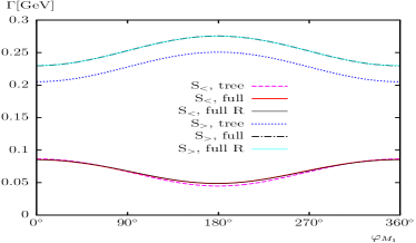
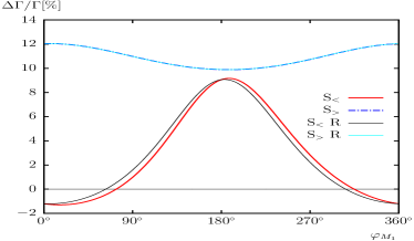
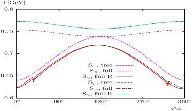
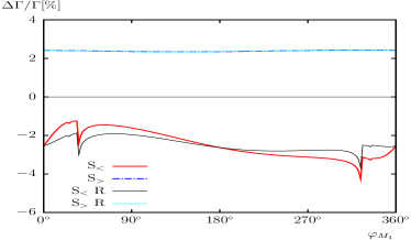
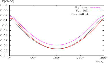
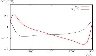
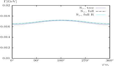
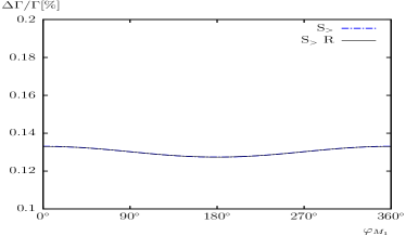
Figure 2: Tree-level (“tree”) and full one-loop (“full”) corrected decay widths are shown with $\phi_{M_{1}}$ varied. Also shown are the full one-loop corrected decay widths omitting the absorptive contributions (“full R”). First row: $\Gamma(\tilde{\chi}^{-}_{2}\to\tilde{\chi}^{0}_{1}H^{-})$, second row: $\Gamma(\tilde{\chi}^{-}_{2}\to\tilde{\chi}^{0}_{2}H^{-})$, third row: $\Gamma(\tilde{\chi}^{-}_{2}\to\tilde{\chi}^{0}_{3}H^{-})$, fourth row: $\Gamma(\tilde{\chi}^{-}_{1}\to\tilde{\chi}^{0}_{1}H^{-})$.

In Fig. 2 we show $\Gamma(\tilde{\chi}^{-}_{2}\to\tilde{\chi}^{0}_{1}H^{-})$ (first), $\Gamma(\tilde{\chi}^{-}_{2}\to\tilde{\chi}^{0}_{2}H^{-})$ (second), $\Gamma(\tilde{\chi}^{-}_{2}\to\tilde{\chi}^{0}_{3}H^{-})$ (third) and $\Gamma(\tilde{\chi}^{-}_{1}\to\tilde{\chi}^{0}_{1}H^{-})$ (fourth row) as a function of $\varphi_{M_{1}}$ for the parameters in Tab. 2, where the left (right) column displays the (relative one-loop correction to the) decay width. The decay widhts are of ${\cal O}(0.1\,\,\mathrm{GeV})$ in the case of $\tilde{\chi}^{-}_{2}\to\tilde{\chi}^{0}_{1}H^{-}$, about five times larger for $\tilde{\chi}^{-}_{2}\to\tilde{\chi}^{0}_{2,3}H^{-}$ and a factor of ten smaller for the light chargino decay. For the heavy chargino decay a strong variation with $\varphi_{M_{1}}$ can be observed. The size of the one-loop corrections, as shown in the right column, is also sizable in the case of the heavy chargino, between $-4\%$ and $+12\%$ and show a non-negligible dependence on $\varphi_{M_{1}}$. Again the effects of the “absorptive contributions” are clearly visible. Also these loop corrections should be taken into account in a reliable complex phase determination in the chargino/neutralino sector.

References

- [1]
-
[2]
H.P. Nilles,
Phys. Rept. 110 (1984) 1;
H.E. Haber and G.L. Kane, Phys. Rept. 117 (1985) 75;
R. Barbieri, Riv. Nuovo Cim. 11 (1988) 1. -
[3]
A. Pilaftsis,
Phys. Rev. D 58 (1998) 096010
[arXiv:hep-ph/9803297];
A. Pilaftsis, Phys. Lett. B 435 (1998) 88 [arXiv:hep-ph/9805373]. - [4] A. Pilaftsis and C. Wagner, Nucl. Phys. B 553 (1999) 3 [arXiv:hep-ph/9902371].
- [5] D. Demir, Phys.Rev. D 60 (1999) 055006 [arXiv:hep-ph/9901389].
- [6] S. Heinemeyer, Eur. Phys. J. C 22 (2001) 521, hep-ph/0108059.
-
[7]
TESLA Technical Design Report [TESLA Collaboration] Part 3,
“Physics at an Linear Collider”,
arXiv:hep-ph/0106315,
see: tesla.desy.de/new_pages/TDR_CD/start.html;
K. Ackermann et al., DESY-PROC-2004-01. -
[8]
J. Brau et al. [ILC Collaboration],
ILC Reference Design Report Volume 1 - Executive Summary,
arXiv:0712.1950 [physics.acc-ph];
G. Aarons et al. [ILC Collaboration], International Linear Collider Reference Design Report Volume 2: Physics at the ILC, arXiv:0709.1893 [hep-ph]. - [9] T. Fritzsche, S. Heinemeyer, H. Rzehak and C. Schappacher, arXiv:1111.7289 [hep-ph].
- [10] S. Heinemeyer, F. v.d. Pahlen and C. Schappacher, to appear in Eur. Phys. J. C, arXiv:1112.0760 [hep-ph].
- [11] S. Heinemeyer, W. Hollik and G. Weiglein, Comput. Phys. Commun. 124 (2000) 76 [arXiv:hep-ph/9812320]; see www.feynhiggs.de .
- [12] S. Heinemeyer, W. Hollik and G. Weiglein, Eur. Phys. J. C 9 (1999) 343 [arXiv:hep-ph/9812472].
- [13] G. Degrassi, S. Heinemeyer, W. Hollik, P. Slavich and G. Weiglein, Eur. Phys. J. C 28 (2003) 133 [arXiv:hep-ph/0212020].
- [14] M. Frank, T. Hahn, S. Heinemeyer, W. Hollik, R. Rzehak and G. Weiglein, JHEP 02 (2007) 047 [arXiv:hep-ph/0611326].
- [15] S. Heinemeyer, H. Rzehak and C. Schappacher, Phys. Rev. D 82 (2010) 075010 [arXiv:1007.0689 [hep-ph]]; PoSCHARGED 2010 (2010) 039 [arXiv:1012.4572 [hep-ph]].
- [16] S. Heinemeyer and C. Schappacher, arXiv:1112.2830 [hep-ph].
-
[17]
J. Küblbeck, M. Böhm and A. Denner,
Comput. Phys. Commun. 60 (1990) 165;
T. Hahn, Comput. Phys. Commun. 140 (2001) 418 [arXiv:hep-ph/0012260];
T. Hahn and C. Schappacher, Comput. Phys. Commun. 143 (2002) 54 [arXiv:hep-ph/0105349].
The program, the user’s guide and the MSSM model files are available via
www.feynarts.de . - [18] T. Fritzsche, PhD thesis, Cuvillier Verlag, Göttingen 2005, ISBN 3–86537–577–4.
- [19] T. Hahn and M. Pérez-Victoria, Comput. Phys. Commun. 118 (1999) 153 [arXiv:hep-ph/9807565].
- [20] F. del Aguila, A. Culatti, R. Munoz Tapia and M. Perez-Victoria, Nucl. Phys. B 537 (1999) 561 [arXiv:hep-ph/9806451].
-
[21]
W. Siegel,
Phys. Lett. B 84 (1979) 193;
D. Capper, D. Jones, and P. van Nieuwenhuizen, Nucl. Phys. B 167 (1980) 479. - [22] D. Stöckinger, JHEP 0503 (2005) 076 [arXiv:hep-ph/0503129].
- [23] W. Hollik and D. Stöckinger, Phys. Lett. B 634 (2006) 63 [arXiv:hep-ph/0509298].