Wave Function Renormalization Effects in Resonantly Enhanced Tunneling

Abstract

We study the time evolution of ultra-cold atoms in an accelerated optical lattice. For a Bose-Einstein condensate with a narrow quasi-momentum distribution in a shallow optical lattice the decay of the survival probability in the ground band has a step-like structure. In this regime we establish a connection between the wave function renormalization parameter $Z$ introduced in [Phys. Rev. Lett. 86, 2699 (2001)] to characterize non-exponential decay and the phenomenon of resonantly enhanced tunneling, where the decay rate is peaked for particular values of the lattice depth and the accelerating force.

I Introduction

Resonantly enhanced tunneling (RET) is a quantum effect in which the probability for the tunneling of a particle between two potential wells is increased when the quantized energies of the initial and final states of the process coincide. In spite of the fundamental nature of this effect bohm and its practical interest chang , it has been difficult to observe it experimentally in solid state structures. Since the 1970s, much progress has been made in constructing solid state systems such as superlattices chang_app ; esaki_review ; Glutsch2004 and quantum wells wagner93 which enable the controlled observation of RET leo03 .

In recent years, ultra-cold atoms in optical lattices grynberg ; rev1 , arising from the interference pattern of two or more intersecting laser beams, have been increasingly used to simulate solid state systems Bloch2005 ; rev1 ; rev2 . Optical lattices are easy to realize in the laboratory, and the parameters of the resulting one-, two- or three-dimensional periodic potentials (the lattice spacing and the potential depth) can be perfectly controlled both statically and dynamically. In the papers Sias et al. (2007); Zenesini et al. (2008), a Bose-Einstein condensate (BEC) in accelerated optical lattice potentials was used to study the phenomenon of RET. In a tilted periodic potential, atoms can escape by tunneling to the continuum via higher-lying levels. Within the RET process the tunneling of atoms out of a tilted lattice is resonantly enhanced when the energy difference between lattice wells matches the distance between the energy levels in the wells.

The atomic temporal evolution is described by the survival probability, starting from an initial state prepared in the ground band of the lattice. At long interaction times, after several tunneling processes, the survival probability is characterized by an exponential decay rate with a constant tunneling probability for each Bloch period Glueck2002 . Such a decay was examined in different theoretical analyses wagner93 ; Glutsch2004 ; Glueck2002 and measured in experimental investigations with ultra-cold atoms Sias et al. (2007); Zenesini et al. (2008); Zenesini:2009 ; Tayebirad:2010 . In this study we scrutinize the time behavior of the tunneling probability and use its remarkable features at short and intermediate times in order to extract information about wave-function renormalization effects.

The key quantity in this context is the probability that the system investigated “survives” in a given state (or a set of states, such as a band of a lattice). In this article we shall deal with survival probabilities whose behavior is complex and difficult to analyze. See for example the experimental results of ref. Zenesini:2009 and the Figs. 2 and 5 in the following, which display the survival probability of a cloud of ultra-cold atoms in the ground band of an accelerated optical lattice. Clearly, one can properly speak of the “decay” associated with an unstable system (the atoms tend to leak out of the accelerated lattice), but the time evolution can display oscillations or even plateaus. (As we shall see, the latter are easily understood in terms of the initial atomic state.)

General theoretical considerations show that the (adiabatic) survival probability of an unstable system can often be written as

$$P(t)=Z\exp\left(-\gamma t\right)+\textrm{additional contributions},$$ (1)

where $\gamma$ is the decay rate, which can be computed by the Fermi golden rule, and the parameter $Z$, representing the extrapolation of the asymptotic decay law back to $t=0$, is related to wave-function renormalization. Law (1) is valid both in quantum mechanics textbook00 ; textbook0 and quantum field theory textbook1 ; textbook2 , and $Z$ can be smaller or larger than unity Pascazio . Typically, the additional contributions in (1) dominate both at short and long times, where the exponential decay law is superseded by a quadratic Misra and Sudarshan (1977); Facchi and Pascazio (2003); temprevi and a power law Khalfin57 , respectively. They are therefore crucial in order to cancel the exponential in these time domains. However, they can play a key role in a much more general context, such as the RET phenomenon to be investigated in this article.

The pioneering experiments performed in Texas, with Landau-Zener transitions in cold atoms, checked the existence of the short-time quadratic behavior Wilkinson:1997 and the transition Fischer:2001 from the quantum Zeno effect Misra and Sudarshan (1977) to the anti- or inverse-Zeno effect Lane ; FP ; KK , through a sequence of properly tailored quantum measurements.

With the arrival of Bose-Einstein condensates the experimental resolution has advanced even further as compared to cold atoms. While cold atoms can have a momentum distribution on the order of a Brillouin zone or more, a very narrow distribution (much smaller than a Brillouin zone) is achievable with BECs. Even the steplike structure of the survival probability occuring for shallow lattice depth can be resolved with great precision Zenesini:2009 ; Tayebirad:2010 . It is in this regime of shallow lattices and short jump times Vitanov where the yet unobserved link of RET and the initial deviation from exponential decay is most striking. This work is devoted to the study of these effects. The choice of a different initial atomic state, with a well defined momentum, will enable us to observe a more complicated temporal structure. We shall therefore scrutinize the time evolution in order to unveil an exponential regime and introduce the $Z$ parameter in our RET framework.

The paper is organized as follows. We briefly sum up previous results on RET and the quantum Zeno effect in Section II. We then analyze the dynamics in the tilted lattice in Section III, and show in Section IV, the main part of this article, how the two phenomena arise as interference effects. Section V reports experimental results for the wave-function renormalization parameter $Z$ in the case of a Bose-Einstein condensate in an accelerated optical lattice, and also a comparison with the experimental configuration by Wilkinson et al. Wilkinson:1997 . Section VI concludes our work.

II Landau-Zener and resonantly enhanced tunneling

A Landau-Zener (LZ) transition takes place in a system with a time-dependent Hamiltonian, in which the spectrum, as a function of a control parameter (here time $t$), is characterized by the presence of an avoided crossing Landau ; Zener ; Stueckelberg ; Majorana ; Jones . A LZ transition is described by the following two-level Hamiltonian

$$H_{\mathrm{LZ}}(t)=\left(\begin{array}[]{cc}\alpha t&\delta E/2\\ \delta E/2&-\alpha t\end{array}\right),$$ (2)

written in a suitable basis, known as diabatic basis. The expectation values of Eq. (2) on the two states of the basis depend linearly on time and cross at $t=0$. On the other hand, the coupling $\delta E/2$ between the states is constant. The diagonalization of Eq. (2) yields the eigenvalues

$$E_{\pm}=\pm\sqrt{(\alpha t)^{2}+\left(\frac{\delta E}{2}\right)^{2}}.$$ (3)

The eigenbasis of $H_{\mathrm{LZ}}(t)$ is called the adiabatic basis. At $t\rightarrow-\infty$ the adiabatic energy levels of Eq. (3) are infinitely separated, and no transition between them occurs. The distance between the levels decreases towards the avoided crossing at $t=0$, and then increases again until, at $t\rightarrow\infty$, the separation becomes again infinite. If the system is prepared at $t\rightarrow-\infty$ in one of the adiabatic eigenstates, the probability that the system undergoes a transition at $t\rightarrow\infty$ towards the other adiabatic eigenstate reads Zener

$$P_{\mathrm{LZ}}=\exp\left(-\frac{\pi(\delta E)^{2}}{4\hbar\alpha}\right).$$ (4)

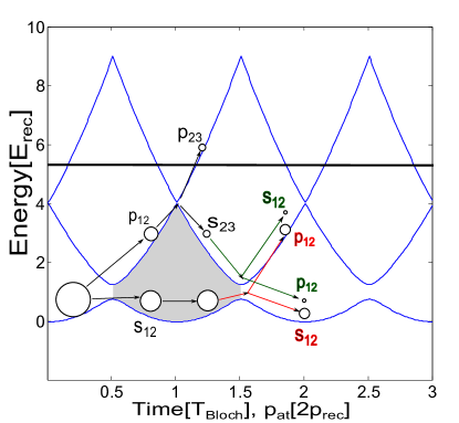
Figure 1: (color online) Energy diagram for a particle in a periodic potential vs either the time, in units of Bloch time $T_{\rm B}$ defined in (14), and the atomic momentum $p_{\mathrm{at}}/2p_{\mathrm{rec}}$ where $p_{\mathrm{rec}}=\hbar\pi/d_{L}$ units. Under the application of an external force, the quasi-momentum increases with time and at the avoided crossing between two bands, at the edge of the Brillouin zone, where $p_{\mathrm{at}}=p_{\mathrm{rec}}$, the condensate tunnels with a probability amplitude $p_{ij}$ and survives with an amplitude $s_{ij}$, defined in Eq. (22) below. Between two avoided crossings of the lowest two bands a relative phase $\phi$, defined in Eq. (17), is acquired, which is graphically displayed in the figure as a grey area. The final survival probability at a given time is the sum over all possible routes, just like a path integral in momentum space.

A particle in a shallow periodic potential, subjected to an external force, is an example of a physical system in which a LZ process can be observed. In this case, the diabatic basis is represented by the momentum eigenstates. As schematized in Fig. 1, if the system is initially prepared in the lowest band, with a very peaked momentum distribution around $p=0$, it will evolve towards the edge of the first Brillouin zone, where the distance between the first and the second band is minimal and transitions are more likely to occur, and then evolves back to the bottom of the first band. The transition probability towards the second band in this process can be approximated by $P_{\mathrm{LZ}}$, but discrepancies can arise due to the differences between the idealized case, leading to the LZ formula (4), and the real physical situation. Indeed, the periodicity of the lattice implies that the aforementioned process occurs in a finite time, and that in the initial and final states the adiabatic levels are not infinitely separated. The corrections to the LZ transition probability due to the finite duration of the process are discussed in Holthaus ; Tayebirad:2010 .

Other corrections to Eq. (4) should be considered if the lattice is not shallow. In this case, couplings to higher momentum states play an important role and a two-level description is not a good approximation anymore.

Moreover, there is another kind of deviation from LZ, which will be the main object of our analysis. Since Eq. (4) is obtained under the hypothesis that only one of the two adiabatic eigenstates is initially populated, it is not valid anymore if both states are populated. These deviations can be relevant even if one of the initial populations is very close to zero, since their order is square root of the smaller population, as will be discussed in the following. In a periodic potential, tilted by an external force $F$, the probability that a wave packet initially prepared in the first band jumps to the second band corresponds to the LZ prediction (4) only if the second band is empty. A small population in the second band gives rise to oscillations around $P_{\mathrm{LZ}}$.

Finally, the transition probability is enhanced by a large factor with respect to the LZ prediction if the energy difference $Fd_{L}\Delta i$ between two potential wells ($d_{L}$ being the lattice spacing and $d_{L}\Delta i$ the distance between the wells) matches the average band gap of the non-tilted system (RET). One expects that in a RET process from the first to the second band, the asymptotic regime will only be reached after a transient period. Indeed, while the first transition occurs when the second band is strictly empty (and thus the tunneling event closely follows the LZ prediction), further RET transitions will occur periodically in time and, starting from the second tunneling process, interference effects due to the finite population amplitude in the second band will start to play an important role, modifying the time evolution in an important way.

The analysis of the following two sections will endeavor to take all these effects into account. We shall build up an effective model, whose validity will be tested for rather diverse ranges of the parameters, and compared to experimental results finally in section V.

III Dynamics of interband tunneling

In our analysis we are interested in describing the RET process from the first to the second band of a Bose-Einstein condensate loaded into an optical lattice. It will be assumed that almost all the particles of the system are in the condensate, so that the system is described by a single-particle wave function $\psi(x,t)$ Stringari . Moreover, we will consider the condensate dilute enough so that the interaction between particles can be neglected. This implies that the wave function of the system obeys a linear Schrödinger equation. Nonlinear effects have been studied in the RET regime in previous works Sias et al. (2007); Zenesini et al. (2008); AW2011 ; Wim2005 ; WimZ1 ; WimZ2 ; WimZ3 ; WimZ4 .

The experimental condition is that of an accelerating one-dimensional optical lattice, with constant acceleration $a$. In the rest frame of the lattice, a particle of mass $m$ sitting in the lattice is subjected to an external force $F=ma$, and thus the time-independent Hamiltonian of the system in this frame of reference reads

$$H=-\frac{\hbar^{2}}{2m}\frac{\partial^{2}}{\partial x^{2}}+\frac{V}{2}\cos\left(\frac{2\pi x}{d_{L}}\right)-Fx\equiv H_{0}-Fx,$$ (5)

where $V$ is the lattice depth and the lattice period $d_{L}$ is half wavelength of the counterpropagating lasers. $H_{0}$ represents the “unperturbed” Hamiltonian, whose eigenstates are the Bloch functions

$$\phi_{\alpha,k}(x)=\mathrm{e}^{ikx}\chi_{\alpha,k}(x),$$ (6)

$$\chi_{\alpha,k}(x+d_{L})=\chi_{\alpha,k}(x),$$ (7)

$$H_{0}\phi_{\alpha,k}(x)=E_{\alpha}(k)\phi_{\alpha,k}(x),$$ (8)

with $\alpha=1,2,3,\dots$ the band index and $k$ the quasi-momentum, ranging in the first Brillouin zone $\mathcal{B}=\{k|-\pi/d_{L}\leq k\leq\pi/d_{L}\}$. The dynamics of the system depends on two dimensionless parameters Tayebirad:2010 , related to lattice depth and external force:

$$V_{0}=\frac{V}{E_{\mathrm{rec}}},F_{0}=\frac{Fd_{L}}{E_{\mathrm{rec}}},\text{ with }E_{\mathrm{rec}}=\frac{\hbar^{2}}{2m}\left(\frac{\pi}{d_{L}}\right)^{2},$$ (9)

where $m$ is the mass of the atoms. Applying the unitary transformation

$$\tilde{\psi}(x,t)=\exp(-iFxt/\hbar)\psi(x,t)$$ (10)

restores the translational invariance of the Hamiltonian, at the expense of an explicit time dependence:

$$\tilde{H}(t)=\frac{1}{2m}\left(-i\hbar\frac{\partial}{\partial x}+Ft\right)^{2}+\frac{V}{2}\cos\left(\frac{2\pi x}{d_{L}}\right).$$ (11)

Rewriting this Hamiltonian in the momentum basis as in Tayebirad:2010 establishes the relation to the Landau-Zener Hamiltonian introduced in Eq. (2): To calculate the time evolution of any momentum eigenstate, we only need the Hamiltonian $H_{k_{0}}$ acting on the subspace with a given quasi-momentum $k_{0}$, as there is no transition between states with different $k_{0}$

$$H_{k_{0}}=\frac{1}{2m}\left(\begin{array}[]{ccccc}\ddots&&&&0\\ &\hbar^{2}(k-\frac{2\pi}{d_{L}})^{2}&mV/2&&\\ &mV/2&(\hbar k)^{2}&mV/2&\\ &&mV/2&\hbar^{2}(k+\frac{2\pi}{d_{L}})^{2}&\\ 0&&&&\ddots\\ \end{array}\right)\ ,$$ (12)

where $k=k(t)=k_{0}+Ft/\hbar$. This Hamiltonian (12) leads to a very accurate numerical solution of the Schrödinger equation. For small $V$ on the scale of $E_{\mathrm{rec}}$ its dynamics is well described by successive Landau-Zener transitions, occuring whenever two diagonal terms in $H_{k_{0}}$ become degenerate. We will use this approximation to obtain analytical results. In Fig. 1 the relevant transitions are depicted graphically.

We first examine an adiabatic approximation of the dynamics generated by the Hamiltonian (5), yielding no transition between bands (single-band approximation), which will highlight the time periodicity of the system and the phase differences between bands. We shall then introduce an effective coupling between the low-lying bands that enables one to obtain transition rates. The adiabatic approximation is consistent if $Fd_{L}\lesssim V$, namely if $F_{0}\lesssim V_{0}$ in Eq. (9).

The initial state will be assumed to be highly peaked around a single quasi-momentum value $k_{0}$, that is, the width of the initial quasi-momentum distribution will be taken to be much smaller than the width $2\pi/d_{L}$ of the first Brillouin zone $\mathcal{B}$. In this situation, it can be proved Jones ; Holthaus that in the adiabatic single-band approximation the average quasi-momentum evolves semiclassically, so that at time $t$

$$k(t)=k_{0}+\frac{Ft}{\hbar},$$ (13)

with negligible spread in the quasi-momentum distribution occurring during the evolution. This yields Bloch oscillations in a tilted lattice with a Bloch period

$$T_{\rm B}=\frac{2\pi\hbar}{Fd_{L}}=\frac{\hbar}{E_{\mathrm{rec}}}\frac{2\pi}{F_{0}}.$$ (14)

The initial state analyzed here has a well defined initial momentum (in $\mathcal{B}$), but can be distributed among different bands. At the end of each Bloch period, the amplitude in band $\alpha$ acquires the following phase with respect to the amplitude in band $\beta$

$$\Delta\varphi_{\alpha\beta}=-\frac{1}{\hbar}\langle E_{\alpha}(k)-E_{\beta}(k)\rangle T_{\rm B}=-\frac{2\pi}{F_{0}}\langle\epsilon_{\alpha}(k)-\epsilon_{\beta}(k)\rangle,$$ (15)

where $\langle\dots\rangle$ denotes the average over $\mathcal{B}$ and $\epsilon_{\gamma}(k)$ is the energy of the state with quasi-momentum $k$ in band $\gamma$ in units $E_{\mathrm{rec}}$.

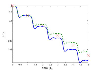
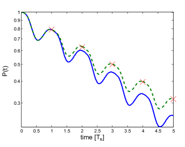
Figure 2: (color online) Adiabatic survival probability in the lowest band $P(t)$ vs. time, obtained by numerically solving the Schrödinger equation for the atomic evolution under the Hamiltonian of Eq. (11). The initial state has initial quasi-momentum $0.2p_{\textrm{rec}}$ in the Brillouin zone and a negligible quasi-momentum width. Upper panel: $V_{0}=1.5,\phi\simeq 4\pi$; lower panel: $V_{0}=4.5,\phi\simeq 2\pi$. The solid (blue) line represents the unperturbed time evolution, the dashed (green) line the time evolution with the phase change discussed in Sec. V.2 after each Bloch period. The red crosses are an extrapolation of the first time step to the following periods. Plateaus manifest for $V_{0}=1.5$ (upper panel). The validity of this picture is discussed in the text and in Appendix A.

We now analyze inter-band transitions through an effective model. We focus on the experimental parameters of the Pisa setup Zenesini:2009 ; Tayebirad:2010 and model transitions from the first to the second band. In the parameter regime of shallow lattices there is numerical and experimental evidence of a step-like structure of the adiabatic survival probability $P(t)$ Zenesini:2009 in the first band. If the initial state is peaked around $k=0$ and lies in the first band, the survival probability is characterized by steep drops around times $t=T_{\rm B}(n+1/2)$ with $n$ integer, and flat plateaus between these times Wim2005 . This view is corroborated by numerical simulations (Fig. 2, upper panel) and experimental observations Zenesini:2009 . This time evolution is due to the fact that the coupling between the first and the second band is maximal at the edge of the first Brillouin zone, for $k=\pm\pi/d_{L}$, and thus significant transitions occur there, with periodicity $T_{\rm B}$. Figure 2 shows that plateaus are clearly present for $V_{0}=1.5$ (shallow lattice, upper panel), but start to wash out for $V_{0}=4.5$ (lower panel). The range of validity of the plateau picture is further discussed in Appendix A and is approximately valid for $V_{0}\lesssim 4.5$. In the following analysis we shall focus on this regime.

The approximated dynamics takes into account experimental and numerical evidence and is valid for small values of $V_{0}$ and $F_{0}$, when the transition times can be considered much smaller than $T_{\rm B}$. We assume that the evolution inside the first band is adiabatic for all $k$, except for $k\simeq\pi/d_{L}$, when a transition towards the state with the same quasi-momentum in the second band becomes possible. This transition will be effectively described by the evolution operator of the form

$$\tilde{U}=\left(\begin{array}[]{cc}s_{12}&-p_{12}\\ p_{12}&s_{12}\end{array}\right)\,,$$ (16)

with $p_{12}=\sqrt{1-s_{12}^{2}}$. The operator $\tilde{U}$ acts on the two-dimensional space spanned by $\{\mathinner{|{1}\rangle},\mathinner{|{2}\rangle}\}$, where $\mathinner{|{1}\rangle}$ represents the state with $k=\pi/d_{L}$ in the first band and $\mathinner{|{2}\rangle}$ the state with same quasi-momentum in the second band.

The transition from the second to the third band can be schematized as the loss of a fraction $1-s_{23}^{2}$ in the population of the second band towards a continuum, occurring at the crossing around $k=0$. This assumption is justified for small values of $V_{0}$ (see discussion above), such that a particle in the third (or higher) band can be considered free.

During each Bloch cycle separating two successive transitions, the relative phase between the second and the first band amplitudes increases by (15), which reads

$$\phi(V_{0},F_{0})=\frac{2\pi}{F_{0}}\langle\Delta E(V_{0})\rangle,$$ (17)

where $\langle\Delta E\rangle$ is the energy difference (in units $E_{\mathrm{rec}}$) between the second and the first band, averaged over $\mathcal{B}$. This quantity can be exactly computed by using Mathieu characteristics $a(\kappa,q)$, which are the eigenvalues of the Mathieu equation Poole

$$\frac{d^{2}y}{dx^{2}}+\left[a-2q\cos(2x)\right]y=0,$$ (18)

corresponding to the Floquet solutions $y(x)=\exp(i\kappa x)u(x)$. For small $V_{0}$, a good estimate is given by a Landau-Zener gap integration

$$\langle\Delta E\rangle\simeq\frac{1}{4}\sqrt{64+V_{0}^{2}}+\frac{V_{0}^{2}}{32}\mathrm{arcsinh}\frac{8}{V_{0}}.$$ (19)

For larger $V_{0}$, a tight-binding, or harmonic oscillator, approximation yields

$$\langle\Delta E\rangle\simeq\sqrt{4V_{0}}-1.$$ (20)

The exact result and the two aforementioned approximations are compared in Fig. 3.

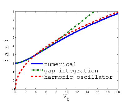
Figure 3: (color online) Average band gap $\langle\Delta E\rangle$ vs $V_{0}$, both in $E_{\mathrm{rec}}$ units. Comparison between numerical results, analytical results from Eq. (19), and the harmonic oscillator approximation (20). In the small $V$ regime the band integration yields a good approximation, while for larger $V$, where the coupling becomes continuous, the harmonic oscillator approximation is more effective.

The effects of the dynamics in a time $T_{\rm B}$ from one transition to the next one can thus be modelled in the basis $\{\mathinner{|{1}\rangle},\mathinner{|{2}\rangle}\}$ by an effective non-unitary operator

$$W=\left(\begin{array}[]{cc}1&0\\ 0&s_{23}\mathrm{e}^{i\phi}\end{array}\right).$$ (21)

By making use of this simplified model, we describe the time evolution in the following way. At $t=0$ the condensate is in the first band, with quasi-momentum close to $k=0$. As the lattice is accelerated, the quasi-momentum increases until it reaches $\pi/d_{L}$ at $t=T_{\rm B}/2$, where the operator $\tilde{U}$ comes into play and transfers part of the population to the second band. The evolution from $T_{\rm B}/2$ to $3T_{\rm B}/2$ is summarized by the application of $W$. Then, the second transition occurs, and part of the population in the second band (decreased by losses towards the third band) can tunnel back to the first band due to the action of $\tilde{U}$ and gives rise to interference effects. The same steps occur in the subsequent transitions.

On a time span $T_{\rm B}$, the dynamics of the system is therefore determined by the successive action of the non-unitary operator

$$U=\tilde{U}W=\left(\begin{array}[]{cc}s_{12}&-p_{12}s_{23}\mathrm{e}^{i\phi}\\ p_{12}&s_{12}s_{23}\mathrm{e}^{i\phi}\end{array}\right)$$ (22)

in the basis $\{\mathinner{|{1}\rangle},\mathinner{|{2}\rangle}\}$. The order of the two operations is not relevant, since $W$ acts trivially on the “initial state” $\mathinner{|{1}\rangle}$ before the first transition.

Besides the phase $\phi$, the operator $U$ depends on two other independent parameters, namely the survival amplitudes $s_{12}$ and $s_{23}$. $s_{12}$ represent the survival amplitude in the first band after the first transition, which is in fact comparable to a LZ process since the second band is initially empty. The survival probability $s_{23}$ is related to a LZ tunneling from the second to the third band, if we assume the third band to be empty before each transition process. A graphical representation of the parameters appearing in Eq. (22) is given in Fig. 1.

Using the LZ critical acceleration for the first and second band gap Landau ; Zener ; Niu et al. (1996); Iliescu et al. (1992), analytical expressions for $s_{12}$ and $s_{23}$ as functions of the microscopic parameters can be obtained. At lowest order in $V_{0}$, the survival amplitudes read

$$s_{12}(V_{0},F_{0}) = \sqrt{1-P_{\mathrm{LZ}}^{(1,2)}(V_{0},F_{0})}$$ (23)

$$= \sqrt{1-\exp\left(-\frac{\pi^{2}V_{0}^{2}}{32F_{0}}\right)},$$

$$s_{23}(V_{0},F_{0}) = \sqrt{1-P_{\mathrm{LZ}}^{(2,3)}(V_{0},F_{0})}$$ (24)

$$= \sqrt{1-\exp\left(-\frac{\pi^{2}V_{0}^{4}}{32\cdot 16^{2}(2F_{0})}\right)},$$

where $P_{\mathrm{LZ}}^{(i,j)}$ is the Landau-Zener transition probability (4) from band $i$ to band $j$.

The evolution on a timescale $T_{\rm B}$, determined by a sequence of $U$ operations, will be analyzed in detail in the following section.

IV Transient and asymptotic behavior

We now specialize the model outlined in Section III to the Pisa experimental setup Zenesini:2009 ; Tayebirad:2010 . The state of the system before the first transition is $\mathinner{|{1}\rangle}$. Immediately after the $n$-th transition, occurring at time $t=T_{\rm B}(n+1/2)$, the state of the system is

$$\mathinner{|{\Phi_{n}}\rangle}=U^{n}\mathinner{|{1}\rangle}.$$ (25)

The matrix $U$ in Eq. (22) can be diagonalized, yielding eigenvalues $(e_{1},e_{2})$. By expanding the initial state as

$$\mathinner{|{1}\rangle}=c_{1}\mathinner{|{\psi_{1}}\rangle}+c_{2}\mathinner{|{\psi_{2}}\rangle},$$ (26)

where $\mathinner{|{\psi_{1,2}}\rangle}$ are the normalized non-orthogonal eigenvectors of $U$, the state of the system at time $T_{\rm B}(n+1/2)$ is

$$\mathinner{|{\Phi_{n}}\rangle}=c_{1}e_{1}^{n}\mathinner{|{\psi_{1}}\rangle}+c_{2}e_{2}^{n}\mathinner{|{\psi_{2}}\rangle}.$$ (27)

Due to the dissipative term in $W$, the two eigenvalues are smaller than unity, and one of them, say $e_{1}$, is larger in modulus than the other one. Thus, for $n$ sufficiently large, the evolution reaches an asymptotic regime, in which the state after the $n$-th transition is determined only by the state after the previous one, with a transition rate depending on the largest eigenvalue. Since the survival probability in the first band can be defined as $P_{n}=|\langle 1|\Phi_{n}\rangle|^{2}$, in the asymptotic regime one gets

$$P_{n}\simeq|e_{1}|^{2}P_{n-1}.$$ (28)

By defining an asymptotic transition rate

$$\gamma=-\log\left(|e_{1}|^{2}\right),$$ (29)

it is possible to introduce a function $P_{\rm Z}(t)$ that coincides with the value of the survival probability at the center of the plateaus, at times $t=nT_{\rm B}$:

$$P_{\rm Z}(t)=Z\exp\left(-\gamma t\right).$$ (30)

Compare with Eq. (1). The parameter $Z$ in Eq. (30) is in general different from unity, due to the transient regime at the beginning of the evolution. It represents the extrapolation of the asymptotic exponential probability back at $t=0$.
We now derive an analytical expression for $Z$. In the asymptotic regime, the system evolution described by Eq. (27) corresponds to an evolution operator applied to an initial unnormalized vector $\mathinner{|{\Psi_{0}}\rangle}\equiv c_{1}\mathinner{|{\psi_{1}}\rangle}$:

$$\mathinner{|{\Phi_{n}}\rangle}\simeq c_{1}e_{1}^{n}\mathinner{|{\psi_{1}}\rangle}=U^{n}\left(c_{1}\mathinner{|{\psi_{1}}\rangle}\right)=U^{n}\mathinner{|{\Psi_{0}}\rangle}.$$ (31)

The $Z$ parameter, representing the extrapolation of the asymptotic behavior back to $t=0$, can be defined as the square modulus of the projection of the fictitious initial vector $\mathinner{|{\Psi_{0}}\rangle}$, onto the actual initial state $\mathinner{|{1}\rangle}$

$$Z\equiv|\mathinner{\langle{1}|}\Psi_{0}\rangle|^{2}=|c_{1}|^{2}|\mathinner{\langle{1}|}\psi_{1}\rangle|^{2},$$ (32)

which corresponds to an extrapolated “survival probability” in the subspace spanned by $\mathinner{|{1}\rangle}$, evaluated at the initial time. $Z$ can be analytically computed as a function of the independent parameters of the model, by explicitly diagonalizing $U$. One obtains

$$Z(s_{12},s_{23},\phi)=\frac{\left[\frac{s_{12}}{2}(1-s_{23}\cos\phi)+\sqrt{\frac{\mathcal{K}(s_{12},s_{23},\phi)}{8}}\right]^{2}+s_{23}^{2}\sin^{2}\phi\left[\frac{2-s_{12}^{2}(1+s_{23}\cos\phi)}{\sqrt{2\mathcal{K}(s_{12},s_{23},\phi)}}+\frac{s_{12}}{2}\right]^{2}}{\frac{\mathcal{K}(s_{12},s_{23},\phi)}{2}+\frac{2s_{23}^{2}\sin^{2}\phi}{\mathcal{K}(s_{12},s_{23},\phi)}\left[2-s_{12}^{2}(1+s_{23}\cos\phi)\right]^{2}},$$ (33)

with

$$\mathcal{K}(s_{12},s_{23},\phi) = s_{12}^{2}\left(1+2s_{23}\cos\phi+s_{23}^{2}\cos(2\phi)\right)-4s_{23}\cos\phi$$ (34)

$$+\sqrt{s_{12}^{4}\left(1+2s_{23}\cos\phi+s_{23}^{2}\right)-8s_{23}s_{12}^{2}\left(\cos\phi+2s_{23}+s_{23}^{2}\cos\phi\right)+16s_{23}^{2}}.$$

In order to gain a qualitative understanding of the dependence of $Z$ (and $\gamma$) on the phase difference $\phi$ acquired during a Bloch cycle, let us compare the first and second transitions. Let $P_{0}=1$ be the initial value of the survival probability in the first band. After the first transition, the survival probability becomes

$$P_{1}=s_{12}^{2}P_{0}\equiv\mathrm{e}^{-\gamma_{0}}P_{0}.$$ (35)

At the second transition, the discrepancy with the LZ prediction becomes manifest. Since, in the parameter regime of small $V_{0}$ we are considering, the ratio $s_{23}/s_{12}$ is very small [see Eqs. (23)-(24)], we can apply a first-order approximation, yielding

$$P_{2}\simeq(s_{12}^{2}-2s_{23}p_{12}^{2}\cos\phi)P_{1}\equiv\mathrm{e}^{-\gamma_{1}}P_{1}.$$ (36)

Thus, if the phase is $\phi=2\pi j$, with $j\in\mathbb{Z}$, the second transition is enhanced with respect to the first one. In this case, a local maximum in the transition rate as a function of $F_{0}$ is expected. On the contrary, if $\phi=(2j+1)\pi$, the second transition is less pronounced than the first one.

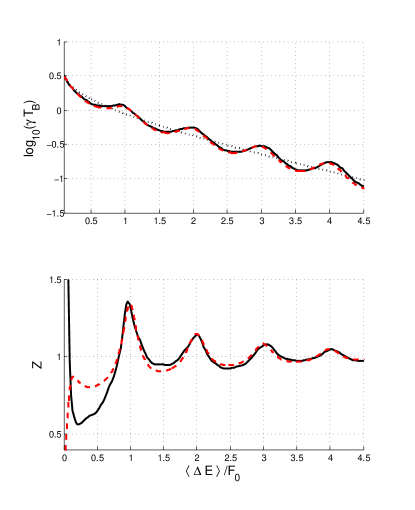
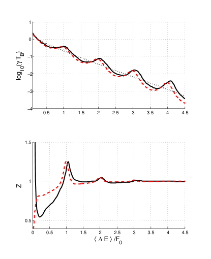
Figure 4: (color online) Decay rate $\gamma$ and wave-function renormalization $Z$ vs $\langle\Delta E\rangle/F_{0}=\phi/2\pi$. Comparison among analytical results, obtained by exact diagonalization of the reduced evolution operator $U$ in Eq. (22) [(red) dashed lines], numerical simulations based on Eq. (11) (solid lines) and Landau-Zener prediction (dotted lines for $\gamma$). Upper two panels: $V_{0}=2$; lower two panels: $V_{0}=4$.

A backwards extrapolation of the second step gives a rough estimate of the $Z$ parameter, which we call $Z_{1}$:

$$Z\simeq Z_{1}=\mathrm{e}^{\gamma_{1}-\gamma_{0}}\simeq 1+2s_{23}\left(\frac{p_{12}}{s_{12}}\right)^{2}\cos\phi.$$ (37)

Even if Eq. (37) represents a rather crude approximation, it brings to light the correspondence between resonances in the asymptotic transition rates and resonances in the $Z$ parameter. Quantities like (37) are very useful in an experimental context, where only the first few steps in the Bloch cycles are accessible. If the survival amplitude can be measured up to the $N$-th transition, the $Z$ parameter can be approximated by

$$Z\simeq Z_{N}=\mathrm{e}^{N\gamma_{N}-\sum_{n=0}^{N-1}\gamma_{n}}.$$ (38)

At the same time,

$$\gamma\simeq\gamma_{N}.$$ (39)

The convergence to the real value of $Z$ is typically very fast, and the first few cycles are already sufficient to obtain an excellent approximation.

The estimates of Eqs. (17)-(23), together with Eq. (33) enable one to obtain an analytical expression $Z(V_{0},F_{0})$, yielding the value of $Z$ as a function of the microscopic parameters. Figure 4 shows a comparison of the numerical calculation and the estimates for $\gamma$ and $Z$ with our analytical model. It is clear that the model yields a better approximation for smaller $V_{0}$. For $V_{0}\gtrsim 4.5$ the peaks of $Z$ are overestimated and the picture of successive tunneling events with an intermediate phase accumulation becomes less valid. In the regime of small $V_{0}$, the analytical model is very efficient, as long as $F_{0}$ is not too large and the LZ tunneling rates do not have to be adjusted due to the finite initial time of the evolution Holthaus .

V Experimental configurations

This section contains a discussion of the experiments performed up to now and suggestions for future measurements aimed at controlling the decay by a manipulation of the phase of the temporally evolved atomic wave packet. The relations of Sec. IV can be tested experimentally as follows.

V.1 Measurement of $P(t)$

An experimental check of the theory at the basis of the wave-function renormalization $Z$ is obtained by measuring the survival probability $P(t)$ for a time up to five Bloch periods for different parameter values, as in Fig. 2, and then introducing a fit with the exponential law of Eq. (30) for the survival probability at times $t=nT_{\rm B}$. The $Z$ and $\gamma$ parameters are determined by such a fit. The results of this approach are discussed in the following for the case of a narrow atomic momentum distribution, as in the RET experiments at Pisa with a Bose-Einstein condensate Tayebirad:2010 ; Sias et al. (2007); Zenesini et al. (2008); Zenesini:2009 , and for the case of a broad atomic momentum distribution, as for the experiment performed at Austin Wilkinson:1997 ; Fischer:2001 .

V.1.1 Pisa RET experiment

The time dependence of the adiabatic survival probability was measured by freezing the tunneling process through projective quantum measurements on the states of the adiabatic Hamiltonian Zenesini:2009 . Experimental results of $P(t)$ for different values of the lattice depth and the applied force are shown in Fig. 5. The solid and dashed lines are a numerical simulation of our experimental protocol and an exponential decay fit for our system’s parameters, respectively. The vertical intercept of the exponential decay at $t=0$ gives the value of and the exponential decay rate gives the value of $\gamma$.
The resonant tunneling appears as a strong variation for the exponential decay rate of $\gamma$ as a function of $\phi$, as measured in the experiments Sias et al. (2007); Zenesini et al. (2008). This variation matches the numerical predictions of Fig. 4.
Measured values of the $Z$ parameter vs the $\phi$ parameter are plotted in Fig. 6(a). The error bars on the $Z$ values are determined by the exponential fits, as in Fig. 5. Notice that $Z$ values both larger and smaller than one are measured. The error of the phase $\phi$ is linked to the experimental accuracy of the $V_{0}$ and $F_{0}$ parameters ($V_{0}$ carries an error of around ten percent). The experimental results are compared to theoretical predictions for the numerical solutions of the time-dependent adiabatic survival probability. The peaks in the plot are determined by RET resonances. The simulation of Fig. 4 evidences that the dependence of $Z$ on $\phi$ matches the dependence of $\gamma$. The position of the largest peak corresponds to the main resonance Sias et al. (2007); Zenesini et al. (2008) $\Delta i=1$, and the positions of the smaller peaks are in agreement with those of higher order resonances. The agreement between the theoretical and experimental determinations of $Z$ is very good, taking in account the difficulties of a precise determination of the lattice depth $V_{0}$. It should be noticed a posteriori that the experimental results are more easily produced in the case $Z<1$.

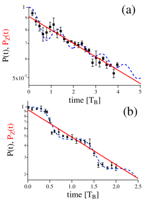
Figure 5: (color online) $P(t)$: experimental results (squares) and numerical solution of the Schrödinger equation describing the atomic cloud within the accelerated optical lattice (blue dashed line). The (red) continuous lines are exponential fits to the experimental data based on $P_{\rm Z}(t)$ by Eq. (30), whose crossing with the $y$ axis yields the value of $Z$. In (a) $V_{0}=5.8E_{\textrm{rec}}$, $F_{0}=5$ and in (b) $V_{0}=1E_{\textrm{rec}}$, $F_{0}=0.383$. Both cases yield $Z<1$. The slope of the exponential decay gives the decay rate $\gamma$.

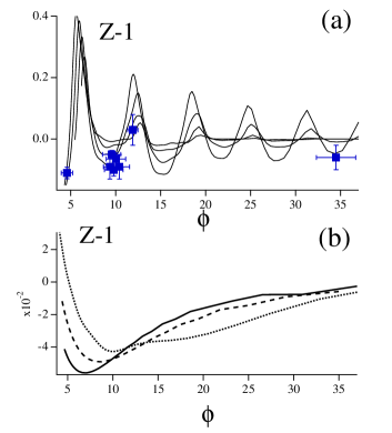
Figure 6: (a) Scaling plot of $Z-1$ vs. $\phi$ of Eq. (17), derived from RET experimental results (squares) using a narrow atomic quasi-momentum distribution. The experimental point at $\phi=4.8$ is obtained from the data of Fig. 5(a) and the point at $\phi=34$ from the data of Fig. 5(b). Full lines are the theoretical predictions for $V_{0}=1,2,3,4$. The RET coupling yields the oscillating behavior of $Z$ vs $\phi$, with the oscillation amplitudes increasing at lower $V_{0}$ for a fixed $\phi$. (b) Theoretical prediction for $Z-1$ in an Austin-type experiment, with a broad atomic quasi-momentum distribution, at $V_{0}=3,3.5$ and $4$ (continuous, dashed and dotted line, respectively).

V.1.2 Austin experiment on non-exponential decay

The very broad atomic distribution of the experiment perfomed by Raizen’s group in Texas Wilkinson:1997 ; Fischer:2001 , occupying several Brillouin zones, leads to a different temporal evolution of the survival probability. In particular, the deeper lattice potentials used in these works imply a different behavior of the $Z$ function. The survival probability was numerically evaluated on the basis of the theoretical treatment reported in Niu and Raizen Niu:1998 and Wilkinson et al. Wilkinson:1997 . For the case of Rb atoms and parameters very close to those experimentally investigated in Pisa, Fig. 6(b) reports the $Z$ function versus the parameter $\phi$ at a fixed value of the lattice depth. It may be noticed that the values of $|Z-1|$ are smaller than those measured in the case of a narrow atomic quasi-momentum distribution. The $Z$ dependence on $F_{0}$ is very smooth, without the oscillations of Fig. 6(a). The Niu-Raizen theory Niu:1998 ; Wilkinson:1997 includes only the two lowest energy bands and does not take into account tunneling phenomena such as RET or higher excited energy bands. The Niu-Raizen model is thus essentially a two-state model for Landau-Zener coupling, neglecting resonant tunneling effects, and averaged over all quasi-momenta in the entire Brillouin zone. Such a model is better suited for large values of $V_{0}$, when the energy bands become flat.

V.2 Phase control

To further verify that the phase $\phi$ is, indeed, the important quantity determining the temporal evolution of the atomic wave function, it could be interesting to perform a LZ experiment for which the atomic acceleration is stopped after each Bloch period for a time $t_{\mathrm{halt}}=\pi/\Delta E$, with $\Delta E$ the energy difference between the two bands, in order to reverse the phase of the wave function’s evolution. Differences in the predicted time dependence of $P(t)$ with and without this phase reversal are reported in Fig. 2. Even if the experimental error introduced by the phase imprinting could be too large to derive $Z$ precisely in this regime, the observation of a modified decay rate in the presence of a phase reversal would represent a direct proof that $\phi$ is responsible for the resonances in the decay rate.

The survival probability obtained in an experiment where after each period one halts or does not halt, with equal probability, represents another tool for modifying and testing the interference in successive Landau-Zener processes. The change of the decay rate by this randomization is equivalent to the change that would be obtained via bona fide quantum measurements, as in the standard formulation of the Zeno effect which was experimentally oberved in Fischer:2001 . It can be demonstrated that the same atomic evolution is obtained by performing non-destructive survival probability measurements after each Bloch period, the quantum Zeno effect being achieved in the limit of very frequent measurements carried out within a Bloch period.

V.3 Emptying the second band

A similar interesting experimental configuration is realized by totally eliminating the second band’s occupation after each Bloch period. This could be produced as in the measurement protocol used in Ref. Zenesini:2009 , by decreasing the acceleration after each tunneling event from the ground band down to a small value such that the population in the second band tunnels to the continuum and is not confined anymore by the optical lattice. At the same time the population in the lower band does not tunnel to the second one, and is ready to be accelerated once again with the original large value. In this kind of setup all Landau-Zener steps in the survival probability as a function of time would have the same height on a logarithmic scale, determined by $s_{12}$ only. The phase $\phi$ would then be totally irrelevant for the atomic evolution.

V.4 Links with quantum field theory

Finally, from a theoretical perspective, it would be of great interest to explore the links with wave-function renormalization effects in quantum field theory. In that context, the quantity $Z$ arises from an analysis of the propagator (enforcing probability conservation in the Källén-Lehmann representation KL ; KL2 ) and differs from unity at second order in the coupling constant. $Z$ is smaller than unity for stable states, but is unconstrained and can become $>1$ for an unstable state. There have been a few attempts joichimatsu ; hydrovanH ; QFTC ; BMT ; AESG ; giacosapagliara1 ; giacosapagliara2 to analyze the quantum Zeno effect in the decay of elementary particles, but no experiment has been performed so far. It would be interesting to try and mimic these effects by making use of RET in BECs. This would take us into the realm of quantum simulations.

VI Conclusion and Outlook

In the pioneering work by Raizen et al. Wilkinson:1997 ; Fischer:2001 the focus was on the deviations from exponential decay and the occurrence of the quantum Zeno effect and its inverse FP ; KK due to repeated measurements. In the present article we endeavored to go further and studied Landau-Zener transitions Landau ; Zener under very different physical conditions, both in terms of initial state and parameters. This enabled us to use these effects as a benchtest for the study of wave-function renormalization effects in quantum mechanics. We have seen that by scrutinizing the features of the survival probability of the wave function that collectively describes an ultra-cold atomic cloud, one can consistently define $Z$ and extract crucial information on its behavior. It is remarkable that $Z$ can be directly measured and that its deviation from unity yields directly measurable consequences on the experimental observables. In addition, as the experimental parameters are varied, $Z$ takes values that can be smaller or larger than unity. If $Z<1$, the decay can be slowed down (quantum Zeno effect) or enhanced (anti- or inverse-Zeno effect), but if $Z>1$, only the quantum Zeno effect is possible Pascazio .

Our analysis of the atomic evolution in terms of successive free evolutions and tunneling processes, with interference in the population occupations, points out that Landau-Zener transitions and Stückelberg oscillations Stueckelberg are two facets (one could say particular cases) of the very complex problem of the atomic evolution within the periodic potential produced by the optical lattice, in analogy to a previous analysis by Kling et al. Kling:2010 .

For the shallow lattice regime, we have established a relationship between $\gamma$, $Z$ and $\phi=2\pi\langle\Delta E(V_{0})\rangle/F_{0}$. We have demonstrated that the Zeno regime and resonantly enhanced tunneling are both controlled by the same parameter $\phi$ in an ultra-cold atomic cloud. The resonances in $Z$ can be explained by a decay following the Landau-Zener probability in the first Bloch period and resonantly enhanced decay in the following periods. In contrast, the Niu-Raizen description Niu:1998 applied to describe the non-exponential decay of cold atoms in an optical lattice approximates the tunneling rate from the second to the third band by one complete decay. In the large $V_{0}$ parameter regime the RET resonances are not important and do not affect the quantum Zeno effect.

A future experiment could involve a BEC atomic cloud in the presence of atomic interactions niu ; JonaLasinio:2003 ; Sias et al. (2007); Zenesini et al. (2008); AW2011 ; Wim2005 ; WimZ1 ; WimZ2 ; WimZ3 ; WimZ4 . As verified experimentally JonaLasinio:2003 , in this case the tunneling probabilities are not symmetric ($s_{ij}\neq s_{ji}$) and the effect of the RET resonances could be enhanced or suppressed with attractive or repulsive interactions.

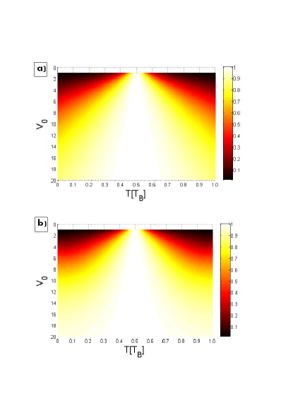
Figure 7: (color online) Adiabatic coupling strength $c(t)$ defined in Eq. (43) and normalized to maximal coupling plotted vs. time and optical lattice depth. Comparison between Lorentzian ansatz (upper panel) and numerical results based on Eq. (11) (lower panel). The assumption of short tunneling events at the avoided crossings is valid for $V_{0}\lesssim 4.5$ (shallow lattice).

Appendix A Check on the interrupted atomic evolution

The dynamics of interband tunneling is discussed in Sec. III and hinges on the assumption of a free phase evolution over the Brillouin zone, interrupted by a very short tunneling event at the avoided crossing, at well defined times $t=T_{\rm B}(n+1/2)$ with $n\in\mathbb{N}$, as in upper panel of Fig. 2 and in Fig. 5(b). To check the validity of this assumption we use the Hamiltonian $H_{a}$ which describes the time evolution in the adiabatic (energy) basis. $H_{a}$ can be obtained by expanding the state $\mathinner{|{\psi(t)}\rangle}$ of the system in the time-dependent energy basis

$$\mathinner{|{\psi(t)}\rangle}=\sum_{n}a_{n}(t)\mathinner{|{n(t)}\rangle}$$ (40)

and applying the Schrödinger equation $i\partial_{t}\mathinner{|{\psi}\rangle}=H\mathinner{|{\psi}\rangle}$ with the Hamiltonian of Eq. (12) to obtain

$$i\sum_{n}\left(\dot{a}_{n}\mathinner{|{n}\rangle}+a_{n}\partial_{t}\mathinner{|{n}\rangle}\right)=\sum_{n}a_{n}E_{n}\mathinner{|{n}\rangle}.$$ (41)

Taking the inner product with $\mathinner{\langle{m}|}$ and using $\mathinner{\langle{m|n}\rangle}=\delta_{mn}$ we get

$$\dot{a}_{m}=-iE_{m}a_{m}-\sum_{n}\mathinner{\langle{m}|}\partial_{t}\mathinner{|{n}\rangle}a_{n}$$ (42)

and see that the off-diagonal term coupling the lowest two energy states is given by

$$c(t):=\mathinner{\langle{1}|}\partial_{t}\mathinner{|{2}\rangle}.$$ (43)

In the ideal Landau-Zener model of equation (2) and Ref. Vitanov this yields for $c(t)$ a Lorentzian function of time in a narrow time interval centered around the $T_{\rm B}/2$ transition time. The Lorentzian is displayed in Fig. 7(a) for different values of the potential depth $V_{0}$. Figure 7(b) shows the numerical result for $c(t)$ in our system. The model discussed in Sec. III ceases to be valid when $c$ is large, at the border of the Brillouin zone. A comparison of the two plots in Fig. 7 clarifies that the approximations used in our analysis break down for $V_{0}\gtrsim 4.5$.

References

- (1) D. Bohm, Quantum Theory p. 286 (Dover Publications, New York, 1989).
- (2) L.L. Chang, E.E. Mendez, and C. Tejedor (eds), Resonant Tunneling in Semiconductors (Plenum, New York, 1991).
- (3) L.L. Chang, L. Esaki, and R. Tsu, Appl. Phys. Lett. 24, 593 (1974).
- (4) L. Esaki, IEEE Journal Quant. Electr. QE-22(9), 1611 (1986).
- (5) S. Glutsch, Phys. Rev. B 69, 235317 (2004).
- (6) M. Wagner and H. Mizuta, Phys. Rev. B 48, 14393 (1993).
- (7) K. Leo, High-Field Transport in Semiconductor Superlattices. (Springer, Berlin, 2003).
- (8) G. Grynberg and C. Robilliard, Phys. Rep. 355, 335 (2001).
- (9) O. Morsch and M. Oberthaler, Rev. Mod. Phys. 78, 179 (2006).
- (10) I. Bloch, Nature Physics 1, 1 (2005).
- (11) I. Bloch, J. Dalibard, and W. Zwerger, Rev. Mod. Phys. 80, 885 (2008).
- Sias et al. (2007) C. Sias, A. Zenesini, H. Lignier, S. Wimberger, D. Ciampini, O. Morsch, and E. Arimondo, Phys. Rev. Lett. 98, 120403, (2007).
- Zenesini et al. (2008) A. Zenesini, C. Sias, H. Lignier, Y. Singh, D. Ciampini, O. Morsch, R. Mannella, E. Arimondo, A. Tomadin, and S. Wimberger, New Journal of Physics 10, 053038, (2008).
- (14) M. Glück, A.R. Kolovsky, and H.J. Korsch, Phys. Rep. 366, 103-182 (2002).
- (15) A. Zenesini, H. Lignier, G. Tayebirad, J. Radogostowicz, D. Ciampini, R. Mannella, S. Wimberger, O. Morsch, E. Arimondo, Phys. Rev. Lett. 103, 090403 (2009).
- (16) G. Tayebirad, A. Zenesini, D. Ciampini, R. Mannella, O. Morsch, E. Arimondo, N. Lörch, and S. Wimberger, Phys. Rev. A 82, 013633, (2010).
- (17) A. Messiah, Quantum Mechanics, Sec. XXI-13 (Dover Publications, 1999).
- (18) C. Cohen-Tannoudji, J. Dupont-Roc and G. Grynberg, Atom-photon interactions: basic processes and applications (Wiley-VHC, 1998).
- (19) S. Weinberg, The Quantum Theory of Fields: Volume I Foundations, (Cambridge University, 1995).
- (20) M. Peskin and D. Schoeder, An Introduction to Quantum Field Theory, (Perseus Books Group, 1995).
- (21) P. Facchi, H. Nakazato, and S. Pascazio, Phys. Rev. Lett. 86, 2699 (2001).
- (22) H. Nakazato, M. Namiki, and S. Pascazio, Int. J. Mod. Phys. B 10, 247 (1996).
- Misra and Sudarshan (1977) B. Misra and E. C. G. Sudarshan, J. Math. Phys. 18, 756 (1977).
- Facchi and Pascazio (2003) P. Facchi, and S. Pascazio, in Fundamental aspects of quantum physics: proceedings of the Japan-Italy Joint Workshop on Quantum Open Systems, Quantum Chaos and Quantum Measurement: Waseda University, Tokyo, Japan, 27-29 September 2001 (World Scientific Pub Co Inc), p. 222, (2003).
- (25) L. A. Khalfin, Dokl. Acad. Nauk USSR 115, 277 (1957) [Sov. Phys. Dokl. 2, 340 (1957)]; Zh. Eksp. Teor. Fiz. 33, 1371 (1958)[Sov. Phys. JETP 6, 1053 (1958)].
- (26) S. Wilkinson, C. Bharucha, M. Fischer, K. Madison, Q. Niu, B. Sundaram, and M.G. Raizen, Nature 387, 575 (1997).
- (27) M. C. Fischer B. Gutiérrez-Medina and M. G. Raizen, Phys. Rev. Lett. 87, 040402 (2001).
- (28) A.M. Lane, Phys. Lett. A99, 359 (1983).
- (29) S. Pascazio and P. Facchi, Acta Physica Slovaca 49, 557 (1999); P. Facchi and S. Pascazio, Phys. Rev. A 62, 023804 (2000).
- (30) A. G. Kofman and G. Kurizki, Acta Physica Slovaca 49, 541 (1999); Nature 405, 546 (2000).
- (31) N. Vitanov, Phys. Rev. A 59, 988 (1999).
- (32) L. Landau, Phys. Z. Sowjetunion 2, 46 (1932).
- (33) C. Zener, Proc. R. Soc. London, Ser. A 137, 696 (1932).
- (34) E. C. G. Stückelberg, Helv. Phys. Acta 5, 369 (1932).
- (35) E. Majorana, Nuovo Cimento 9, 43 (1932).
- (36) H. Jones, and C. Zener, Proc. R. Soc. 144, 101 (1934).
- (37) M. Holthaus, J. Opt B: Quantum Semiclass. Opt. 2, 589 (2000).
- (38) L. Pitaevskii, and S. Stringari, Bose-Einstein Condensation (Clarendon Press, Oxford, 2003).
- (39) E. Arimondo and S. Wimberger, Tunneling of ultracold atoms in time-independent potentials, in Dynamical Tunneling, S. Keshavamurthy and P. Schlagheck (Eds.), Taylor Francis – CRC Press, Boca Raton (2011).
- (40) S. Wimberger, R. Mannella, O. Morsch, E. Arimondo, A.R. Kolovsky, and A. Buchleitner, Phys. Rev. A 72, 063610 (2005).
- (41) S. Wimberger, D. Ciampini, O. Morsch, R. Mannella, and E. Arimondo, J. Phys. Conference Series 67, 012060 (2007).
- (42) D. Witthaut, E. M. Graefe, S. Wimberger, and H.-J. Korsch, Phys. Rev. A 75, 013617 (2007); K. Rapedius, C. Elsen, D. Witthaut, S. Wimberger, and H.-J. Korsch, Phys. Rev. A 82, 063601 (2010).
- (43) S. Wimberger, P. Schlagheck, and R. Mannella, J. Phys. B. 39, 729 (2006); P. Schlagheck and S. Wimberger, Appl. Phys. B 86, 385 (2007).
- (44) G. Tayebirad, R. Mannella, and S. Wimberger, Appl. Phys. B 102, 489 (2011).
- (45) E. G. C. Poole, Introduction to the Theory of Differential Equations, Clarendon Press, Oxford (1936)
- Iliescu et al. (1992) D. Iliescu, S. Fishman, and E. Ben-Jacob, Phys. Rev. B 46, 14675, 1992,.
- Niu et al. (1996) Q. Niu, X. Zhao, G. Georgakis, and M.G. Raizen, Phys. Rev. Lett. 76, 4504, 1996.
- (48) Q. Niu, and M.G. Raizen, Phys. Rev. Lett. 80, 3491, (1998).
- (49) G. Källén, Helv. Phys. Acta 25, 417 (1952).
- (50) H. Lehmann, Nuovo Cim. 11, 342 (1954).
- (51) I. Joichi, Sh. Matsumoto, and M. Yoshimura, Phys. Rev. D 58, 043507; 045004 (1998).
- (52) P. Facchi and S. Pascazio, Phys. Lett. A 241, 139 (1998); Physica A 271, 133 (1999).
- (53) P. Facchi, S. Pascazio, and A. Scardicchio, Phys. Rev. Lett. 83, 61 (1999).
- (54) C. Bernardini, L. Maiani, and M. Testa, Phys. Rev. Lett. 71, 2687 (1993).
- (55) R. F. Alvarez-Estrada and J. L. Sánchez-Gómez, Phys. Lett. A 253, 252 (1999).
- (56) F. Giacosa and G. Pagliara, Mod. Phys. Lett. A 26, 2247 (2011).
- (57) G. Pagliara and F. Giacosa, Acta Phys. Polon. Supp. 4, 753 (2011).
- (58) S. Kling, T. Salger, C. Grossert, and M. Weitz, Phys. Rev. Lett. 105, 215301 (2010).
- (59) D. I. Choi and Q. Niu, Phys. Rev. Lett. 82, 2022 (1999); O. Zobay and B. M. Garraway, Phys. Rev. A 61, 033603 (2000).
- (60) M. Jona-Lasinio, O. Morsch, M. Cristiani, N. Malossi, J. H. Müller, E. Courtade, M. Anderlini, and E. Arimondo, Phys. Rev. Lett. 91, 230406 (2003).