Tetraquark and the flux tube recombination

Abstract:

Here we study the static potential for the two quarks and two antiquarks system. First this is done using the tetraquark operator, which has been previously used to calculate the static potential. This is found to give good results in the region where the tetraquark is expected to be the ground state, however failing outside it. To repair this, we resort to a variational method. This let us study the first excited state besides the ground state of the system in two different particle dispositions, one where the quarks are on the same side of a rectangle and the other where they are at opposite sides. Results for the field components and for the lagrangian density are presented.

1 Motivation

Systems constituted by two quarks and two antiquarks are of extreme importance for strong interaction physics. Not only because they are a starting point for meson-meson scattering, but also because of the possible existence of bound-states — tetraquarks, initially predicted by Jaffe [1]. There are several observed resonances who are candidates to tetraquarks. The most recent candidates are the $Z_{b}^{+}$ particles reported by the Belle collaboration. Recently, static systems of two quarks and two antiquarks, were studied in the lattice [2, 3] using an operator with the quantum numbers of the tetraquark. The results indicate that the static potential of this system could be well described by the generalized flip-flop potential. This potential, is similar to the ones which were first proposed [4, 5] as a device to suppress the non-physical Van der Waals forces, which arise when potential models based on Casimir Scaling are used, differing by the existence of a third branch of the potential — the tetraquark branch.

2 Tetraquark Wilson Loop

The Static potential for the tetraquark has been studied in the lattice by [2] and [3].

For that, a Wilson Loop operator was constructed. It is given by

$$W_{4Q}=\frac{1}{3}\mbox{Tr}[M_{1}R_{12}M_{2}L_{12}],$$ (1)

with

$$R_{12}^{ii^{\prime}} = \epsilon_{ijk}\epsilon_{i^{\prime}j^{\prime}k^{\prime}}R_{1}^{jj^{\prime}}R_{2}^{kk^{\prime}}$$ (2)

$$L_{12}^{ii^{\prime}} = \epsilon_{ijk}\epsilon_{i^{\prime}j^{\prime}k^{\prime}}L_{1}^{jj^{\prime}}L_{2}^{kk^{\prime}}\,.$$

The corresponding paths are visually described on figure 1.

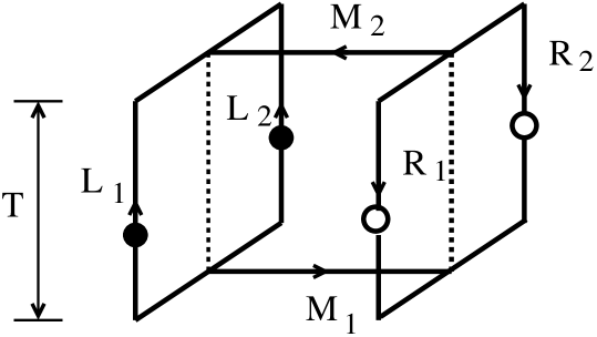
Figure 1: Wilson loop operator used by [2] and [3] to calculate the static potential of a tetraquark system.

This Wilson Loop has the quantum numbers of colour singlet system where the two quarks form an antitriplet and the two antiquarks form a triplet.

This lattice studies, indicate that the static potential of the two-quark and two-antiquark system is a generalized flip-flop potential:

$$V_{FF}=\min(V_{T},V_{M_{1}M_{2}},V_{M_{3}M_{4}})$$ (3)

where $V_{M_{1}M_{2}}$ and $V_{M_{3}M_{4}}$ are the two possible two-meson potentials, given by the sum of two independent intra-meson potentials $V_{M_{1}M_{2}}=V_{M_{1}}+M_{M_{2}}$, and $V_{T}$ is the tetraquark potential which corresponds to the sector where the four particles are confined, linked by a single fundamental string. It is given by

$$V_{T}=C+\alpha\sum_{i<j}\frac{\lambda_{i}}{2}\cdot\frac{\lambda_{j}}{2}+\sigma L_{min}\,,$$ (4)

where $L_{m}in$ is the minimal distance linking the four particles, which corresponds to the string configuration displayed on fig. 2.

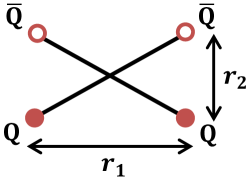
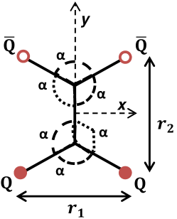
Figure 2: Here we can see the shape of the minimal string which links the four particles in the tetraquark. Note that when the diquark and the diantiquark are close the five segment structure collapses into a four segment one.

For the special case where the four particles form as rectangle as in fig. 2, $L_{min}$ is given by $L_{min}=\sqrt{3}r_{1}+r_{2}$ for $r_{2}>\frac{r_{1}}{\sqrt{3}}$ [6, 7]. If we neglect the Coulomb part of $V_{FF}$, we could estimate that the tetraquark sector becomes the ground state when $r_{2}\gtrsim\sqrt{3}r_{1}$.

3 Tetraquark Fields

The fields in the tetraquark system can be calculated by using the correlation of plaquettes and Wilson Loops. The Squared chromoelectric and chromomagnetic fields, are computed by

$$\langle E_{i}^{2}\rangle = \langle P_{0i}\rangle-\frac{\langle WP_{0i}\rangle}{\langle W\rangle}$$ (5)

$$\langle B_{i}^{2}\rangle = \frac{\langle WP_{jk}\rangle}{\langle W\rangle}-\langle P_{jk}\rangle$$

where the index $i$ complments $j$ and $k$. $P_{\mu\nu}$ is $P_{\mu\nu}=1-\frac{1}{3}\mbox{Tr}[U_{\mu}(\mathbf{s})U_{\nu}(\mathbf{s}+\hat{\nu})U_{\mu}^{\dagger}(\mathbf{s}+\hat{\nu})U_{\nu}^{\dagger}(\mathbf{s})]$.

The Lagrangian and energy densities are given by

$$\langle\mathcal{L}\rangle = \frac{1}{2}\langle E^{2}-B^{2}\rangle$$ (6)

$$\langle\mathcal{H}\rangle = \frac{1}{2}\langle E^{2}+B^{2}\rangle\,.$$

Now, we will present results for the chromo-fields for the tetraquark system for the simple case where the four particles form a rectangles, as in fig. 2.

This results, and the one of the following chapters were obtained using quenched lattice QCD configurations with dimension $24^{3}\times 48$ and $\beta=6.2$. They where used in GPUs by using a combination of Cabbibo-Marinari, pseudo heat-bath and over-relaxation algorithms [8]. APE smearing [9] and Hypercubic blocking [10] were used to improve the signal to noise ratio.

The results for the lagrangian density are given on fig. 3 for fixed $r_{2}=14$.

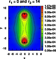
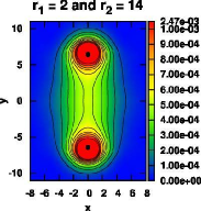
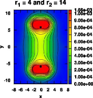
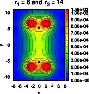
Figure 3: Plot of the lagrangian density for different values of $r_{1}$ with $r_{2}=14$.

As we can see the in the leftmost fig. $r_{1}=0$, in which case the system the system is collapsed in to a meson. Then we can see left to right, with the increase of $r_{1}$, the confining string acquires a shape similar with the one on fig. 2 for $r_{2}>\frac{r_{1}}{\sqrt{3}}$, in agreement with the result obtained for the static potential.

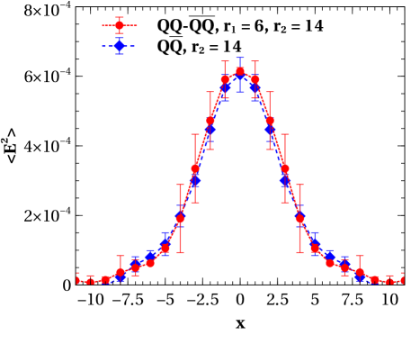
Figure 4: Comparision between the squared chromoelectric field in the quark-antiquark flux tube core (in the meson) and the diquark-antidiquark flux tube core (in the tetraquark).

In fig. 4 it is compared the squared chromoelectric fields $\langle\mathbf{E}^{2}\rangle$ in the flux tube centre of the meson and in the centre of the diquark-diantiquark flux tube in the tetraquark. As can be seen both the flux-tubes have a similar behaviour, which confirms that the string which is present in this system is a fundamental one, again in agreement with the results for the static potential.

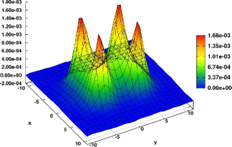
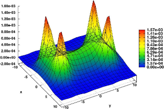
Figure 5: Lagrangian density in the flux tube for $r_{1}=r_{2}=8$ and $r_{1}=8,r_{2}=14$.

However, as can be seen in fig. 5 this agreement disappears for $r_{2}<\sqrt{3}r_{1}$ — the region where the ground state of the system is a two meson state and not the tetraquark state. As can be seen there, for $r_{1}=8$ and $r_{2}=14$ (tetraquark region), we obtained the expected ground state. However for $r_{1}=r_{2}=8$ (meson-meson region) we still see a string linking the four particles as in the tetraquark state, but we should see, to be in agreement with the generalized flip-flop model supported by the results obtained for the static potential, two strings corresponding to the two mesons. We think that this disagreement is due to the low overlap of the used operator with the ground state, and also to the small temporal extensions used in the Wilson Loop. To obtain the true ground state of the system in this region and also the first excited state we used a variational method.

4 Variational Method for the $QQ\bar{Q}\bar{Q}$ system

Now we will improve this method in order to obtain the true ground state of the system and also to obtain the first excited state. To achieve this, we note that the Wilson Loop operator could be written as a correlation of a certain operator at different times $W(t)=\langle\hat{\mathcal{O}}(t)\hat{\mathcal{O}}^{\dagger}(0)\rangle$. This could be generalized by considering instead a base of operators $\hat{\mathcal{O}}_{i}$. So this way, our wilson loop becomes a matrix $W_{ij}=\langle\hat{\mathcal{O}_{i}}\hat{\mathcal{O}}^{\dagger}_{j}\rangle$. This could be used not only to improve the ground state overlap but also to obtain more energy levels of the system. These are given by solving the generalized eigensystem

$$\langle W_{ij}(t)\rangle c_{n}^{j}(t)=w_{n}\langle W_{ij}(0)\rangle c_{n}^{j}(t)$$ (7)

The fields can then be calculated by $\langle P\rangle_{n}=\frac{\langle W_{n}P\rangle}{\langle W_{n}\rangle}-\langle P\rangle$ with $W_{n}=c_{n}^{i}W_{ij}c_{n}^{j}$.

We will consider again the case where the four particles form a rectangles and also two different alignments of the $QQ\bar{Q}\bar{Q}$ system. A parallel one, where the two quarks are on the same side of the rectangle and an antiparallel one, where the quarks are on opposite corners of the rectangle (fig. 6).

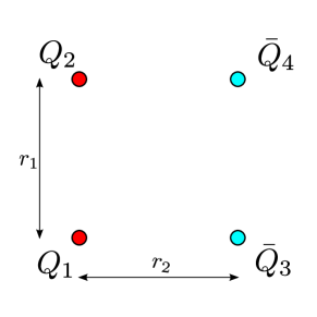
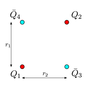
Figure 6: Left: Parallel alignment. Right: Antiparallel alignment.

For both cases we will use a base of two operators, similarly to what was made in [11]. In the parallel case the operators will be the tetraquark operator $\hat{\mathcal{O}}_{4Q}$, the correlation of which is the tetraquark Wilson Loop $W_{4Q}=\langle\hat{\mathcal{O}}_{4Q}(t)\hat{\mathcal{O}_{4Q}}(0)\rangle$, and a two meson operator. This gives a Wilson loop matrix where the diagonal elements are $W_{4Q}$ and the correlation of two wilson loops, while the off-diagonal elements correspond to the transition between the two states (see fig. 7

Figure 7: Elements of the Wilson loop matrix used for the parallel alignment.

For the antiparallel alignment, the operators used were the two meson-meson operators, giving the four matrix elements given on fig. 8.

Figure 8: Elements of the Wilson loop matrix used for the antiparallel alignment.

5 Results

Now, we present the results obtained for the parallel geometry.

In fig. 9 we can see the components of the chromoelectric and chromomagnetic fields for the ground state of the parallel alignment, with $r_{1}=6$ and $r_{2}=12$, while in fig. 10 the componentes are presented for the ground state of the antiparallel alignment with $r_{1}=6$ and $r_{2}=10$. The results indicate that what we have is essencialy a tetraquark in the first case and a two meson system in the second. Besides that we can see features that are common to flux-tubes in general [9] such as the dominance of the longitudinal chromoelectric field.

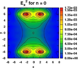
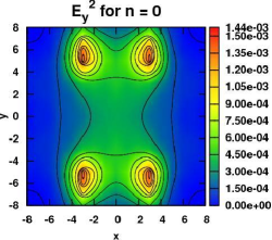
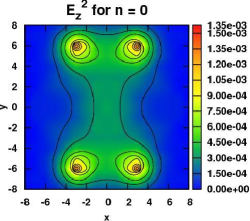
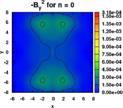
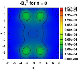
Figure 9: Components of the chromo-electromagnetic field, for the ground state of the parallel geometry with $r_{1}=6$ and $r_{2}=12$.

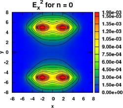
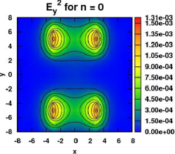
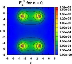
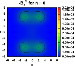
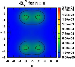
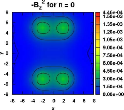
Figure 10: Components of the chromo-electromagnetic field, for the ground state of the anti-parallel geometry with $r_{1}=6$ and $r_{2}=10$.

In fig. 11 it is shown the evolution of the lagrangian density of the ground state of the parallel geometry, for fixed $r_{1}=6$. Here we can see the transition between the two meson state in the top-left picture ($r_{2}=6$) to the tetraquark state in the bottom right picture $r_{2}=12$. This is in agreement with the predictions of the generalized flip-flop potential contrary to the results we obtained using only the tetraquark operator $W_{4Q}$. The same evolution is presented in 12, but for the first excited state of the same configurations. This results are not so readily understandable.

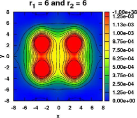
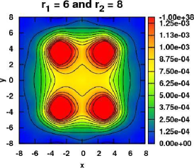
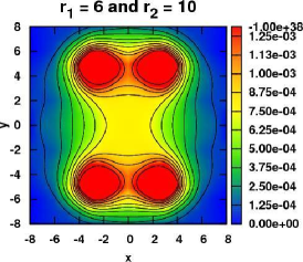
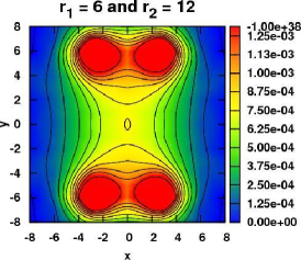
Figure 11: Lagrangian density for different values of $r_{1}$ and $r_{2}$ in the ground state of the parallel geometry.

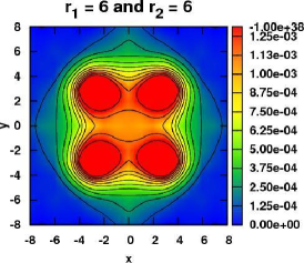
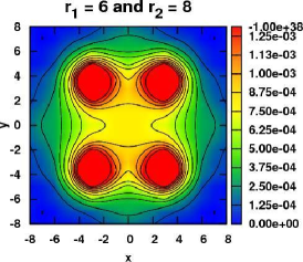
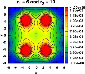
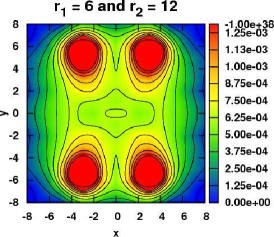
Figure 12: Lagrangian density for different values of $r_{1}$ and $r_{2}$ in the first excited state of the parallel geometry.

To better compare the ground and the first excited state we can look at fig. 13 in the $y=0$ axis.

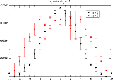
Figure 13: Comparasion of the action density in the center of flux tube in the parallel geometry for $r_{1}=6$ and $r_{2}=12$.

In fig. 14 we see the lagrangian density for the parallel alignment with varying $r_{1}$ and $r_{2}$. For $r_{1}=6$ and $r_{2}=10$ we can see the two mesons almost completely separatedly, while for $r_{1}=r_{2}$ we have a state when all the four particles are linked. We only show pictures for $r_{2}\geq r_{1}$. The case $r_{2}<r_{1}$ can be seen by rotating the pictures for $r_{2}>r_{1}$. This behaviour is again expected, as we obtain the separation in two mesons of the system when it correspond to the minimal string energy. The behaviour for $r_{1}=r_{2}$ is also expected, because neither of the two meson systems is preferred over the other.

The results for the first excited state are presented in fig. 15. As we can see there, the first excited state is different from a two meson state, with all the four particles being linked the flux-tube.

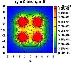
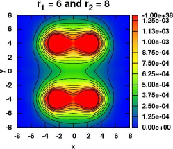
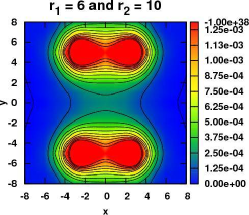
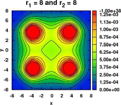
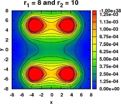
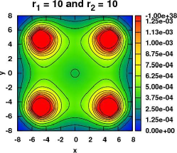
Figure 14: Lagrangian density for different values of $r_{1}$ and $r_{2}$ in the ground state of the anti-parallel geometry.

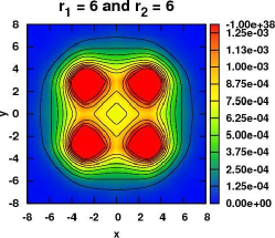
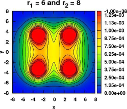
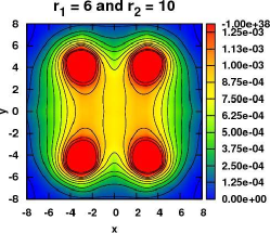
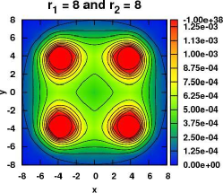
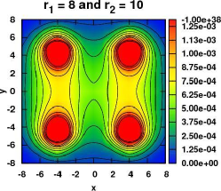
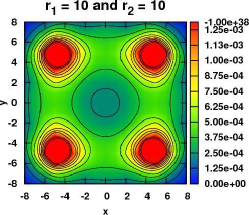
Figure 15: Lagrangian density for different values of $r_{1}$ and $r_{2}$ in the first excited state of the anti-parallel geometry.

Finally we compare the ground state and the first excited state in this geometry in fig. 16 for $y=0$, in the left, for $r_{1}=6$ and $r_{2}=10$, in the right for $r_{1}=r_{2}=10$. As can be seen, for the first case, the ground state flux-tube in this region is very small, because of the formation of two mesons.

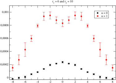
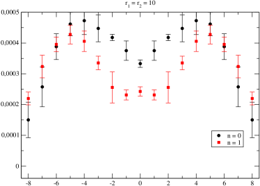
Figure 16: Comparasion of the action density in the center of flux tube in the anti-parallel geometry for two geometries.

6 Discussion

Our results for the fields of the two quarks and two antiquarks system agree with the results obtained for the static potential, therefore supporting a string picture of confinement with flux-tube recombination. Besides this, we were also able to calculate the first excited state of this system. The low overlap between the tetraquark operator and the two meson ground state may indicate small width tetraquark resonances. We are also studying the fields of the pentaquarks and the static potentials of this system.

This work was partly funded by the FCT contracts, PTDC/FIS/100968/2008, CERN/FP/109327/2009 and CERN/FP/116383/2010. Nuno Cardoso is also supported by FCT under the contract SFRH/BD/44416/2008 and Marco Cardoso is supported under contract SFRH/BPD/73140/2010 by the same institution.

References

- [1] R. L. Jaffe, “Multi-Quark Hadrons. 1. The Phenomenology of (2 Quark 2 anti-Quark) Mesons,” Phys. Rev., vol. D15, p. 267, 1977.
- [2] C. Alexandrou and G. Koutsou, “The static tetraquark and pentaquark potentials,” Phys. Rev., vol. D71, p. 014504, 2005.
- [3] F. Okiharu, H. Suganuma, and T. T. Takahashi, “The tetraquark potential and flip-flop in SU(3) lattice QCD,” Phys. Rev., vol. D72, p. 014505, 2005.
- [4] M. Oka, “HADRON HADRON INTERACTION IN THE STRING FLIPFLOP MODEL OF QUARK CONFINEMENT WITH COLOR, SPIN AND FLAVOR DEGREES OF FREEDOM. 1. MESON MESON INTERACTION,” Phys.Rev., vol. D31, pp. 2274–2287, 1985.
- [5] M. Oka and C. Horowitz, “HADRON HADRON INTERACTION IN THE STRING FLIPFLOP MODEL OF QUARK CONFINEMENT WITH COLOR, SPIN AND FLAVOR DEGREES OF FREEDOM. 2. NUCLEON NUCLEON INTERACTION,” Phys.Rev., vol. D31, pp. 2773–2779, 1985.
- [6] P. Bicudo and M. Cardoso, “Decays of tetraquark resonances in a two-variable approximation to the triple flip-flop potential,” Phys.Rev., vol. D83, p. 094010, 2011.
- [7] P. Bicudo and M. Cardoso, “Iterative method to compute the Fermat points and Fermat distances of multiquarks,” Phys. Lett., vol. B674, pp. 98–102, 2009.
- [8] 2011. the CUDA codes are available at Portuguese Lattice QCD collaboration, http://nemea.ist.utl.pt/~ptqcd.
- [9] M. Cardoso, N. Cardoso, and P. Bicudo, “Lattice QCD computation of the colour fields for the static hybrid quark-gluon-antiquark system, and microscopic study of the Casimir scaling,” Phys. Rev., vol. D81, p. 034504, 2010.
- [10] A. Hasenfratz and F. Knechtli, “Flavor symmetry and the static potential with hypercubic blocking,” Phys. Rev. D, vol. 64-3, p. 034504, 2001.
- [11] V. Bornyakov, P. Boyko, M. Chernodub, and M. Polikarpov, “Interactions of confining strings in SU(3) gluodynamics,” 2005.