Finite size scaling in minimal walking technicolor

Abstract

We compare observables to the finite size scaling hypothesis in SU(2) lattice gauge theory with two Dirac fermions in the adjoint representation. The fits that we obtain yield an estimate of the anomalous mass dimension that is consistent with four loop perturbation theory: $\gamma=0.51\pm 0.16$, with the error due to systematic uncertainties in the finite size scaling analysis. The result is somewhat larger than one Schrödinger functional study (by 1.3$\sigma$) but consistent with another.

I Introduction

In technicolor models, the Higgs mechanism occurs through condensation of new fermions that are subject to a gauge interaction that is strong at the TeV scale Susskind (1979); Weinberg (1979). Walking technicolor is a version of this theory that can suppress flavor-changing neutral currents by raising the extended technicolor scale, while still having phenomenologically acceptable Standard Model fermion masses, due to condensate enhancement Holdom (1981, 1985); Yamawaki et al. (1986); M. Bando, K. Matumoto, and K. Yamawaki (1986); Appelquist et al. (1986); Appelquist and Wijewardhana (1987a, b). Higher representations of the gauge group are believed to avoid problems with the S-parameter, i.e. electroweak precision constraints Eichten and Lane (1980); Lane and Eichten (1989). All of this has motivated the study of Minimal Walking Technicolor (MWTC) Sannino and Tuominen (2005), which is SU(2) gauge theory with two Dirac fermions in the adjoint (triplet) representation.

In order to study technicolor proposals nonperturbatively and from first principles, several groups have been using the techniques of lattice gauge theory; see the review Del Debbio (2010) and references therein. One of the key questions is whether the theory “walks” (very slow running of the coupling) or is attracted to an infrared fixed point (IRFP). An important quantity that can be computed in the process of answering this question is the anomalous mass dimension $\gamma$, which needs to satify $\gamma\approx 1$ in order for the standard walking technicolor picture to succeed. (Alternatives such as “ideal walking” are now being investigated as improvements over the standard picture Fukano and Sannino (2010).) One of the ways in which the lattice community has computed $\gamma$ is through the Schrödinger functional method. It was employed for SU(3) gauge group with sextet fermions in Shamir et al. (2008) and for MWTC in Bursa et al. (2010); DeGrand et al. (2011). Analysis of the distribution of eigenvalues of the Dirac operator has also been used Fodor et al. (2008); DeGrand (2009); Del Debbio and Zwicky (2010).

An alternative approach is to compare observables computed in lattice gauge theory (e.g., meson masses, the “pion” decay constant) to the finite size scaling (FSS) hypothesis. If the theory is indeed driven to an IRFP, then the data on observables should fit the FSS hypothesis. Previous studies of FSS in lattice technicolor include DeGrand (2009); Del Debbio et al. (2010a, b); DeGrand (2011). Fits to the conformal hypothesis that assume a specific form of the FSS function include Fodor et al. (2011); Appelquist et al. (2011), where the infinite volume hyperscaling relation is imposed. More general forms of the FSS function have also been considered recently by the authors of Fodor et al. (2011), with the result that for these forms the resulting conformal hypothesis for SU(3) gauge group and 12 fundamental flavors has a low degree of confidence in fitting the data Kuti . By contrast, DeGrand (2011) advocates an approach that does not impose a specific form on the FSS function; this is one of the FSS methods used in the earlier work DeGrand (2009). In this letter, we apply this method to the case of MWTC in order to extract an estimate of $\gamma$ under the assumption that an IRFP exists.

II Finite size scaling

In the scaling regime, the correlation length will have an asymptotic behavior dependent on the fermion mass $m$ with exponent $y_{m}$:

$$\xi\sim m^{-1/y_{m}}$$ (1)

This exponent is related to the anomalous mass dimension evaluated at the IRFP:

$$y_{m}=1+\gamma(g_{*})$$ (2)

It is a general consequence of the renormalization group equations that the correlation length $\xi_{L}$ at finite size $L$ is given by a scaling function of the infinite volume correlation length $\xi$ relative to $L$:

$$\xi_{L}/L=F(\xi/L)$$ (3)

Thus we obtain the FSS formula in terms of fermion mass:

$$\xi_{L}/L=f(mL^{y_{m}})$$ (4)

Corrections to scaling will be an important consideration for us. This translates into a correction that is appreciable for small $L$, with an exponent $\omega$:

$$\xi_{L}/L=f(mL^{y_{m}})+L^{-\omega}g(mL^{y_{m}})$$ (5)

This form has also been considered in Kuti ; there it was pointed out that fitting data to such a hypothesis would require an extensive and highly accurate study. For us the main use of this equation is just that the scaling violations are largest for the smallest values of $L$. We use this as an interpretation of data on small lattices that does not fall on a scaling curve. Our present study is not extensive enough to fit to this more general form and extract $\omega$. Below, we will consider $\xi_{L}=1/M$ or $1/f_{\pi}$, where $M$ is a meson mass.

III Fitting method

The method described here seeks to optimize $y_{m}$ such that all the data falls on a scaling curve. It is due to Bhattacharjee and Seno (2001) and was used in DeGrand (2009, 2011). For each $L$ we have a data set $p$. We use this to obtain a fit $f_{p}$. The types of fit functions that we consider will be described below. We then use this fit function on the other values of $L$, which we label as $L_{j}$.

We minimize the following function with respect to $y_{m}$.

$$P(y_{m})=\frac{1}{N_{\text{over}}}\sum_{p}\sum_{j\not=p}\sum_{i,\text{over}}\left(\frac{\xi_{L}(m_{i,j})}{L_{j}}-f_{p}(L_{j}^{y_{m}}m_{i,j})\right)^{2}$$ (6)

Here $i$ labels the different partially conserved axial current (PCAC) mass values for a given $L_{j}$. The effect of this is to find a $y_{m}$ such that $f_{p}$ for the other values $L_{j},m_{i,j}$ is as close as possible to the curve obtained from fitting $L_{p},m_{i,p}$. This is summed over all possibilities $p$. Also, “over” indicates that only $i$ are used such that $m_{i,j}L_{j}^{y_{m}}$ falls within the range of values of $m_{i,p}L_{p}^{y_{m}}$, so that the comparison is to an interpolation of the $m_{i,p}L_{p}^{y_{m}}$ data, rather than an extrapolation. Unweighted fits were used so that the approximation to the scaling curve would pass through data at small $x=mL^{y_{m}}$, where absolute (statistical) errors are largest. (Using a weighted fit reduces our conclusion for $\gamma$ by 4%.)

Type	$f(x)$
Quadratic	$c_{0}+c_{1}x+c_{2}x^{2}$
Log quadratic	$c_{0}+c_{1}\ln x+c_{2}(\ln x)^{2}$
Piece-wise log-linear	Straight lines connecting data

Table 1: Interpolating functions that we use to fit data for a fixed $L_{p}$. In the last case, the straight lines interpolating between data are on a semi-log plot.

For the fitting function we have considered the possibilities listed in Table 1. In the case of the quadratic we follow one of the methods of DeGrand (2009, 2011). The log quadratic fit was motivated by the behavior of the data when $\xi_{L}/L$ is plotted versus $\ln(mL^{y_{m}})$, which is close to a parabola. The piece-wise log-linear form was used as a third choice that trivially passes through the data, giving a reasonable interpolation.

IV Results

We have used four observables: the “pion” mass $m_{\pi}$, the “rho” mass $m_{\rho}$, the “$a_{1}$” mass $m_{a_{1}}$, and the “pion” decay constant $f_{\pi}$. These are all obtained from standard correlation functions using point sources and sinks. We fit the correlation functions with a single exponential, allowing the first time $t_{\text{first}}$ in the fit to be large enough for the excited state contributions to be negligible. This is determined by looking at the mass of the meson as a function of $t_{\text{first}}$ and extracting the value on the plateau. Five values of bare masses $m_{0}a=-1.0,-1.1,-1.165,-1.175,-1.18$ on lattices of size $L/a=10,12,16,20,24$ were simulated, all at $\beta=2.25$. These are the same configurations as were generated in Giedt and Weinberg (2011), and the values of the PCAC mass and details on the simulations are given there. Also note that the size of the temporal direction is $T=2L$.

Figure 1: Collapse of $\pi$ data for $y_{m}=1.46$. Here and in the other figures, $x=mL^{y_{m}}$.

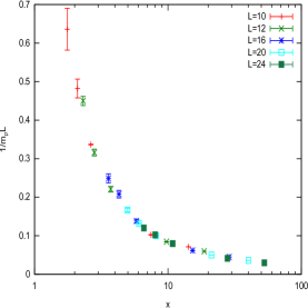
Figure 2: Collapse of $\rho$ data for $y_{m}=1.50$.

Using these results, and performing the minimization described in the previous section, we obtain values for $y_{m}$. In the case of $m_{a_{1}}$ and $f_{\pi}$, the quantity $\xi_{L}/L$ is small, and scaling violations [cf. Eq. (5)] can compete with the scaling function for small lattices. For this reason we exclude the small lattices $L/a=10,12$ for these channels. The results for $y_{m}$ are summarized in Table 2. It can be seen that each of the channels, and each of the fitting methods are consistent with each other within errors. The approximate collapse of data is shown in Figs. 1-4; it can be seen in Figs. 3 and 4 that the excluded small lattice data does not fall on the scaling curve. We interpret this as being due to scaling violations, though a thorough study extracting $\omega$ would be required to demonstrate this. Another interpretation is that the theory does not have an IRFP, and so the FSS fails for some channels. It is also possible that we are seeing the effect of $\beta=2.25$ not being close enough to the fixed point coupling. However we view the collapse seen in Figs. 1 and 2 as favoring our scaling violation interpretation.

Observable	Quadratic	Log Quad	PWL	Combined
$m_{\pi}$	1.67(93)	1.26(54)	1.51(33)	1.46(27)
$m_{\rho}$	1.67(88)	1.37(39)	1.56(31)	1.50(23)
$m_{a_{1}}$	1.40(52)	1.42(27)	1.41(22)	1.41(16)
$f_{\pi}$	1.65(22)	1.49(54)	1.60(29)	1.62(17)

Table 2: The scaling exponent $y_{m}=1+\gamma$ for the various observables and methods of interpolation. In parentheses, jackknife error is shown, obtained from eliminating one $m_{i,j}$ in all possible ways, in the minimization of (6). Because we use a large number of configurations, ${{\cal O}(10^{3})}$, statistical error is negligible by comparison.

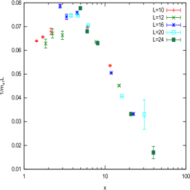
Figure 3: The $a_{1}$ data for $y_{m}=1.41$. The $L=10,12$ data do not fall on the curve, which we interpret as large scaling violations. These points were excluded from the fit.

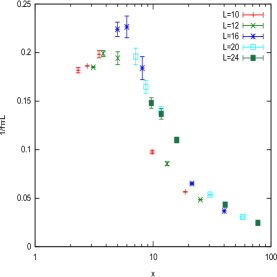
Figure 4: The $f_{\pi}$ data for $y_{m}=1.62$. The $L=10,12$ data do not fall on the curve, which we interpret as large scaling violations. These points were excluded from the fit.

We average the twelve values of $y_{m}$ for the four channels and three fitting methods, weighted by the jackknife errors, to obtain $\overline{\gamma}=0.51$. The combined jackknife error from the twelve fits is 0.097, and the standard deviation of the twelve fits is 0.128. We regard these as two sources of systematic error and combine them in quadrature to obtain a final estimate of

$$\gamma=0.51\pm 0.16$$ (7)

In Table 3, we compare this estimate with results from other groups using a variety of methods. Our result is consistent with one of those obtained using the Schrödinger functional Bursa et al. (2010), perturbation theory, Monte Carlo renormalization group and the all-orders hypothesis of Pica and Sannino (2011a). We obtain a value significantly larger than the one obtained in the FSS studies Del Debbio et al. (2010a, b) (1.8$\sigma$ difference) and somewhat larger than the Schrödinger functional study DeGrand et al. (2011) (1.3$\sigma$ difference).

Method	$\gamma$
SF Bursa et al. (2010)	$0.05<\gamma<0.56$
SF DeGrand et al. (2011)	$0.31\pm 0.06$
Perturbative 4-loop Pica and Sannino (2011b)	$0.500$
Schwinger-Dyson Ryttov and Shrock (2011)	$0.653$
All-orders hypothesis Pica and Sannino (2011a)	$0.46$
MCRG Catterall et al. (2011)	$-0.6<\gamma<0.6$
FSS Del Debbio et al. (2010a)	$0.05<\gamma<0.20$
FSS Del Debbio et al. (2010b)	$0.22\pm 0.06$
FSS (here)	$0.51\pm 0.16$

Table 3: Summary of all MWTC results for the anomalous mass dimension. SF is Schrödinger functional and MCRG is Monte Carlo renormalization group. The perturbative result $\gamma=0.500$ was also given in the later, corrected version of Ryttov and Shrock (2011), and relied on invariants calculated in Mojaza et al. (2010).

V Conclusions

We have applied the FSS approach of DeGrand (2011) (one of the approaches in DeGrand (2009)) to MWTC and find values of the critical exponent that are in agreement with perturbative results, but somewhat higher than the Schrödinger functional result with the smallest estimate of error DeGrand et al. (2011), by 1.3$\sigma$. While there are significant systematic uncertainties, which we interpret as being due to scaling violations on small volumes, the value of $\gamma$ is too small for phenomenological models of condensate enhancement, which requires $\gamma\approx 1$. The complimentary information obtained by the present method suggests that it be applied in other gauge theories of interest for conformal or near-conformal dynamics. Indeed we expect it to work in any case for which the gauge coupling runs very slowly, so that fixed point behavior is well approximated on the scales probed by the study that is performed. Unfortunately, as explained in DeGrand (2011), a reasonable fit to the FSS assumption does not rule in or out the existence of an IRFP, since all that is required is a very slow running.

We have highlighted some of the systematic uncertainties of the method, and have illustrated how working on small volumes hampers the effort to obtain an accurate $y_{m}$. Future work includes simulations on larger volumes so that $y_{m}$ can be obtained with greater certainty. Also, an improved lattice action should reduce the size of the scaling violations, and we are currently working in that direction for MWTC and other theories.

References

- Susskind (1979) L. Susskind, Phys. Rev. D20, 2619 (1979).
- Weinberg (1979) S. Weinberg, Phys. Rev. D19, 1277 (1979).
- Holdom (1981) B. Holdom, Phys. Rev. D24, 1441 (1981).
- Holdom (1985) B. Holdom, Phys. Lett. B150, 301 (1985).
- Yamawaki et al. (1986) K. Yamawaki, M. Bando, and K.-i. Matumoto, Phys. Rev. Lett. 56, 1335 (1986).
- M. Bando, K. Matumoto, and K. Yamawaki (1986) M. Bando, K. Matumoto, and K. Yamawaki, Phys. Lett. B178, 308 (1986).
- Appelquist et al. (1986) T. W. Appelquist, D. Karabali, and L. C. R. Wijewardhana, Phys. Rev. Lett. 57, 957 (1986).
- Appelquist and Wijewardhana (1987a) T. Appelquist and L. C. R. Wijewardhana, Phys. Rev. D35, 774 (1987a).
- Appelquist and Wijewardhana (1987b) T. Appelquist and L. C. R. Wijewardhana, Phys. Rev. D36, 568 (1987b).
- Eichten and Lane (1980) E. Eichten and K. D. Lane, Phys. Lett. B90, 125 (1980).
- Lane and Eichten (1989) K. D. Lane and E. Eichten, Phys. Lett. B222, 274 (1989).
- Sannino and Tuominen (2005) F. Sannino and K. Tuominen, Phys. Rev. D71, 051901 (2005), arXiv:hep-ph/0405209 .
- Del Debbio (2010) L. Del Debbio, PoS LATTICE2010, 004 (2010).
- Fukano and Sannino (2010) H. S. Fukano and F. Sannino, Phys.Rev. D82, 035021 (2010), arXiv:1005.3340 [hep-ph] .
- Shamir et al. (2008) Y. Shamir, B. Svetitsky, and T. DeGrand, Phys. Rev. D78, 031502 (2008), arXiv:0803.1707 [hep-lat] .
- Bursa et al. (2010) F. Bursa, L. Del Debbio, L. Keegan, C. Pica, and T. Pickup, Phys.Rev. D81, 014505 (2010), arXiv:0910.4535 [hep-ph] .
- DeGrand et al. (2011) T. DeGrand, Y. Shamir, and B. Svetitsky, (2011), arXiv:1102.2843 [hep-lat] .
- Fodor et al. (2008) Z. Fodor, K. Holland, J. Kuti, D. Nogradi, and C. Schroeder, PoS LATTICE2008, 058 (2008), arXiv:0809.4888 [hep-lat] .
- DeGrand (2009) T. DeGrand, Phys.Rev. D80, 114507 (2009), arXiv:0910.3072 [hep-lat] .
- Del Debbio and Zwicky (2010) L. Del Debbio and R. Zwicky, Phys.Rev. D82, 014502 (2010), arXiv:1005.2371 [hep-ph] .
- Del Debbio et al. (2010a) L. Del Debbio, B. Lucini, A. Patella, C. Pica, and A. Rago, Phys.Rev. D82, 014509 (2010a), arXiv:1004.3197 [hep-lat] .
- Del Debbio et al. (2010b) L. Del Debbio, B. Lucini, A. Patella, C. Pica, and A. Rago, Phys.Rev. D82, 014510 (2010b), arXiv:1004.3206 [hep-lat] .
- DeGrand (2011) T. DeGrand, Phys.Rev. D84, 116901 (2011), arXiv:1109.1237 [hep-lat] .
- Fodor et al. (2011) Z. Fodor, K. Holland, J. Kuti, D. Nogradi, C. Schroeder, et al., Phys.Lett. B703, 348 (2011), arXiv:1104.3124 [hep-lat] .
- Appelquist et al. (2011) T. Appelquist, G. Fleming, M. Lin, E. Neil, and D. Schaich, Phys.Rev. D84, 054501 (2011), arXiv:1106.2148 [hep-lat] .
- (26) J. Kuti, Talk given at Lattice 2011, July 10-16, 2011, Squaw Valley, USA.
- Bhattacharjee and Seno (2001) S. M. Bhattacharjee and F. Seno, Jour. of Phys. A34, 6375 (2001).
- Giedt and Weinberg (2011) J. Giedt and E. Weinberg, Phys.Rev. D84, 074501 (2011), arXiv:1105.0607 [hep-lat] .
- Pica and Sannino (2011a) C. Pica and F. Sannino, Phys.Rev. D83, 116001 (2011a), arXiv:1011.3832 [hep-ph] .
- Pica and Sannino (2011b) C. Pica and F. Sannino, Phys.Rev. D83, 035013 (2011b), arXiv:1011.5917 [hep-ph] .
- Ryttov and Shrock (2011) T. A. Ryttov and R. Shrock, Phys.Rev. D83, 056011 (2011), arXiv:1011.4542 [hep-ph] .
- Catterall et al. (2011) S. Catterall, L. Del Debbio, J. Giedt, and L. Keegan, (2011), arXiv:1108.3794 [hep-ph] .
- Mojaza et al. (2010) M. Mojaza, C. Pica, and F. Sannino, Phys.Rev. D82, 116009 (2010), arXiv:1010.4798 [hep-ph] .