Detailed compositional analysis of the heavily polluted DBZ white dwarf SDSS J073842.56+183509.06: A window on planet formation?

Abstract

We present a new model atmosphere analysis of the most metal contaminated white dwarf known, the DBZ SDSS J073842.56+183509.06. Using new high resolution spectroscopic observations taken with Keck and Magellan, we determine precise atmospheric parameters and measure abundances of 14 elements heavier than helium. We also report new Spitzer mid-infrared photometric data that are used to better constrain the properties of the debris disk orbiting this star. Our detailed analysis, which combines data taken from 7 different observational facilities (GALEX, Gemini, Keck, Magellan, MMT, SDSS and Spitzer) clearly demonstrate that J0738+1835 is accreting large amounts of rocky terrestrial-like material that has been tidally disrupted into a debris disk. We estimate that the body responsible for the photospheric metal contamination was at least as large Ceres, but was much drier, with less than 1% of the mass contained in the form of water ice, indicating that it formed interior to the snow line around its parent star. We also find a correlation between the abundances (relative to Mg and bulk Earth) and the condensation temperature; refractory species are clearly depleted while the more volatile elements are possibly enhanced. This could be the signature of a body that formed in a lower temperature environment than where Earth formed. Alternatively, we could be witnessing the remains of a differentiated body that lost a large part of its outer layers.

1. INTRODUCTION

The heavy elements observed in the spectra of otherwise pure hydrogen or helium atmosphere white dwarfs represent handy fingerprints of asteroids/rocky planets that survived the late phases of stellar evolution (Zuckerman et al., 2007; Klein et al., 2010, 2011; Dufour et al., 2010). There is growing evidence that perhaps all metal polluted white dwarfs of spectral type DZ, DBZ and DAZ have acquired their heavy material from an orbiting debris disk reservoir whose origin is explained by the tidal disruption of one or many large rocky bodies that ventured too close to the star (Debes & Sigurdsson, 2002; Jura, 2003, 2006; Jura et al., 2007; Jura, 2008; Farihi et al., 2010a, b; Melis et al., 2010). Such disks, which are easily detectable at infrared wavelengths, are now discovered with an accelerating pace with more than 20 cases uncovered in the last 6 years alone (see Farihi et al., 2009; Farihi, 2011; Kilic et al., 2011, and references therein).

Meanwhile, high resolution observations in the optical also revealed the presence of weak calcium lines in many white dwarfs, suggesting that at least 25% of their progenitors possessed orbiting planetary bodies with masses often comparable to that of the largest solar system asteroids (Zuckerman et al., 2003, 2010). Unfortunately, the majority of the known metal polluted white dwarfs only show one or two heavy elements in the optical, hardly enough to make detailed planetary composition inquiries (Dufour et al., 2007). In a few extreme cases, however, a handful of elements are observed, opening a unique window for studying rocky exoplanet compositions. The first investigations, those of GD 362 and GD 40 (Zuckerman et al., 2007; Klein et al., 2010) revealed striking similarity between the accreted bodies and bulk Earth material, providing the first comprehensive measurements of the bulk elemental composition of ancient planetary systems. Analysis of similar objects, based on Keck high resolution observations, quickly followed these pionering studies, bringing to 6 the number of metal polluted white dwarfs with more than 8 heavy elements detected in the optical (the previous two along with G241$-$6, NLTT 43806, PG 1225$-$079 and HS 2253+8023, Zuckerman et al., 2010, 2011; Klein et al., 2011).

Although the global abundance patterns found for these few objects were relatively well explained by the accretion of rocky planetary material similar to bulk Earth, closer looks reveal a wide range of compositional diversity from star to star (or, equivalently, planets to planets), especially for the most refractory elements. Interestingly, dynamical simulations such as those of Bond et al. (2010a, b) also predict a wide variety of chemical properties and structure compared to what is observed in the solar system. The most metal polluted white dwarfs could thus represent perfect testbeds to discriminate between various planet formation scenarios, allowing the first empirical verification of extrasolar terrestrial planet formation simulations. However, other processes such as post AGB thermal heating, collisions and wind stripping, could also play an important role in the final bulk composition that is measured at a white dwarf photosphere. Understanding the physical mechanisms responsible for the various observed elemental abundance patterns represents one of the biggest challenge of this relatively young field of research. As the sample of well studied metal contaminated white dwarfs increases, a more comprehensive picture should emerge, leading to a better understanding of how, both individually and statistically, these planetary systems form and evolve.

Recently, Dufour et al. (2010) discovered an extremely polluted DBZ white dwarf, SDSS J073842.56+183509.06 (hereafter J0738+1835) in the Sloan Digital Sky Survey. A preliminary analysis, based on medium resolution optical spectroscopy, revealed the presence of O, Mg, Si, Ca and Fe in record quantities. Given that Keck/HIRES spectroscopy of the heavily polluted white dwarf GD 362 revealed 15 different heavy elements (Zuckerman et al., 2007), three of which are detected in low resolution spectroscopy (Gianninas et al., 2004), we anticipated that higher resolution observations of J0738+1835 would reveal several additional elements not detected in Dufour et al. (2010)’s low resolution data.

This paper reports a detailed analysis of J0738+1835 based on new high resolution optical spectra taken at the Keck and Magellan telescopes. We also report new mid-infrared photometric data taken with Spitzer which, when combined with Gemini $JHK$ photometry, provides better constraints on the debris disk physical properties. In addition to the heavy elements already detected by Dufour et al. (2010), our new spectroscopic observations of J0738+1835 reveal the presence of 9 new elements (Na, Al, Sc, Ti, V, Cr, Mn, Co and Ni), for a total of 14 chemical species heavier than helium. This is the second highest number of heavy elements ever observed at a white dwarf photosphere (the champion, with 15 different metals, being GD 362; Zuckerman et al., 2007) thus making J0738+1835 a new and important member of the very select group of polluted white dwarfs with eight or more elements heavier than helium detected optically (Zuckerman et al., 2011).

In § 2, we describe the new observations. Our detailed analysis of the spectroscopic and photometric observations follows in § 3 while the results are discussed and summarized in § 4 and § 5.

2. OBSERVATIONS

Our detailed study of SDSS J0738+1835 uses data taken from 7 different observational facilities (GALEX, SDSS, Gemini, MMT, Keck, Magellan and Spitzer), with a strong emphasis on new Keck HIRES spectroscopy. Part of these data have already been presented in the preliminary analysis of Dufour et al. (2010) and are not discussed further here. Below we describe the new data.

2.1. Keck/HIRES

We used the High Resolution Echelle Spectrometer (HIRES, Vogt et al., 1994) on the Keck I 10m telescope (Mauna Kea Observatory) to obtain high resolution optical spectroscopy of J0738+1835 over 4 hours on UT 2011 March 23. We use the blue collimator and the 1.148$\arcsec$ slit with the cross disperser angle of 1.075, providing wavelength coverage from 3100 Å to 5990 Å with a resolving power of 37,000. The seeing started at 0.9” with an average around 1.1 $\arcsec$. We use the MAuna Kea Echelle Extraction (MAKEE) software for data analysis. We flat-field the exposures, optimally extract the spectra from the two dimensional image traced by the standard star Feige 34 observed on the same night, remove cosmic rays, and wavelength calibrate the spectra using Th-Ar lamps. MAKEE does not extract spectra in a few of the partially covered orders. We use the HIRES Redux package written by J. X. Prochaska to extract these missing orders from the MAKEE pipeline. The HIRES observations of J0738+1835 is thus composed of 58 short spectroscopic segments, typically 60 to 90 Å wide, with some wavelength overlap in adjacent orders. The overlapping parts have been co-added to slightly improve the signal-to-noise ratio.

2.2. Magellan/MagE Optical Spectroscopy

Moderate-resolution optical spectra of J0738+1835 were obtained on 2011 March 19 (UT) with the Magellan Echellette (MagE; Marshall et al., 2008), mounted on the 6.5m Landon Clay Telescope at Las Campanas Observatory. Conditions during the observations were clear with 0.6$\arcsec$ seeing. Two exposures of 1200 s each were obtained over an airmass range of 1.48–1.49 using the 0.7$\arcsec$ slit aligned with the parallactic angle; this setup provided 3200–10050 Å spectroscopy at a resolution $\approx$ 8000 (although only the red part longward of 6000 Å, where some important oxygen lines are present, is used in the present analysis since the Keck observations covers the rest with a better resolution and signal-to-noise ratio).

We also observed the spectrophotometric flux standard Hiltner 600 (Hamuy et al., 1994) on the same night for flux calibration. Th-Ar lamps were obtained after each source observation for wavelength calibration. Order tracing and pixel response were calibrated with internal Xe lamp flats and twilight sky flats, respectively, obtained at the beginning of the night. Data were reduced using the MASE reduction pipeline (Bochanski et al., 2009), following standard procedures for order tracing, flat field correction, vacuum wavelength calibration (including heliocentric correction), optimal source extraction, order stitching, and flux calibration.

2.3. MMT spectroscopy

We used the 6.5m MMT equipped with the Blue Channel spectrograph to obtain medium resolution spectroscopy of J0738+1835 over 109 minutes on UT 2010 March 19. We operate the spectrograph with the 832 line mm^-1 grating in second order, providing wavelength coverage from 3170 Å to 4100 Å and a spectral resolution of $\approx$ 1 Å. All spectra were obtained at the parallactic angle. We used He-Ne-Ar comparison lamp exposures and blue spectrophotometric standards (Massey et al., 1988) for wavelength and flux calibration, respectively. We reduce the data using standard IRAF routines.

2.4. Spitzer

We used the warm Spitzer equipped with the InfraRed Array Camera (IRAC, Fazio et al., 2004) to obtain mid-infrared photometry of J0738+1835 on UT 2010 December 1 as part of program 70023. We obtained 3.6 and 4.5 $\mu$m images with integration times of 100 seconds for nine dither positions. We use the IDL astrolib packages to perform aperture photometry on the individual corrected Basic Calibrated Data frames from the latest available pipeline reduction. We get similar results using 2 and 3 pixel apertures, but we quote the results using the smallest aperture since it has the smallest errors.

Following the IRAC calibration procedures, we correct for the location of the source in the array before averaging the fluxes of each of the dithered frames at each wavelength. We also correct the Channel 1 (3.6 $\mu$m) photometry for the pixel-phase-dependence. We estimate the photometric error bars from the observed scatter in the nine images corresponding to the dither positions. We add the 3% absolute calibration error in quadrature (Reach et al., 2005). Reach et al. (2009) demonstrate that the color corrections for dusty white dwarfs like G29-38 are small (0.4-0.5%) for channels 1 and 2. We ignore these corrections for J0738+1835.

The final observed flux and uncertainties at 3.6 $\mu$m and 4.5 $\mu$m are 81.1 $\pm$ 2.7 $\mu$Jy and 76.7 $\pm$ 2.7 $\mu$Jy respectively.

3. DETAILED ANALYSIS

3.1. Model Atmospheres and Fitting Technique

The model atmosphere and synthetic spectrum calculations are performed using the same code that was used in the first attempt to model J0738+1835 (Dufour et al., 2010) with the exception that we now use atomic data provided by the Vienna Atomic Line Database (VALD) instead of the Kurucz line list.

As a first step, we calculated a model structure using the same parameters ($T_{\rm eff}$, $\log g$ and abundances) as Dufour et al. (2010), including all the transitions (from 200 to 10,000 Å) present in our linelist. Using this thermodynamic structure, we next calculated several grids of synthetic spectra, one for each element of interest, keeping the abundance of all other elements fixed to their original values. For example, the Fe grid covers a range of abundance from log [n(Fe)/n(He)] = $-$4.0 to $-$6.0 in steps of 0.5 dex with the abundances of all other metals fixed to those previously determined. The various grids typically vary by log [n(Z)/n(He)] = $\pm$1.5 dex (in step of 0.5 dex) around the previously determined (or expected by assuming $\rm CI$ chondrites ratios from Lodders, 2003) abundance. These grids are then used to determine the different elemental abundances as follows.

Since the optical spectra for J0738+1835 are extremely crowded with several hundred lines, many of which overlap, it is not practical to fit each line individually using equivalent width measurements. Instead, we made short segments, typically 15 to 30 Angstrom wide, centered on each of the strongest absorption features observed in our dataset (i.e., those that are unambiguously detected and deeper than $\sim$10% of the continuum flux level). Then, each segment (a few hundreds) are fitted separately with the appropriate grids.

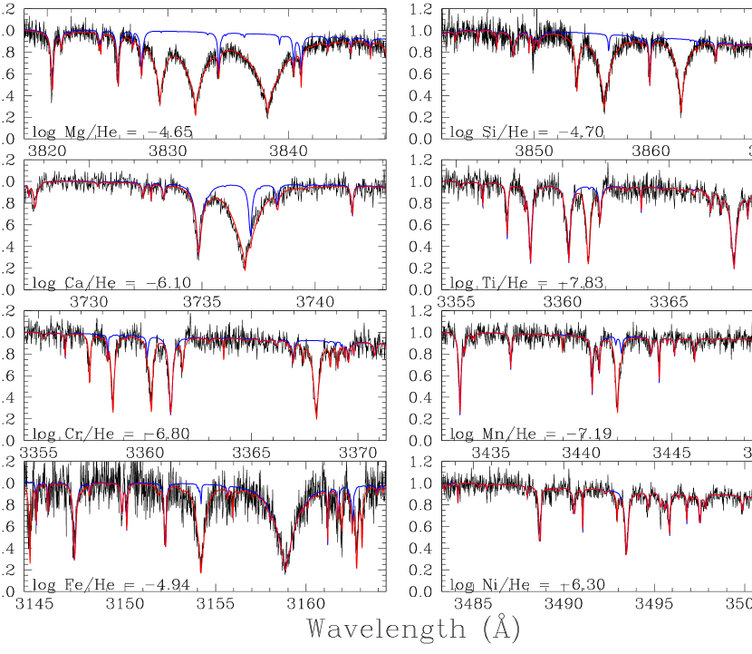
Figure 1.— Typical example of fits to small HIRES segments. Only one element at a time is fitted in each panel, all other elements being kept fixed to the value determined in the previous iteration (see text). The determined abundance of the element of interest, which is not the final abundance reported in Table 2, is indicated in the lower left corner of each panel. The red line is our best fit while the blue line is a synthetic spectrum where the element of interest has been removed to help localize the regions where the fitted lines contribute. The observations have been artificially shifted to air wavelengths in order to facilitate line identification using line lists.

Our fits are done by minimizing the value of the $\chi^{2}$ taken as the sum of the difference between the observed and model fluxes over the wavelength range of interest, all frequency points being given an equal weight. We consider the abundance, the solid angle and a linear term to account for the slope (the numerous HIRES orders are not flux calibrated) as free parameters. This method allows a very good determination of the local continuum and naturally takes into account the contribution of the absorption from other elements. It is thus particularly well suited for situations where it is difficult to precisely determine equivalent widths of individual lines, either because line blending is important or the signal-to-noise ratio is marginal. We show in Figure 1 typical examples of segment fits. In order to better visualize the fitted features, we plotted in blue a synthetic spectrum in which the element that is fitted has completely been removed. We note that in many cases, more than one line from a given fitted element can be found in a single segment. In these cases, the determined abundance of the segment is essentially a weighted average of the lines, more weight (more frequency points) being put on the strongest lines. We finally take as the measured abundance of an element the average over all the segments.

It must be noted, however, that these abundances were determined from synthetic spectra calculated with a structure corresponding to the Dufour et al. (2010) solution. The presence of new species, as well as the slightly different abundances that we now derive (and, to a smaller extent, the use of the VALD data), has a small impact on the thermodynamic structure of our model. Hence, in order to obtain a self-consistent solution, it is necessary to repeat the above mentioned procedure (i.e., recalculate all the grids and redo the fits) but, this time, starting from a model structure calculated with the newly determined set of abundances. We iterate until the input abundances in the model structure and the final measurements from our grids are in agreement.

However, even this solution can not be considered final since such an analysis is done for a fixed value of $T_{\rm eff}$ and $\log g$ (13,600 K and 8.5, respectively). These parameters were originally determined from fitting the HeI line profiles as well as simultaneously accommodating the MgI and MgII line strengths (see Dufour et al., 2010). As discussed in Klein et al. (2010, 2011), the absolute abundance of the various elements can vary significantly (up to 0.4 dex in some stars) with small variations of $T_{\rm eff}$and $\log g$. The relative composition of the polluting elements, however, are much less sensitive to the exact final parameters adopted and can thus be used as a high precision measurement of the accreted planets/planetesimals (see below). Nevertheless, we believe it is best to take full advantage of the opportunities provided by our dataset, and proceed in obtaining the best atmospheric parameters as possible by reevaluating the effective temperature, the surface gravity and the elemental abundances in a self consistent way.

We thus repeated the whole analysis as described above but, this time, starting with model structures calculated at effective temperatures of 13,300 and 13,900 K (corresponding to the estimated uncertainties of $\pm$300 K in Dufour et al., 2010). We then focus on elements for which lines from two different ionization state are present. In particular, we select a subsample of the strongest well isolated lines of Mg and Fe, the elements that show the largest number of lines from both the neutral and ionized state. In Figures 2 and 3, we plot the average abundance for each ion as a function of effective temperature, taking the standard deviation of the set of individual abundances as error bars. Clearly, a much better agreement between the two ionization states is obtained for a slightly higher effective temperature than first obtained by Dufour et al. (2010). A remarkable agreement between the various ion abundances is reached for an effective temperature of $\sim$ 13,950 K. This effective temperature estimate, which is determined solely from Mg and Fe lines, is completely independent of the uncertain treatment of van der Waals HeI line broadening.

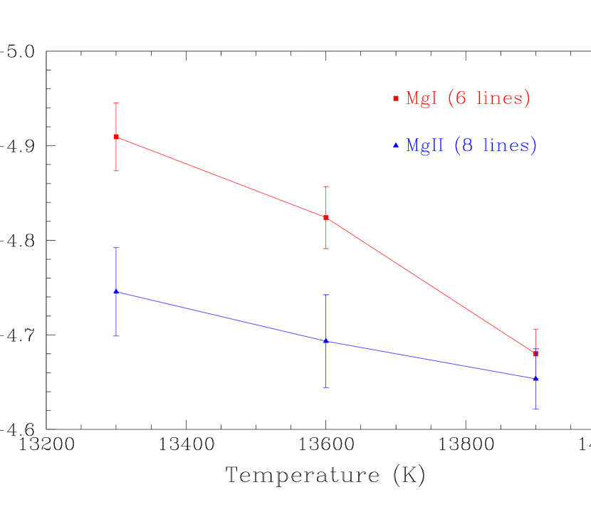
Figure 2.— Average abundances of magnesium lines as a function of effective temperature for two different ionization states. The error bars represent the standard deviation of the set of individual. A much better internal coherence is found for an effective temperature near 13,950 K.

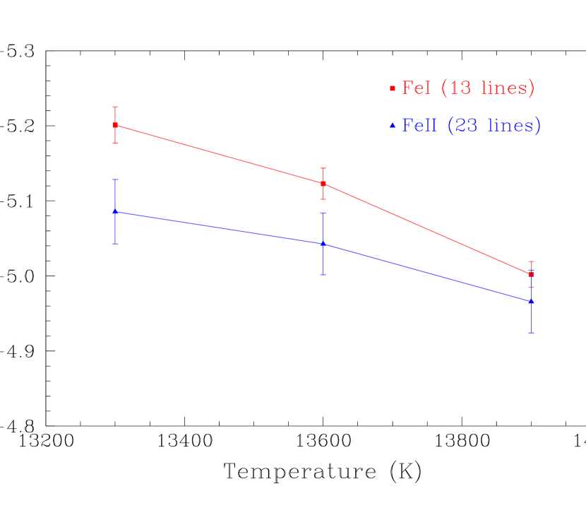
Figure 3.— Same as Figure 2, but for iron.

Next, we take this newly determined effective temperature and repeat again the above procedure but this time with surface gravities between $\log g$= 8.3 and 8.7. Our results, summarized in Figure 4 and 5, indicate that a surface gravity lower than $\log g$= 8.5 better reproduces the different ion abundances. A surface gravity of $\log g$$\sim$ 8.4 is preferred by the Mg lines while a slightly lower surface gravity is required for the Fe lines, although a value of $\log g$$\sim$8.4 is compatible with the error bars.

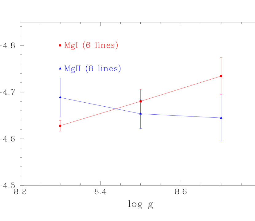
Figure 4.— Average abundances of magnesium lines as a function of surface gravity for two different ionization states. The error bars represent the standard deviation of the set of individual. A slightly lower surface gravity than $\log g$= 8.5 appears to be preferable.

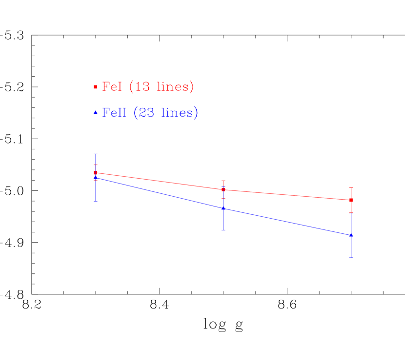
Figure 5.— Same as Figure 4, but for iron.

We thus adopt, as our final parameters, an effective temperature of 13,950 K and a surface gravity of $\log g$$\approx$ 8.4 with conservative uncertainties of $\pm$100 K and $\pm$0.2 dex respectively. These uncertainties are next properly propagated for the determination of errors on the cooling age, luminosity, mass, radius and distance of the star (obtained using the solid angle from $ugriz$ photometry). The evolutionary models used are similar to those described in Fontaine et al. (2001) but with C/O cores, and thickness of the helium and hydrogen layers of respectively q(He) = 10^-2 and q(H) = 10^-10, which are representative of helium-rich atmosphere white dwarfs. To evaluate the abundance uncertainties, we proceed in a similar manner to that described in Klein et al. (2010) and vary the model $T_{\rm eff}$  and $\log g$  by their uncertainties, one at a time, determine the average change in abundances for each parameter, and add them in quadrature to the standard deviation of the set of individual abundances. Our final parameters are presented in Table 1 and 2 while our best fit models are plotted over the spectroscopic data for the most interesting HIRES and MagE orders in Figures 6 to 12.

Table 1Stellar parameters adopted for SDSS J0738+1835

Parameter	Value
$T_{\rm eff}$(K)	13950 $\pm$ 100
$\log g$	8.4 $\pm$ 0.2
$M_{\rm WD}/M_{\odot}$	0.841 $\pm$ 0.131
$M_{\rm init}/M_{\odot}$	4.47 $\pm$0.36 a
$R/R_{\odot}$	0.00958 $\pm$ 0.0015
$\log L/L_{\odot}$	$-$2.50 $\pm$0.12
$D$	147 pc $\pm$23
Cooling Age	477 Myr $\pm$ 160
$\log(M_{\rm He}/M_{\star})$	$-$6.41 $+0.56$/$-0.28$

Table 2

Element	log $[n(Z)/n(He)]_{phot}$	$M_{\rm CVZ}/(10^{21}$g)	log $\tau_{set}$(yr)	$[n(Z)/n(Fe)]_{acc}$	$\dot{M}/(10^{8}g~{}s^{-1})$
1  H	-5.73 $\pm$ 0.17	0.310	$\infty$	…	…
8  O	-3.81 $\pm$ 0.19	407.86	5.244	9.52	740.2
11 Na	-6.36 $\pm$ 0.16	1.639	5.238	$2.7\times 10^{-2}$	3.02
12 Mg	-4.68 $\pm$ 0.07	83.33	5.258	1.24	146.38
13 Al	-6.39 $\pm$ 0.11	1.792	5.244	$2.5\times 10^{-2}$	3.25
14 Si	-4.90 $\pm$ 0.16	57.99	5.248	0.77	104.36
20 Ca	-6.23 $\pm$ 0.15	3.907	5.044	$5.8\times 10^{-2}$	11.24
21 Sc	-9.55 $\pm$ 0.18	2.05$\times 10^{-3}$	5.010	$2.9\times 10^{-5}$	6.38$\times 10^{-3}$
22 Ti	-7.95 $\pm$ 0.11	8.87$\times 10^{-2}$	5.007	$1.2\times 10^{-3}$	0.278
23 V	-8.50 $\pm$ 0.17	2.65$\times 10^{-2}$	5.006	$3.4\times 10^{-4}$	8.31$\times 10^{-2}$
24 Cr	-6.76 $\pm$ 0.12	1.492	5.026	$1.8\times 10^{-2}$	4.48
25 Mn	-7.11 $\pm$ 0.11	0.693	5.028	$7.7\times 10^{-3}$	2.07
26 Fe	-4.98 $\pm$ 0.09	94.91	5.047	1.00	271.32
27 Co	-7.76 $\pm$ 0.19	0.165	5.042	$1.7\times 10^{-3}$	0.479
28 Ni	-6.31 $\pm$ 0.10	4.721	5.063	$4.6\times 10^{-2}$	12.997
Total		658.95			1301.7

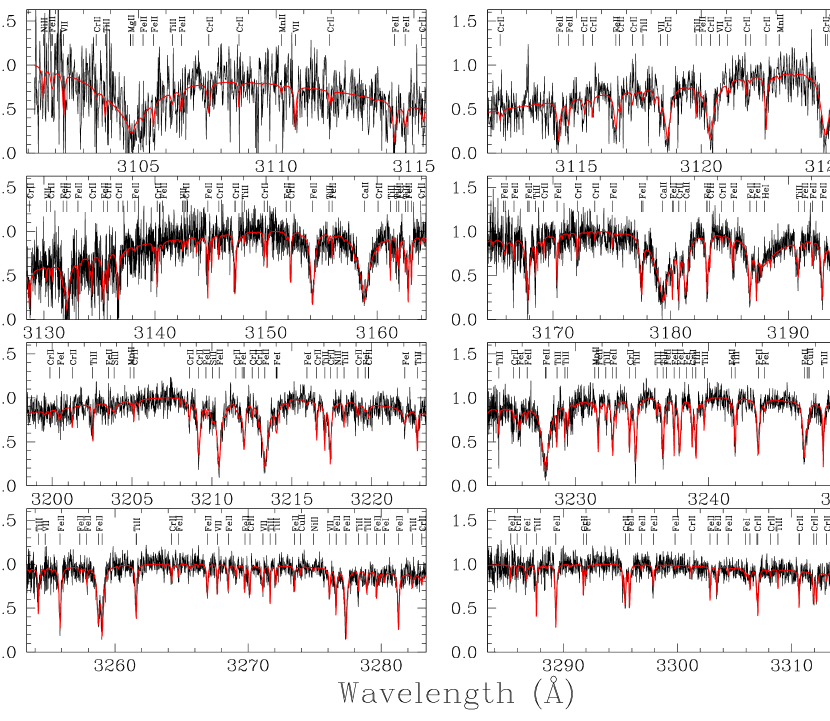
Figure 6.— Display of our final solution (in red) over the most interesting HIRES orders. Ticks and labels identify the strongest features present in the spectra. The observations have been artificially shifted to air wavelengths in order to facilitate line identification using available line lists.

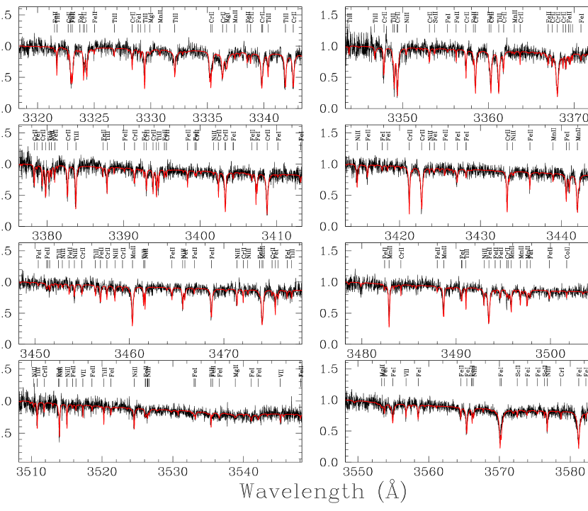
Figure 7.— Same as previous Figure.

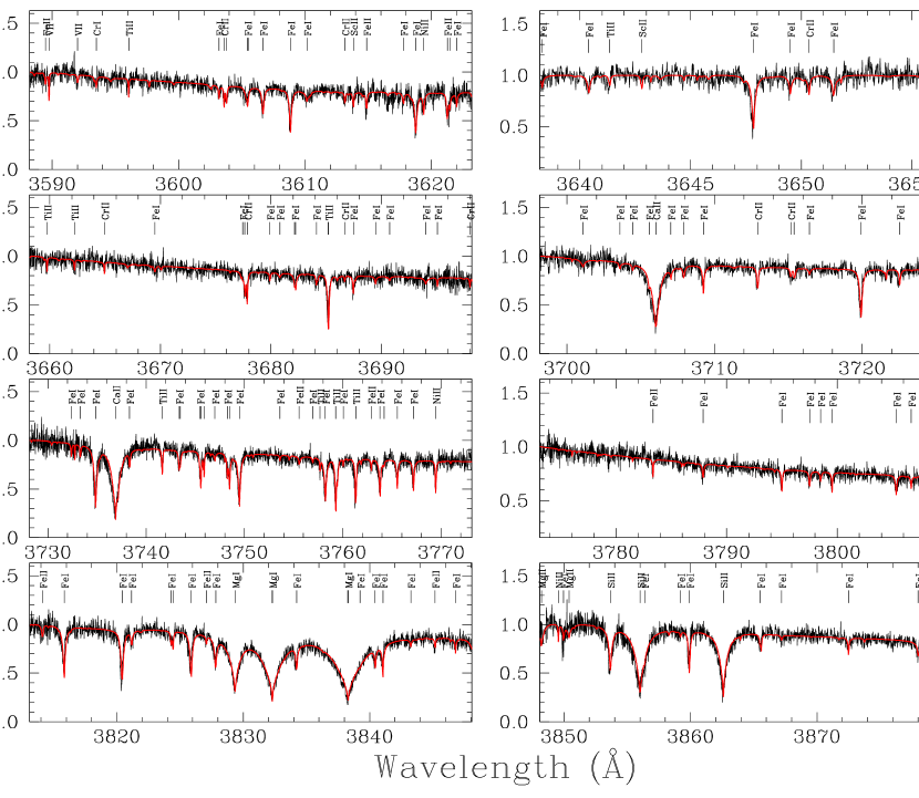
Figure 8.— Same as previous Figure.

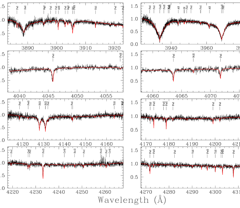
Figure 9.— Same as previous Figure.

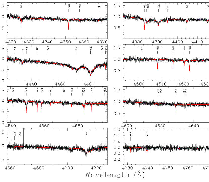
Figure 10.— Same as previous Figure.

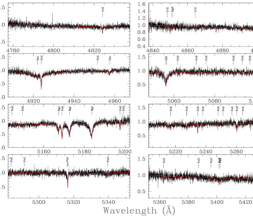
Figure 11.— Same as previous Figure.

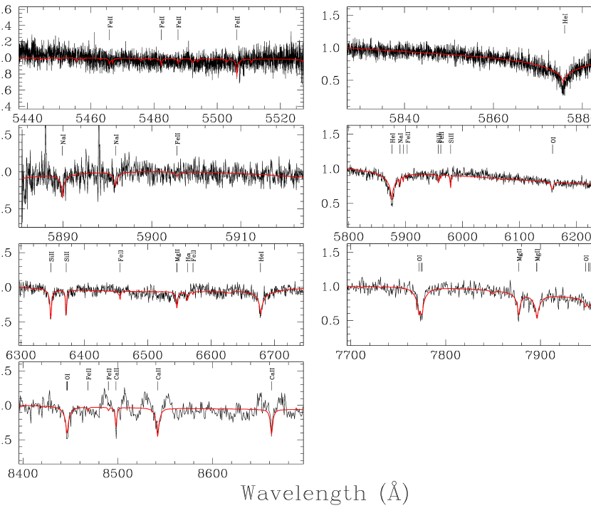
Figure 12.— Same as previous Figure. The last five panels display MagE spectroscopic data. The double-peaked gas disk emission features of CaII first reported by Gänsicke (2011) are evident in the last panel.

We also, a posteriori, verified explicitly that this new solution was still compatible with the lower resolution MMT spectroscopic data used in Dufour et al. (2010). Figure 13 shows that the slight change in atmospheric parameters that we derive here did not have any noticeable impact on the quality of the fit to the various HeI lines in our ”old” MMT data. In fact, we even observe that most of the discrepancies in the predicted line strengths of Fe lines (see Dufour et al., 2010, Figure 3) are now almost completely removed. We attribute this result on our improvement in the atmospheric parameters as well as the use of better atomic line data (VALD).

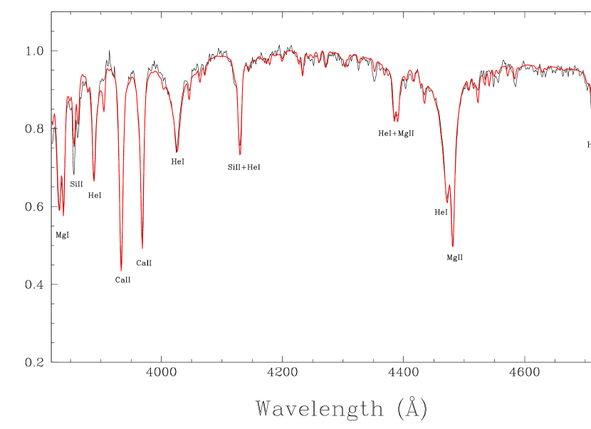
Figure 13.— Display of our final solution (in red) over the lower resolution MMT data used in Dufour et al. (2010, see their Figure 3). The strongest lines are identified while all the other numerous non-identified lines are from iron. The discrepancies in Fe line strengths noted by Dufour et al. (2010) have almost all disappear (see text).

It is interesting to note that while the HeI line profiles seem well reproduced by our models when observed at relatively low resolution, such is not the case at higher resolution. Indeed, detailed inspection of strong HeI line at $\lambda\lambda$ 3889, 4471, 4713, 4922 and 5876 indicates that the synthetic models poorly reproduce the HIRES observations (the MagE observations of HeI $\lambda\lambda$ 5876 and 6678, taken at lower resolution, are more satisfactory). Similar problems in HeI line profiles have also been observed in other cool DBZ white dwarfs (see, in particular, the narrow absorption core component in HeI $\lambda$5876 for GD 362, GD 16 and PG 1225$-$079, Zuckerman et al., 2007; Klein et al., 2011). Note that varying the atmospheric parameters ($T_{\rm eff}$/$\log g$) from the optimal values determined above does not improve our fit to the helium lines; the discrepancy appear to reside in the predicted line shape. The explanation for the features morphology eludes us at this time. Until this issue is resolved, we believe it is safer to use the ionization balance of heavy elements to obtain the effective temperature and surface gravity with high precision

We also present in Figure 14 a similar exercise using unpublished $\approx$1 Å resolution MMT spectroscopic observations that covers the bluer part of the electromagnetic spectrum. While the signal-to-noise ratio and resolution of these observations were first judged to be insufficient to provide significant improvements over Dufour et al. (2010)’s solution, they are nevertheless useful to confirm that no significant change in the elemental abundances of the major species has occurred between the $\sim$1 year that separates the MMT and Keck observing runs. This is not surprising given that this object is most probably accreting material at a steady state and that the diffusion timescales of the heavy elements are of the order of $10^{5}$ years (see below).

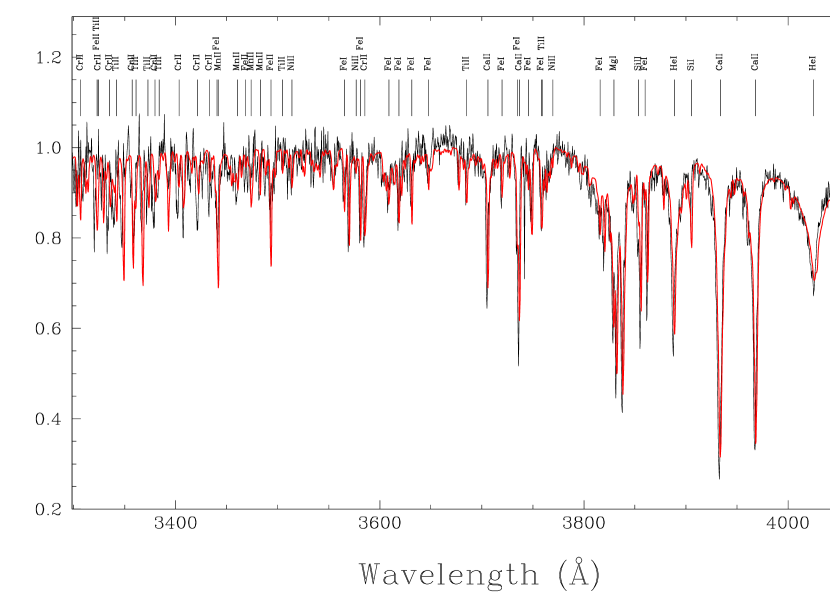
Figure 14.— Display of our final solution (in red) over new unpublished medium resolution MMT data. Ticks and labels identify the strongest features present in the spectra.

Although the final abundance determination has been obtained only from an average of a subsample of all the lines present in the Keck and Magellan spectroscopic datasets, we find that the synthetic spectrum calculated with our final solution agrees remarkably well with the observations for the vast majority of the lines over the whole spectrum (see Figures 6 to 12). This can most probably be attributed to the fact that the method described above has yielded a very accurate set of atmospheric parameters that minimized the dispersion among the set of individual measurements. Indeed, we find that the standard deviation of the set of individual measurements for a given element vary typically between 0.04 to 0.10 dex (with a few exceptions, notably oxygen, that have slightly larger dispersions; see below).

There are, however, a few individual lines which significantly depart from our final optimal solution (most probably due to discrepancies in atomic line data or broadening parameters). These can be observed in Figures 6 to 12 as features that are not very well reproduced by the final synthetic spectrum (see, for example, lines near $\lambda\lambda$4370, 4740, 4850, 5400, 5505). Overall, fortunately, the final atmospheric parameters are not significantly affected by these lines since their contribution tend, for the few included in the final set, to be averaged out from using multiple lines from each elements (O, Na, Al, Sc and Co, which rely on 3 or less individual measurements, must thus be considered more uncertain on that account).

We note, finally, that our observations for J0738+1835 show no sign of emission cores in the CaII H&K lines, as observed for PG 1225$-$079 (Klein et al., 2011). Klein et al. (2011) proposed that NLTE effects could possibly cause such emission since these line cores are formed high up in the atmosphere. However, comparing the thermodynamic structures of PG 1225$-$079, calculated with Klein et al. (2011)’s parameters, with that of J0738+1835 argues against this interpretation (not to mention that NLTE effect are not expected in such a low effective temperature white dwarf). Indeed, we find that the atmospheric pressure in J0738+1835 is lower than that of PG 1225$-$079, while its gas temperature is higher at every depth point in the atmosphere. Since both of these should favor NLTE effects (less collisions and a more intense radiation field), if NLTE was the explanation, J0738+1835 (and other similar DBZ white dwarfs) would be even more likely to show cores in emission. Since they are not observed in any other object, PG 1225$-$079 is more likely a unique and interesting case of white dwarf chromospheric activity.

It is interesting to note, however, that our MagE spectroscopic observations clearly show evidence of the IR CaII double-peaked emissions (see Figure 12). These features, which were already observed in the SDSS spectroscopic data (see Gänsicke, 2011), are the typical signature of gaseous debris disks rotating around a white dwarf (Gänsicke et al., 2006, 2007, 2008).

It has been proposed that gas disk-hosting systems could be the result of multiple infalling bodies originating from a solar system-like asteroid belt (Jura, 2008). However, the total mass of heavy element presently found in J0738+1835’s convective zone represent a very large fraction of the mass of an asteroid belt. While it is possible to explain this large amount by the accretion of several small asteroids, as newly-shredded asteroids dust arrives near the pre-existing disk, destructive grain-grain collisions should rapidely cause the disk to evolve toward a large gaseous system (Jura, 2008). Given that a significant dusty disk component is revealed from a large infrared excess (see below), we are most likely withnessing a case where one large object generated the dense dust disk which dominate the system and that the small amount of gas observed is the result of much smaller bodies hitting the dust disk from time to time. It is also possible that we are watching the system in a transition phase where the dusty disk is starting to slowly dissipate, through internal motions, into a gaseous phase. Alternatively, the emission line flux could be understood, as proposed by Gänsicke (2011), by some heating of the top layers of the disk with ultraviolet photons from the white dwarf (see also Melis et al., 2010). Unfortunately, our understanding of white dwarfs debris/gaseous disk is insufficient at this point to speculate furthermore on the formation/evolution of these components.

3.2. Infrared Excess and Disk Model

The presence of an accretion disk around J0738+1835 was unambiguously established from $JHK$ excess photometry in Dufour et al. (2010). However, due to the lack of mid-infrared data, the outer temperature was not well constrained. Here we use Spitzer (IRAC) 3.6 and 4.5 $\mu$m data combined with Gemini JHK photometry to get better constraints on the physical parameters of the disk.

In the same manner as in Dufour et al. (2010), we use the optically thick flat-disk models of Jura (2003) and determine the best fit disk parameters. We obtain $T_{in}=1600\pm 100$ K, $T_{out}=900^{+100}_{-200}$ K and an inclination angle of 40 $\pm$ 20 degree (see Figure 15). The uncertainties for these parameters were obtained following the method described in Kilic et al. (2011). Briefly, a Monte Carlo analysis is performed where the observed photometric fluxes f are replaced with f + g$\delta$f, where $\delta$f is the error in flux and g is a Gaussian deviate with zero mean and unit variance. For each of 10,000 sets of modified photometry, the analysis is repeated to derive new best-fit parameters for the disk. The interquartile range of these parameters is adopted as the uncertainty. The larger low range uncertainty found for the outer temperature is the result of not having data beyond 5 microns since it is possible that the disk may extend to larger radii with a corresponding cooler lower-limit for the temperature. With $T_{out}=900$ K, corresponding to an outer radii of $\sim$ 0.1 R_⊙, the disk is well placed inside the tidal radius of the white dwarf ($\sim$ 1 R_⊙), further strengthening the idea that the origin of the disk, as well as the material polluting the white dwarf’s convection zone, is the tidal disruption of a large rocky body.

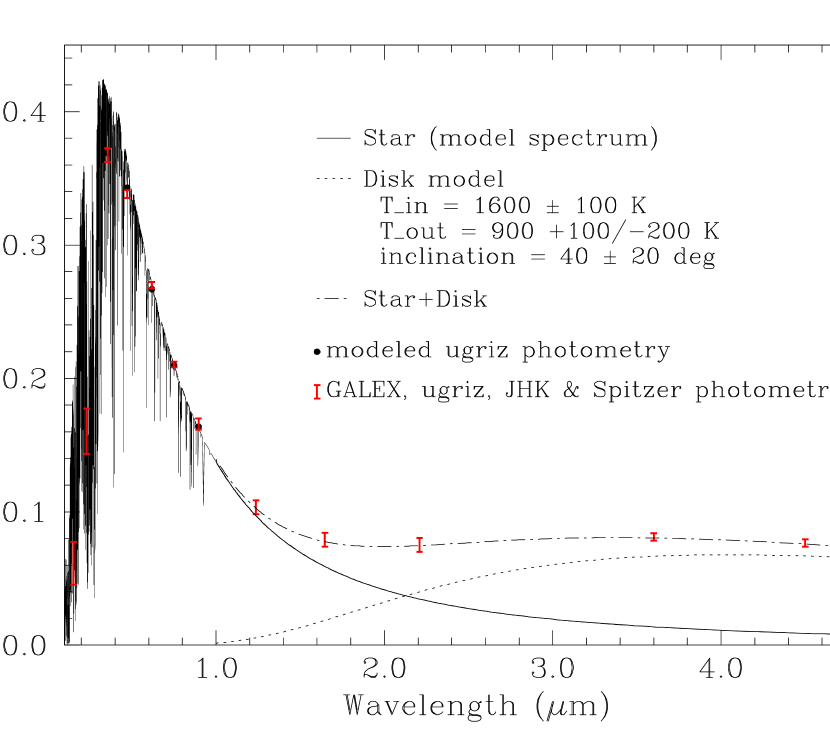
Figure 15.— Photometric measurements in GALEX, ugriz, $JHK$ and Spitzer 3.6 $\mu$m and 4.5 $\mu$m bands compared to the models of the star and the debris disk.

4. RESULTS AND DISCUSSION

As discussed in details in Koester (2009), the interpretation of the abundance pattern measured at a white dwarf photosphere is not always straightforward. Indeed, depending in which of the three phases of the accretion-diffusion process the star is observed (which we generally do not know, especially in the case of helium-rich atmosphere white dwarfs with relatively long diffusion timescales), the relation between the photospheric abundance and that of the accreted body differs.

For instance, in the first phase, when the accretion process just began, the observed relative abundance of each element measured at the photosphere directly translates into that of the polluting body. Next, the so-called steady state is reached and the abundance pattern can no longer be directly interpreted since each element has its own characteristic diffusion timescale. Fortunately, one can still recover the relative abundance of the source material by simply applying a correction that takes into account the difference in diffusion time of the various elements (see Dupuis et al., 1993). Finally, when the accretion ends, each element disappears exponentially with their corresponding diffusion constant, quickly affecting the abundance ratios between elements with different timescales. In the case of J0738+1835, given the strength of the infrared excess, as well as the large accretion rates needed to explain the photospheric pollution (see Table 2), one can be confident that this system is currently accreting and not in the declining phase.

It is generally assumed that systems with important infrared excess are in the steady state regime, although there is always a small chance that we are observing this object in the early phase. The probability of catching an object at that moment depends on the disk lifetime, which is, however, highly uncertain. Based on simple assumptions, Jura (2008) estimates that a median-sized asteroid may produce a disk that last around $1.5\times 10^{5}$ yrs, comparable to the diffusion timescales of the heavy elements in J0738+1835’s photosphere (see below). If dusty disk lifetimes are truly that short, then the steady state might not be reached and the observed abundance pattern could be directly interpreted. However, it is also possible that dusty disks, depending on their viscosity and composition, may last as long as $10^{8}$ yrs, like the rings of Saturn. Accordingly, given our poor understanding of the temporal evolution of circumstellar disks, caution is well advised when interpreting observed abundance ratios (for example, see Rafikov, 2011; Jura12). The presence of a gaseous component, however, seem to indicate that J0738+1835’s disk will probably evolve much faster than that. Nevertheless, assuming that a much larger body such as the one that was tidally disrupted near J0738+1835 could last longer (a few settling time) than the simple estimates of Jura (2008), then a steady state could be reached.

In any case, the maximum correction applicable on the abundance ratio of two elements in the steady state regime is only $\sim$1.6 (see below) for J0738+1835’s atmospheric parameters, and our conclusions are not significantly affected by the exact regime in which J0738+1835 is assumed to be. For simplicity, we will thus simply assume that J0738+183 is accreting material in the steady state regime for the rest of our discussion.

4.1. Convection Zone Models and Diffusion Timescales

The convection zone models for our present analysis of J0738+1835 have been built as described in Dufour et al. (2010). In brief, we computed full stellar structures specified by the values of their surface gravity and effective temperature (to ease comparison with the spectroscopic observations), as well as a chemical stratification given by a He-rich ($Z$ = 0.001) outer layer of fractional mass log ($1-M(r)/M_{*}$) = $-$3.0 surrounding a C/O core. Given the relative insensitivity of the convection zone thickness on the assumed convective efficiency for the atmospheric parameters appropriate for J0738+1835 (see Dufour et al. 2010), we only considered the so-called ML2/$\alpha$=1.0 version in the present paper. Convection zone models were thus computed for five values of the effective temperature ($T_{\rm eff}$= 13,000 K to 14,200 K, in steps of 300 K), and five values of the surface gravity ($\log g$= 8.1 to 8.9, in steps of 0.2 dex). This domain in parameter space is centered on the atmospheric parameters for J0738+1835 initially inferred in Dufour et al. (2010), and more than cover the uncertainty range ultimately found in the present study.

The spline coefficients provided by Paquette et al. (1986a) to characterize the collision integrals involved in diffusion processes have been widely used in stellar astrophysics. In the case of white dwarfs, they have first been used by Paquette et al. (1986b) to estimate the diffusion timescales of a few representative metals at the base of the convection zone of sufficiently cool He- and H-rich stars. The exact same approach has been followed recently by Koester (2009) for additional elements, including the use of the same rough model of pressure ionization devised by Paquette et al. (1986b) for estimating the average charge of trace heavy elements under white dwarf conditions. Given the importance of investigating the presence of trace amounts of metals in cool white dwarfs in the context of the new paradigm of a planetary origin, our group at Montréal has gone back to the basic problem of computing still more realistic diffusion coefficients. The details of this effort will be reported elsewhere, but we point out here that 1) improvements in the numerical evaluations of the collision integrals have been implemented, 2) a more physical description of the screening length has been used, 3) an improved model of pressure ionization (insuring smoothness of the charge of an element with depth) has been adopted, and 4) all 27 elements from Li to Cu in the periodic table have been considered in the calculations.

Figure 16 summarizes our computations of settling timescales at the base of the convection zone for our He-rich white dwarf models. In the range of effective temperatures depicted, the diffusion timescale for a given element increases monotonically with decreasing temperature at fixed gravity, but the effect is relatively small. On the other hand, in the range of surface gravity considered in Figure 16, the diffusion timescale increases relatively quickly with decreasing surface gravity at fixed temperature. We note that, while the diffusion timescales can vary significantly with changing atmospheric parameters, the ratios of timescales between any two elements are much less sensitive.

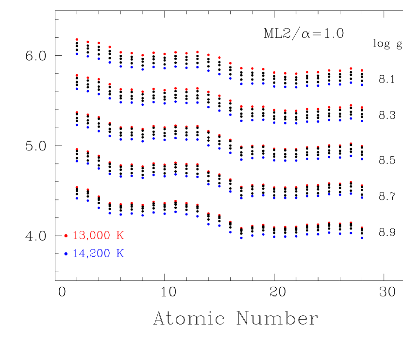
Figure 16.— Diffusion timescale for all elements from Li to Cu (atomic number 3 to 29). Steps of 300 K in effective temperature and 0.2 dex in $\log g$.

4.2. Bulk Composition and Hydrogen

The derived quantities (abundances, total amount of material found in the helium convection zone, settling timescales, steady state ratios and accretion rates) presented in Table 2 reveal a number of interesting properties about the body that polluted J0738+1835’s photosphere. Not surprisingly, the total amount of heavy elements is found to be mainly concentrated in the four major constituent of large rocky bodies like Earth (O, Mg, Si and Fe) with proportions similar to those found for the most polluted and well studied helium-rich white dwarfs GD 362, GD 40 and HS2253+8023 (Zuckerman et al., 2007; Klein et al., 2010, 2011). In total, there is some $6.6\times 10^{23}$ g of accreted material currently present in the helium convection zone, the largest amount directly detected at the photosphere of a white dwarf. The object that tidally disrupted near J0738+1835 was thus at least as massive, and probably even more massive, than the dwarf planet Ceres. Assuming a typical density of $\sim$ 2.1 g/cm³, the alleged planet radius was at least 400 km, and most probably much more considering the unknown amount of material that i) has already sunk below the convection zone and ii) is still contained in the surrounding debris disk.

Inspection of Table 2 also reveals a very low amount of hydrogen, implying that this dwarf planet was very dry, with less than 1% of the total mass coming from water ice (note that this is an upper limit since hydrogen, the lightest element, can only accumulate at the surface of the white dwarf with cooling age). According to Jura & Xu (2010), most of the internal water ice present in a 400 km object should survive the late stage of evolution. The low amount of hydrogen found at J0738+1835’s photosphere can thus safely be interpreted as a reflection of the low amount of water ice initially contained in the accreted object. Hence, the body responsible for J0738+1835’s metal pollution must have formed inside the so-called ”snow line” where the thermodynamic conditions are such that rocky planetesimals initially possess little to no water (a similar conclusion was also recently found for a large sample of nearby helium-rich white dwarfs, see Jura & Xu, 2012).

4.3. Oxygen Budget and Temperature Trends

Oxygen accounts for more than half of the material accreted onto the surface of J0738+1835. Another way to strengthen the rocky nature of the polluting body is to verify that all the accreted oxygen can by accounted for assuming it is contained in rocky oxygenated minerals (Klein et al., 2010). In other words, if the oxygen was all contained in mineral oxides (such as MgO, $\rm Al_{2}O_{3}$, $\rm SiO_{2}$, CaO, $\rm TiO_{2}$, $\rm Cr_{2}O_{3}$, MnO, FeO, $\rm Fe_{2}O_{3}$, and NiO) would the abundance of all the heavy elements found in the photosphere add up in sufficient quantity to explain the oxygen abundance? Quantitatively, this corresponds to (see equation 3 of Klein et al., 2010):

$$\frac{1}{2}\frac{n(H)}{n(O)}+\sum_{Z}\frac{q(Z)}{p(Z)}\frac{n(Z)}{n(O)}=1.$$ (1)

where the heavy element Z is contained in molecule $Z_{q(Z)}O_{p(Z)}$. Using the values presented in Table 2, we calculate the steady state ratios and find that the sum adds up only to around $\sim$ 0.4 depending on how we divide Fe into $\rm Fe_{2}O_{3}$ and FeO. Taken at face value, this indicates an oxygen overabundance, something that is difficult to explain given the severe constraint we have, from the low amount of hydrogen, on the water content of the accreted body.

However, as noted above, the oxygen abundance is based only on 3 individual measurements which are quite discrepant between one another (it is not clear at this point whether this is due to the relatively lower resolution and signal-to-noise ratio of the observations or discrepancies in atomic line data/broadening parameters). Since one of these measurements gives an abundance of log O/He = -4.1 (the other two give -3.85 and -3.61), which is low enough to reconcile the oxygen budget, we could be tempted, until more precise measurements become available, to prefer the low end value in the abundance range permitted by the uncertainty.

Alternatively, the unusually high oxygen abundance could be explained by the local thermodynamical condition of the protoplanetery disk at the distance where the object formed. For instance, since the equilibrium composition of planetesimal embryos vary with temperature and pressure at different radii (Bond et al., 2010a, b), one expect, in a cooler environment, to observe a decrease in the abundances of the most refractory elements such as Al and C, as well as an increase in more volatile elements like O . It is thus possible that most of the oxygen was actually locked up in more complex molecules than those assumed above ($\rm MgAl_{2}O_{3}$, $\rm NaAlSi_{3}O_{8}$ for example), which would help to bring the oxygen balance nearer to 1.

Interestingly, if the accreted object formed from fractionated disk material whith different thermodynamical conditions than where Earth formed, then it might also be possible to observe a signature of this in the form of a correlation in the abundance ratios with condensation temperatures. Such correlations have been searched for in some heavily polluted and well studied helium-rich white dwarfs such as GD 40, PG 1225$-$079 and HS 2253+8023 (Klein et al., 2010, 2011).

In the case of GD 40 and PG 1225$-$079, the refractory elements are substantially enhanced relative to Mg and Earth values. The detailed simulations of Bond et al. (2010a) indicate that planets forming in hotter regions than where Earth formed will be rich in refractories but low in other elements such as Mg, Si, O and Fe. For the objects analyzed by Klein et al. (2010, 2011), this is observed for Si, but not for Mg and Fe, suggesting that other processes could also be important. For instance, there could have been intense heating in the red giant phase, silicate vaporization, or even crust removal that could have affected the final bulk abundances in the bodies that accreted onto these stars. Consequently, although the planetary compositions derived in these stars suggest close formation to the host star, explaining the observed abundance pattern as a whole still remains quite challenging.

With 14 heavy elements detected and measured in its photosphere, J0738+1835 provides us with a unique opportunity to empirically observe in greater details the abundance pattern for another large terrestrial-like planet. Following Klein et al. (2011, see their Figure 18), we plot in Figure 17 the observed abundances, normalized to Mg and bulk Earth, as a function of the condensation temperatures of each element (taking Fe, instead of Mg, as a reference produces a very similar plot while using Si shifts the points upward by about a factor of 1.5). Our measurements suggest that there is indeed a correlation of the abundance ratios with condensation temperature, highly refractory elements being depleted (relative to bulk Earth) while the most volatile elements appear enhanced. We note that the presence of this trend with condensation temperature depends little on whether we assume that the accretion occurs in the early phase or at steady state (in which case a small correction, consisting of simply multiplying the results by the ratios of the diffusion times of the considered elements, is applied). The pattern for the most refractory elements is completely the opposite to what was found for GD 40 and PG 1225$-$079, clearly indicating a different formation history and/or subsequent evolution of the body responsible for J0738+1835’s metal pollution.

Figure 17.— Abundances relative to magnesium and bulk Earth (Allègre et al., 2001) as a function of 50% condensation temperature (Lodders, 2003). The error bars are plotted only for the steady state ratios for clarity (early phase error bars are essentially the same). The dotted line is a best least square fit to the steady state ratios while the dashed line is to guide the eye to Earth-like values.

Recent simulations of the formation of terrestrial planets by Bond et al. (2010a) suggest that objects forming in the inner regions have high Mg/Si, Al/Si and Ca/Si ratios with a steady transition toward Earth’s values as one moves further out. This trend is a reflection of the condensation of refractory species in the inner most region and of Mg-silicate further out. The low abundances that we find for many refractory species could thus indicate that the planet/asteroid that polluted J0738+1835 formed further out in cooler regions where the Ca- and Al-rich inclusions (CAI), as well as other refractory-rich material, cannot condensate out easily.

Although this simple interpretation is appealing to explain our results, a few problems remain. For instance, according to Bond et al. (2010a)’s simulations, while Al is condensing out in the inner regions of the disk, Na and Al are expected to condense further out together (species such as $\rm MgAl_{2}O_{3}$ and $\rm NaAlSi_{3}O_{8}$ condense out over a similar temperature range as Mg silicates). Hence, it is not clear how it could be possible to deplete Al and Si but not Na (a similar argument can be applied to Mn as well).

It must be noted, however, that the error bars on some of these elements are quite large, severely affecting our level of confidence on the existence of the trend for the low range of condensation temperature ($\rm T_{c}<1200$ K). In particular, Na and Mn abundances rely on very few measurements and given the signal-to-noise ratio of our observations in the region where these lines are found (and the corresponding error bars), it is quite possible that the real abundances of these elements could lie on the low end range of our measurements, which would be more compatible with Earth-like values. Furthermore, it must be noted that the estimation of the composition of bulk Earth volatile material is quite a difficult task (see Allègre et al., 1995, 2001) and that uncertainties on the Na and Mn Earth values used for the normalization in Figure 17 are to be considered as well. For example, taking Na and Mn values from Allègre et al. (1995) over those of Allègre et al. (2001) would lead to a better agreement between the observed abundances of these elements and Earth values.

Since, as we discussed above, the oxygen abundance is also quite uncertain (the lower abundance of oxygen would also be more compatible with the oxygen balance argument in certain conditions), another coherent picture could be that the observed abundances are in fact close to Earth values for most elements, with only a few exceptions like Si, Ti and Al, which can confidently be considered depleted relative to bulk Earth.

Such a pattern, if confirmed with better accuracy, could be interpreted very differently. For example, it is possible that differentiation took place in the body that accreted at the surface of J0738+1835 (in fact, with a minimal radius of at least 400 km, differentiation most probably occurred). As discussed in Klein et al. (2010), elements such as Si, Ca, Ti, Al tend to concentrate in the crust of a differentiated body. Given that it is these very same elements that are found to be depleted in our object, the abundance pattern found in J0738+1835’s photosphere could very well be due to some sort of crust removal. A similar process may explain the strange abundance pattern found in GALEX J1931+0117 (Melis et al., 2011), where the planet’s outer layers is believed to have been stripped away by some wind interaction in the AGB phase. Another possibility would be that a large impact striped away a large portion of the crust, affecting the final composition that we observe at the white dwarf photosphere (see Zuckerman et al., 2011, where a similar scenario has been proposed to explained the peculiar abundances found in NLTT 43806).

It is unfortunate that a detailed analysis such as this one, even using data from some of the best observational facilities in the world, cannot discriminate furthermore between the different possible scenarios. Although our analysis clearly indicates that the most refractory elements are depleted relative to Mg and Earth, the case for a trend with condensation temperature must be considered more speculative at this point due to the uncertainties in our measurements. .

Future investigation aiming at refining, among other things, the oxygen, sodium and manganese abundances, should help to rule out some of the various scenarios described above. Meanwhile, until better spectroscopic observations become available, we prefer to remain cautious and not overinterpret the data. Regardless, our study seems to indicate that that we are on the verge of entering an exciting new era of high precision measurements of terrestrial-like planet compositions from polluted white dwarfs and that appreciable insights on planetary formation should be accessible in the near future..

5. CONCLUSION

We presented a detailed analysis, based on high resolution optical spectroscopic observations, of the DBZ SDSS J073842.56+183509.06, the most metal polluted white dwarf currently known. We also obtained IRAC Spitzer infrared photometry at 3.6 $\mu$m and 4.5 $\mu$m, which, combined with earlier $JHK$ photometric measurements, allows us to better constrain the properties (inner and outer temperature, inclination) of the bright debris disk surrounding that white dwarf.

We have measured the abundances of 14 different heavy elements and determined that the total mass of material currently present in the helium convection zone is $\sim 6.6\times 10^{23}$ g, indicating that the object that was tidally disrupted was at least as large as the dwarf planet Ceres. We also find, from the low amount of hydrogen present in the photosphere, that the total amount of water ice was less the 1% of the mass of this object, suggesting that it formed inside the so-called snow line.

Our most interesting finding, summarized in Figure 17, is that the highly refractory species are depleted, relative to Mg and Earth, while more volatile elements appear to be enhanced, with a possible correlation with the condensation temperature. Such a trend could be the signature that the dwarf planet that accreted on J0738+1835 formed in a lower temperature environment than Earth, where the thermodynamical conditions are such that the planetesimal embryos’ chemical composition tends to be depleted of more refractory elements. However, the correlation must be considered uncertain given the large uncertainties associated with the O, Na and Mn measurements. Nevertheless, it is clear that the Si/Mg, Ti/Mg and Al/Mg ratios are lower than bulk Earth values, indicating that the physical processes that affected the final composition of the dwarf planet were different than those that occurred for Earth and other polluted white dwarfs such as GD 40, GD 362 and PG 1225$-$079.

Another way to interpret our findings, if we momentarily ignore the more uncertain O, Na and Mn abundances, is that differentiation occurred in the large body that produced the pollution observed on J0738+1835. With a radius of at least 400 km, a crust containing preferentially Si, Ti, Al and Ca could have formed and been removed, potentially explaining part of the abundance pattern that we find.

Improvements, allowing us to discriminate between these various scenarios, albeit difficult, should be obtainable from longer observing runs on large telescopes (the combination of high resolution with high signal-to-noise ratio is the key to obtain precise results). This work, as well a many other recent studies (for example, Zuckerman et al., 2007, 2010; Melis et al., 2011; Klein et al., 2010, 2011) demonstrate, once more, the extraordinary potential of metal contaminated white dwarfs to study rocky extrasolar planet/asteroid bulk compositions. These objects are unique probes that can serve as perfect testbeds for planetary formation and evolution theories, providing information that cannot be obtained from any other way. As our understanding of the physical processes at play increases, as well as our confidence in the interpretation of the chemical patterns found in these stars, reliable bulk composition of rocky extrasolar objects, conceivably with a level of precision comparable, if not better, to what is possible for similar objects in the solar system, should soon be provided from metal polluted white dwarf studies.

References

- Allègre et al. (1995) Allègre, C. J., Poirier, J.-P., Humler, E., & Hofmann, A. W. 1995, Earth and Planetary Science Letters, 134, 515
- Allègre et al. (2001) Allègre, C., Manhès, G., & Lewin, E. 2001, Earth and Planetary Science Letters, 185, 49
- Bochanski et al. (2009) Bochanski, J. J., Hennawi, J. F., Simcoe, R. A., et al. 2009, PASP, 121, 1409
- Bond et al. (2010a) Bond, J. C., O’Brien, D. P., & Lauretta, D. S. 2010, ApJ, 715, 1050
- Bond et al. (2010b) Bond, J. C., Lauretta, D. S., & O’Brien, D. P. 2010, icarus, 208, 504
- Debes & Sigurdsson (2002) Debes, J. H., & Sigurdsson, S. 2002, ApJ, 572, 556
- Dufour et al. (2007) Dufour, P., et al. 2007, ApJ, 663, 1291
- Dufour et al. (2010) Dufour, P., Kilic, M., Fontaine, G., Bergeron, P., Lachapelle, F.-R., Kleinman, S. J., & Leggett, S. K. 2010, ApJ, 719, 803
- Dupuis et al. (1993) Dupuis, J., Fontaine, G., Pelletier, C., & Wesemael, F. 1993, ApJS, 84, 73
- Farihi (2011) Farihi, J. 2011, American Institute of Physics Conference Series, 1331, 193
- Farihi et al. (2010a) Farihi, J., Barstow, M. A., Redfield, S., Dufour, P., & Hambly, N. C. 2010, MNRAS, 404, 2123
- Farihi et al. (2010b) Farihi, J., Jura, M., Lee, J.-E., & Zuckerman, B. 2010, ApJ, 714, 1386
- Farihi et al. (2009) Farihi, J., Jura, M., & Zuckerman, B. 2009, ApJ, 694, 805
- Fazio et al. (2004) Fazio, G. G., Hora, J. L., Allen, L. E., et al. 2004, ApJS, 154, 10
- Fontaine et al. (2001) Fontaine, G., Brassard, P., & Bergeron, P. 2001, PASP, 113, 409
- Gänsicke (2011) Gänsicke, B. T. 2011, American Institute of Physics Conference Series, 1331, 211
- Gänsicke et al. (2008) Gänsicke, B. T., Koester, D., Marsh, T. R., Rebassa-Mansergas, A., & Southworth, J. 2008, MNRAS, 391, L103
- Gänsicke et al. (2007) Gänsicke, B. T., Marsh, T. R., & Southworth, J. 2007, MNRAS, 380, L35
- Gänsicke et al. (2006) Gänsicke, B. T., Marsh, T. R., Southworth, J., & Rebassa-Mansergas, A. 2006, Science, 314, 1908
- Gianninas et al. (2004) Gianninas, A., Dufour, P., & Bergeron, P. 2004, ApJ, 617, L57
- Hamuy et al. (1994) Hamuy, M., Suntzeff, N. B., Heathcote, S. R., et al. 1994, PASP, 106, 566
- Jura (2003) Jura, M. 2003, ApJ, 584, L91
- Jura (2006) Jura, M. 2006, ApJ, 653, 613
- Jura et al. (2007) Jura, M., Farihi, J., & Zuckerman, B. 2007, ApJ, 663, 1285
- Jura (2008) Jura, M. 2008, AJ, 135, 1785
- Jura & Xu (2010) Jura, M., & Xu, S. 2010, AJ, 140, 1129
- Jura & Xu (2012) Jura, M., & Xu, S. 2012, AJ, 143, 6
- Kilic et al. (2011) Kilic, M., Patterson, A. J., Barber, S., Leggett, S. K., & Dufour, P. 2011, arXiv:1110.3799
- Klein et al. (2010) Klein, B., Jura, M., Koester, D., Zuckerman, B., & Melis, C. 2010, ApJ, 709, 950
- Klein et al. (2011) Klein, B., Jura, M., Koester, D., & Zuckerman, B. 2011, ApJ, 741, 64
- Koester (2009) Koester, D. 2009, A&A, 498, 517
- Kupka et al. (1999) Kupka, F., Piskunov, N., Ryabchikova, T. A., Stempels, H. C., & Weiss, W. W. 1999, A&AS, 138, 119
- Kupka et al. (2000) Kupka, F. G., Ryabchikova, T. A., Piskunov, N. E., Stempels, H. C., & Weiss, W. W. 2000, Baltic Astronomy, 9, 590
- Lodders (2003) Lodders, K. 2003, ApJ, 591, 1220
- Marshall et al. (2008) Marshall, J. L., Burles, S., Thompson, I. B., et al. 2008, Proc. SPIE, 7014,
- Massey et al. (1988) Massey, P., Strobel, K., Barnes, J. V., & Anderson, E. 1988, ApJ, 328, 315
- Melis et al. (2011) Melis, C., Farihi, J., Dufour, P., et al. 2011, ApJ, 732, 90
- Melis et al. (2010) Melis, C., Jura, M., Albert, L., Klein, B., & Zuckerman, B. 2010, ApJ, 722, 1078
- Paquette et al. (1986a) Paquette, C., Pelletier, C., Fontaine, G., & Michaud, G. 1986a, ApJS, 61, 177
- Paquette et al. (1986b) Paquette, C., Pelletier, C., Fontaine, G., & Michaud, G. 1986b, ApJS, 61, 197
- Piskunov et al. (1995) Piskunov, N. E., Kupka, F., Ryabchikova, T. A., Weiss, W. W., & Jeffery, C. S. 1995, A&AS, 112, 525
- Rafikov (2011) Rafikov, R. R. 2011, MNRAS, 416, L55
- Reach et al. (2009) Reach, W. T., Lisse, C., von Hippel, T., & Mullally, F. 2009, ApJ, 693, 697
- Reach et al. (2005) Reach, W. T., Kuchner, M. J., von Hippel, T., Burrows, A., Mullally, F., Kilic, M., & Winget, D. E. 2005, ApJ, 635, L161
- Ryabchikova et al. (1997) Ryabchikova, T. A., Piskunov, N. E., Kupka, F., & Weiss, W. W. 1997, Baltic Astronomy, 6, 244
- Vogt et al. (1994) Vogt, S. S., Allen, S. L., Bigelow, B. C., et al. 1994, Proc. SPIE, 2198, 362
- Williams et al. (2009) Williams, K. A., Bolte, M., & Koester, D. 2009, ApJ, 693, 355
- Zuckerman et al. (2003) Zuckerman, B., Koester, D., Reid, I. N., Hünsch, M. 2003, ApJ, 596, 477
- Zuckerman et al. (2007) Zuckerman, B., Koester, D., Melis, C., Hansen, B. M., & Jura, M. 2007, ApJ, 671, 872
- Zuckerman et al. (2010) Zuckerman, B., Melis, C., Klein, B., Koester, D., & Jura, M. 2010, ApJ, 722, 725
- Zuckerman et al. (2011) Zuckerman, B., Koester, D., Dufour, P., et al. 2011, ApJ, 739, 101