Ionization potentials and electron affinities from reduced density matrix functional theory

Abstract

In the recent work of S. Sharma et al., (arxiv.org: cond-matt/0912.1118), a single-electron spectrum associated with the natural orbitals was defined as the derivative of the total energy with respect to the occupation numbers at half filling for the orbital of interest. This idea reproduces the bands of various periodic systems using the appropriate functional quite accurately. In the present work we apply this approximation to the calculation of the ionization potentials and electron affinities of molecular systems using various functionals within the reduced density-matrix functional theory. We demonstrate that this approximation is very successful in general and in particular for certain functionals it performs better than the direct determination of the ionization potentials and electron affinities through the calculation of positive and negative ions respectively. The reason for this is identified to be the inaccuracy that arises from different handling of the open- and closed-shell systems.

I Introduction

It is generally accepted today that the Fermi surfaces of metallic systems obtained with density functional theory (DFT), even at the level of local density approximation (LDA), are in good agreement with experiments. Unfortunately, this is not the case with the band gaps of insulators and semiconductors which are highly underestimated by most of the exchange-correlation (xc) functionals within DFT. Even with the exact xc functional of DFT, the Kohn-Sham (KS) gap is not expected to reproduce the experimental gapGodby et al. (1986). This deviation from experiment is most dramatic for Mott-insulators, most of which are predicted by their KS spectrum to be metallic while they are experimentally known to be insulating in nature.

In this regard reduced density matrix functional theory (RDMFT) has shown great promise in improving on DFT results for a wide class of systems in that it not only improves the KS-band gaps for insulators in general, but also predicts the correct insulating nature for Mott insulators Sharma et al. (2008). Within RDMFT the total energy of a system of interacting electrons is expressed in terms of the one-body reduced density matrix (1-RDM), $\gamma({\bf r},{\bf r}^{\prime})$. This energy functional is then minimized with respect to $\gamma$ under the $N$-representability conditions Coleman (1963) which restrict the minimization to the domain of 1-RDMs that correspond to ensembles of $N$-electron wave functions. A major advantage of RDMFT comes from the fact that the exact kinetic energy is easily expressed as a functional of the 1-RDM of the ground state. In addition, due to the departure from the idempotent single-determinant solution, static electronic correlations are well describedBuijse and Baerends (2002). The total ground-state energy as a functional of $\gamma$ reads (atomic units are used throughout):

$$E[\gamma]= -\frac{1}{2}\int\lim_{{\bf r}\rightarrow{\bf r}^{\prime}}\nabla_{\bf r}^{2}\gamma({\bf r},{\bf r}^{\prime})\,d^{3}{\bf r}^{\prime}+\int\rho({\bf r})\,V_{\rm ext}({\bf r})\,d^{3}{\bf r}$$

$$+\frac{1}{2}\int\frac{\rho({\bf r})\,\rho({\bf r}^{\prime})}{|{\bf r}-{\bf r}^{\prime}|}\,d^{3}{\bf r}\,d^{3}{\bf r}^{\prime}+E_{\rm xc}[\gamma],$$ (1)

where $\rho({\bf r})=\gamma({\bf r},{\bf r})$. $V_{\rm ext}$ is a given external potential, and $E_{\rm xc}$ we call the xc energy functional. In practice, the xc functional is an unknown functional of the 1-RDM and needs to be approximated. A milestone in the development of approximate functionals of the 1-RDM is the Müller functionalMüller (1984); Buijse and Baerends (2002), which has the following form:

$$E_{\rm xc}[\gamma]=E_{\rm xc}[\{\phi_{j}\},\{n_{j}\}]=\\ -\frac{1}{2}\int\int\frac{|\gamma^{1/2}({\bf r},{\bf r}^{\prime})|^{2}}{|{\bf r}-{\bf r}^{\prime}|}\,d^{3}{\bf r}\,d^{3}{\bf r}^{\prime}$$ (2)

where $1/2$ is an exponent in the operator sense. Diagonalization of $\gamma$ produces a set of natural orbitals (the eigenvectors of $\gamma$), $\phi_{j}$, and occupation numbers (the eigenvalues of $\gamma$), $n_{j}$. The Müller functional is known to over correlateStaroverov and Scuseria (2002); Herbert and Harriman (2003); Gritsenko et al. (2005); Frank et al. (2007); Lathiotakis et al. (2007), however, there exist several other approximations most of which are modifications of this functional and are known to improve results for finite systems Goedecker and Umrigar (1998); Lathiotakis et al. (2005); Piris (2006); Leiva and Piris (2005, 2007); Gritsenko et al. (2005); Helbig et al. (2007); Lathiotakis et al. (2007); Pernal (2005); Lathiotakis and Marques (2008); Marques and Lathiotakis (2008); Requist and Pankratov (2008); Piris et al. (2009); Rohr et al. (2008); Lathiotakis et al. (2009a); Piris et al. (2010); Eich et al. (2010); Lathiotakis et al. (2010a); Tolo and Harju (2010); Rohr et al. (2010); Piris et al. (2011).

Several of these RDMFT functionals reproduce the discontinuity of the chemical potential at integer number of electrons which is a measure of the fundamental gap of the systemHelbig et al. (2007); Sharma et al. (2008); Helbig et al. (2009); Lathiotakis et al. (2010b). More precisely, it was demonstrated Helbig et al. (2007, 2009); Lathiotakis et al. (2010b) that the complete removal of the self-interaction (SI) terms leads to discontinuities in the chemical potential that are in good agreement with the fundamental gap for finite systems. Unfortunately, this removal has no effect in the total energy for infinitely extended natural orbitals in periodic systems since their contribution vanishes in the limit of the size of system going to infinity. To overcome this problem, Sharma et al. Sharma et al. (2008) introduced the power functionalSharma et al. (2008); Lathiotakis et al. (2009b) that reproduces discontinuities without requiring the removal of SI terms. This functional has the form

$$E_{\rm xc}[\gamma]=E_{\rm xc}[\{\phi_{j}\},\{n_{j}\}]=\\ -\frac{1}{2}\int\,\int\frac{|\gamma^{\alpha}({\bf r},{\bf r}^{\prime})|^{2}}{|{\bf r}-{\bf r}^{\prime}|}\,d^{3}{\bf r}\,d^{3}{\bf r}^{\prime}$$ (3)

where $\alpha$ is an exponent in the operator sense. The power functional was applied in the calculation of the fundamental gap of various systemsSharma et al. (2008); Tolo and Harju (2010) including transition metal oxides Sharma et al. (2008). An optimal value of $\alpha$ between $0.6$ and $0.7$ was found to reproduce gaps of all systems in close agreement with experiments. These gaps were obtained from the discontinuity of the chemical potential, $\mu(N)$, at an integer total number of electrons $N$. A problem of this method of predicting the gap is that the shape of $\mu(N)$ differs substantially from a step function leading to large error-bars in the prediction of the gap. A second problem is that one needs to calculate the total energy (and $\mu$) for several values of $N$ making the calculation time consuming. Finally, a third problem is that this method does not allow for the calculation of quantities other than the gap, for direct comparison with experiments, like for example the density of states for extended systems and ionization potentials (IPs) and electron affinities (EAs) for finite systems.

An advantage of DFT is that the KS eigenvalues can be used as an approximate single-electron spectrum of the system. Thus, quantities like the IP and EA can be easily estimated using the KS spectrum. A fundamental difference between RDMFT and DFT is the lack of a KS system within RDMFT and the lack of eigenvalue equation makes it difficult to obtain (even approximately) the IPs and the EAs. One way to calculate IPs in RDMFT, is to use extended Koopman’s theorem (EKT), as was proposed by Pernal and CioslowskiPernal and Cioslowski (2005). They demonstrated that the Lagrangian matrix in RDMFT is identical with the generalized Fock matrix entering EKT. Thus, IPs can be calculated by diagonalization of this matrix. They used this idea in the calculation of IPs for small molecular systems using the so called Buijse Baerends Corrected (BBC) Gritsenko et al. (2005) and Goedecker Umrigar (GU)Goedecker and Umrigar (1998) functionals and showed that the error in the obtained IPs is of the order of 4-6%. The same idea was employed in combination with yet another xc functional, namely the PNOF1Piris (2006); Leiva and Piris (2005) functional, for the calculation of the first IPs (FIPs) as well as higher IPs (HIPs) of molecular systems yielding results of similar qualityLeiva and Piris (2006). However, the application of this method is restricted to finite systems, since, for solids, it would require the diagonalization of a large matrix in wave-vector space.

Sharma et al. in Ref. [Sharma et al., 2009] introduced an alternative technique to obtain spectral information. We refer to this technique as the “derivative” (DER) method as it entails for each natural orbital, $k$, the associated energy, $\epsilon_{k}$, be obtained as the derivative of the total energy with respect to the occupation number, $n_{k}$, at $n_{k}=1/2$ and with the rest of the occupation numbers set equal to their ground-state optimal values. This technique has been applied for the calculation of densities of states of transition-metal oxides (NiO, FeO, CoO and MnO) and the results were found to be in excellent agreement with experiments Sharma et al. (2009) and other state-of-the-art many-body techniques like dynamical mean-field theory and the $GW$ method.

In the present work this technique is applied to finite systems. We discuss the validity of the approximations necessary for the accuracy of the method. We present results for the FIP as well as HIP, for atoms and molecules as well as the EAs of atoms, molecules, and radicals adopting several present-day functionals of the 1-RDM. We compare the results with EKT, QCI(T), and experiment.

II theory

Funct.	${\bf\Delta_{\rm DEF}}$(%)	${\bf\Delta_{\rm DIF}}$(%)	${\bf\Delta_{\rm DER}}$(%)
MüllerMüller (1984)	13.24	12.82	10.03
GUGoedecker and Umrigar (1998)	5.90	10.19	9.19
PowerSharma et al. (2008)	12.51	8.68	6.08
AC3Rohr et al. (2008)	5.98	9.33	6.33
PNOF1Piris (2006); Leiva and Piris (2005)	6.27	11.05	7.21
BBC3Gritsenko et al. (2005)	6.24	10.19	8.79
MLMarques and Lathiotakis (2008)	6.15	9.22	4.17

Table 1: Average absolute errors $\Delta_{\rm DEF}$, $\Delta_{\rm DIF}$, and $\Delta_{\rm DER}$, in the calculation of IP, FIPs and HIPs, for a set of atoms and molecules with calculations performed using various xc functionals in conjunction with DEF, DIF, DER methods respectively.

By definition, the ionization potential and electron affinity are given by

$$\begin{array}[]{lcl}{\rm IP}&=&E(N-1)-E(N)\\ {\rm EA}&=&E(N)-E(N+1),\\ \end{array}$$ (4)

where $E(N)$ is the ground-state total energy of the charge-neutral system, and $E(N-1)$, ($E(N+1)$) is the energy of the system with one electron removed (added). In the rest of the article we refer to this method of calculating the IP and EA as the definition method (DEF). Due to Koopman’s theorem, within the Hartree Fock (HF) theory, the IP in Eq. (4) is well approximated by the eigenvalue of the highest occupied molecular orbital (HOMO). On the other hand, within DFT, the KS energy of the HOMO is exactly equal to the IP in Eq. (4) for the exact xc functional. Likewise, the exact EA equals the orbital energy of the HOMO of the $N+1$ electron system calculated with the exact xc functional.

System		Müller	GU	Power	AC3	PNOF1	BBC3	ML	HF	QCI(T)	Expt.
He	FIP	25.361	25.252	25.579	24.953	24.254	25.307	24.626	24.871	24.327	24.59
H2	FIP	16.490	16.463	16.599	16.136	16.419	16.436	16.028	16.109	16.245	15.43
LiH	FIP	8.191	8.381	8.490	8.136	8.307	8.408	8.027	8.109	7.782	7.78
H2O	FIP	10.259	11.592	11.864	13.007	11.614	13.415	12.844	13.415	11.919	12.78
	HIP 1	16.436	15.619	15.674	16.871	14.116	17.361	15.266	15.402		14.83
	HIP 2	19.075	17.769	18.994	18.721	17.609	19.266	18.640	18.857		18.72
HF	FIP	15.783	15.130	16.245	16.925	15.199	17.769	16.463	17.116	15.429	16.19
	HIP 1	20.381	18.803	20.055	19.647	18.591	21.415	20.055	20.327		19.90
CH4	FIP	13.578	12.817	14.123	14.449	12.960	15.592	14.395	14.776	14.177	14.40
	HIP 1	24.028	23.538	24.191	25.497	22.508	20.300	25.089	25.633		23.00
CO2	FIP	9.796	9.415	11.320	13.143	10.664	15.483	13.633	14.558	13.225	13.78
	HIP 1	16.735	16.789	17.524	19.102	15.389	19.429	18.667	19.075		17.30
NH3	FIP	8.626	9.878	10.150	10.966	9.999	11.510	10.966	11.429	10.340	10.80
	HIP 1	17.116	16.136	16.626	17.062	15.611	17.551	16.599	16.708		16.80
Ne	FIP	20.898	20.272	21.443	22.585	20.319	23.347	21.824	22.640	20.871	21.60
	HIP 1	48.028	47.484	48.980	52.600	46.629	52.899	51.130	52.219		48.47
C2H4	FIP	6.748	8.218	8.299	9.361	9.674	9.796	9.714	10.177	10.422	10.68
	HIP 1	11.674	14.068	12.708	14.232	13.642	14.340	13.660	13.660		12.80
C2H2	FIP	11.048	10.721	10.966	10.939	9.821	11.538	11.402	10.966	11.184	11.49
	HIP 1	21.198	19.701	19.783	19.130	16.751	20.136	20.028	18.340		16.70
	HIP 2	21.143	22.041	20.653	21.633	18.302	20.653	20.626	20.789		18.70
$\Delta_{\rm FIP}$ (%)		12.38	10.91	7.42	4.10	9.19	6.93	2.07	4.43	2.91	0.00
$\Delta_{\rm HIP}$ (%)		7.45	7.29	4.61	8.78	5.04	10.83	6.48	6.43		0.00
$\Delta$ (%)		10.03	9.19	6.08	6.33	7.21	8.79	4.17	4.45		0.00
$\Delta^{\rm(EKT)}_{\rm FIP}$ (%)		12.22	2.47	6.26	2.82	2.99	5.16	5.11
$\Delta^{\rm(EKT)}_{\rm HIP}$ (%)		10.56	5.69	11.80	6.45	5.15	4.21	12.02
$\Delta^{\rm(EKT)}$ (%)		11.43	4.00	8.90	4.55	4.02	4.71	8.40

Table 2: Ionization potentials (FIPs and HIPs), in eV, for various molecules calculated with different functionals using DER method. These results are compared with Hartree-Fock, QCI(T), and the experimental data. QCI(T) values were calculated with Gaussian 09 programFrisch et al. using the same basis set through Eq. (4). In the bottom row are included the percentage absolute average errors $\Delta_{\rm FIP}$, $\Delta_{\rm HIP}$, and $\Delta$ in the calculation of the FIPs, HIPs and all IPs respectively. For comparison, the errors $\Delta^{\rm(EKT)}_{\rm FIP}$, $\Delta^{\rm(EKT)}_{\rm HIP}$, and $\Delta^{\rm(EKT)}$ using the EKT are also included.

Within RDMFT, there is no effective single particle KS system reproducing the non-idempotent 1-RDM of the interacting system and quantities like IP and EA can not be obtained from an eigenvalue equation. However, approximate but meaningful single particle energies associated with the natural orbitals can be defined as in Ref. [Sharma et al., 2009]:

$$\epsilon_{k}=\left.E(\{n_{j}\})\right|_{n_{k}=1}-\left.E(\{n_{j}\})\right|_{n_{k}=0}.$$ (5)

The two energies on the right hand side are the energies of the system with all natural orbitals and occupation numbers having the optimal ground-state values except for the natural orbital of interest, $k$, for which occupation numbers are set to either $n_{k}=1$ or $n_{k}=0$. In this way, these energies are approximate electron addition and/or removal energies for the natural orbital $k$. We refer to this method for calculating IPs and EAs as the “energy-difference” method (DIF).

It has been shown that, for extended systems Sharma et al. (2009), the total energy is almost linear if a particular occupation, $n_{k}$, is varied between zero and 1. If it was exactly linear then the energy difference in Eq. (5) would be given by the tangent of $E(\{n_{j}\})$. In absence of this linearity a good choice is to use the Slater trick and approximate $\epsilon_{k}$ by

$$\epsilon_{k}=\left.\frac{\partial E[\{\phi_{j}\},\{n_{j}\}]}{\partial n_{k}}\right|_{n_{k}=1/2},$$ (6)

where the derivative is calculated at the ground-state natural orbitals $\{\phi_{j}\}$ and occupations $\{n_{j}\}$, except for $k$ which is set to $n_{k}=1/2$. This is a good approximation because if one expands $E(\{n_{j}\})$ at $n_{j}=1/2$ the term in Eq. (6) is the leading order term with the second order term being identically equal to zero. At first sight Eq. (6) looks similar to the Janak’s theoremJanak (1978), which gives the eigen-energies of the Kohn-Sham system within DFT. However, it is important to note that within RDMFT lack of single particle eigenvalue equations does not permit the direct use of Janak’s theorem– Janak’s theorem would lead to all orbital energies, for fractionally occupied states, to be degenerate with value equal to the chemical potential.

III methodology

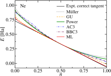
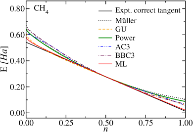
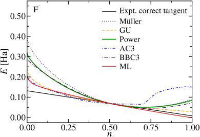
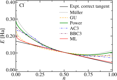
Figure 1: (Color online) The total energy, $E$, as a function of the occupation number, $n$, of the HOMO, for Ne atom and CH₄ (top) and the negative ions F^- and Cl^- (bottom). The line giving the correct experimental values for IP/EA is also shown. Curves are shifted to coincide at $n=1/2$ in order to compare the tangents with the straight line reproducing the experimental results. The values at the two ends are used in DIF for the calculation of IP for Ne, CH₄ and the affinity of F, Cl. The derivatives at $n=1/2$ are used for the calculation of the same quantities with the DER method.

We calculate the IPs and EAs of a set of atoms and molecules using DEF, DIF, and DER methods [i.e., using the Eqs. (4), (5) and (6)]. For comparison, results are also calculated using the EKT method. Our implementation is included in a computer code for finite systemscod which minimizes 1-RDM functionals with respect to occupation numbers and natural orbitals and is based on the expansion of the orbitals in Gaussian basis sets. The one- and two-electron integrals are calculated by use of the GAMESS programSchmidt et al. (1993). Addition or removal of an electron requires the extension of the theory to open shells. In the present work, like in Refs. [Helbig et al., 2007, 2009; Lathiotakis et al., 2010b; Helbig et al., 2011] we use the simple extension proposed in Ref. [Lathiotakis et al., 2005]. In other words, we assume that orbitals are spin independent while occupation numbers are spin dependent.

For the calculation of IPs we adopt the cc-pVDZ basis setT. H. Dunning, Jr. (1989) for all elements. EAs are calculated as the IPs of negative ions, i.e., of $N+1$ electrons. In other words, for both IPs and EAs, the orbital energy of the HOMO (for either the neutral or ionic system) is calculated. Since the HOMOs of the negative ions are relatively diffuse states, the aug-cc-pVDZ basis set is used T. H. Dunning, Jr. (1989). We should mention that a lot of neutral systems do not bind an extra electron. In that case, EA is equal to zero, i.e. the extra electron is completely delocalized. However, for small positive EA, the state of the extra electron can be delocalized and impossible to describe with localized basis sets. To ensure fair comparison with experiments a set of atoms, molecules and radicals which are known experimentally to have relatively large and positive EA is used.

Calculation of IPs and EAs with DEF method requires the difference of two energies, one for a closed-shell and another for an open shell-system. The broken spin symmetry in open-shell systems leads to twice as many variational parameters as there are in a closed shell system. This extra variational freedom over correlates the open-shell systems leading to systematic errors in IPs and EAs. Given the exact xc functional the DEF method would be exact, however, for an approximate functional the DEF method would show these systematic errors in IPs and EAs. DIF and DER methods on the other hand do not suffer from this error since only one minimization, for the charge neutral system, is performed. In addition, it should not come as a surprise if the DER method performs better than DEF and DIF in many cases as it suffers less from possible inaccuracies introduced by the functional and its non unique extension to the case of open shells, mainly because only the $1/2$ electron is present in the open shell. One could also consider DER method in conjunction with orbital relaxation (at fixed $n_{j}=1/2$). However, this procedure requires full orbital minimization for each $j$ making it computationally very demanding, while the aim of the present work is to define a computationally inexpensive single electron spectrum in terms of the optimal 1RDM of the charge neutral system.

Functional	$\bf\Delta_{\rm DEF}$(%)	$\bf\Delta_{\rm DIF}$(%)	$\bf\Delta_{\rm DER}$(%)
Müller	69.85	88.55	63.24
GU	44.91	65.96	70.81
Power	64.69	63.57	48.73
AC3	42.40	31.17	21.39
PNOF1	39.68	61.44	28.63
BBC3	30.00	55.33	52.00
ML	39.32	47.81	21.53
HF	55.00
CI/QCI(T)	17.28

Table 3: Average absolute errors $\Delta_{\rm DEF}$, $\Delta_{\rm DIF}$, and $\Delta_{\rm DER}$, in the calculation of EAs for a set of atoms, molecules and radicals calculated with various xc functionals using DEF, DIF, and DER respectively.

Another point to be considered is that the application of the DER method requires the total energy functional to be continuous at $n_{k}=1/2$. However, there are functionals that introduce a discontinuity at $n_{k}=1/2$ to distinguish between strongly and weakly occupied orbitalsLeiva and Piris (2006). In all cases studied here, we do not find optimal occupation numbers equal to 1/2. Thus, the step function can be safely shifted slightly away from $n_{k}=1/2$ without affecting the results. However, this procedure cannot be used in cases with optimal occupations equal to 1/2, like H₂ at the dissociation limit or when they vary continuously from 1 to zero.

System	Müller	GU	Power	AC3	PNOF1	BBC3	ML	QCI(T)	Expt.
LiH	0	0.192	0	0.219	0.317	0.106	0.264	0.317	0.34
OH	3.157	6.735	3.456	2.626	1.784	3.157	2.441	1.645	1.83
F	5.651	3.297	5.040	3.196	3.552	5.539	4.363	3.241	3.34
Li	0	0.403	0.139	0.275	0.400	0	0.212	0.601	0.62
Cl	3.687	2.190	3.632	3.678	2.660	4.186	3.623	3.430	3.61
CN	1.807	2.328	2.332	4.264	2.470	4.873	4.585	3.627	3.77
C2	1.044	1.419	1.298	3.386	4.416	4.560	3.722	3.055	3.54
BO	1.243	1.326	1.982	3.252	2.076	3.222	3.252	2.359	2.83
SH	1.386	0.706	1.908	1.968	1.352	2.454	2.168	2.119	2.32
PH	0.304	0	1.200	1.252	0.186	2.192	1.145	2.023	1.00
$\bf\Delta$(%)	63.24	70.81	48.73	21.39	28.63	52.00	21.53	17.28

Table 4: Electron Affinities for various atoms, molecules and radicals calculated as the IP of the system of $N+1$ electrons with different functionals using the DER method. For systems where $N+1$ electrons energy is found higher than the $N$ electron energy, zero affinity is assumed. The results are compared with QCI(T) and experiments. QCI(T) values were calculated with Gaussian 09 programFrisch et al. .

IV results

Our results for the average absolute errors in the calculation of IPs with the three methods are included in Table 1. Average errors in the results obtained with EKT method are also included in the table. The actual values for IPs obtained using the DER method are compiled in Table 2. (Full results for all methods as well as EKT can be found in the supplementary materialsup .) It is clear from Table 1 that all functionals in combination with the DER method give reasonable results for IPs with errors ranging from 4 to 13%. ML, AC3 and power functionals perform slightly better by giving an average error of only 4-6%. For the systems considered here, the ML functional with the DER method is the most accurate for the FIPs (with an error of only 2%). It is important to note that the errors from the DER and EKT method are of the same order (using the same functionals and basis set), while there is less computational effort involved in DER method. The comparison of the DIF and DER methods allows us to assess the validity of the linear approximation–the linearity of the total energy with respect to variation of one occupation number while keeping the rest of the occupation numbers as well as natural orbitals frozen (this was demonstrated for solids in Ref. [Sharma et al., 2009]). As we see in Table 2, the DER method gives good results also for finite systems and for the best performing functionals the average difference between the DIF and DER methods’ results is in the range of 2-7%. This percentage may be regarded as the magnitude of non-linearity of the total energy with respect to variation of a single occupation number.

As mentioned in Sec. III, the DEF method suffers from the over correlation error due to the approximate nature of the xc functional and the difference in variational freedom between closed and open-shell systems. Since the DER method is less prone to this error, it is not a surprise that for the power and ML functionals the DER method improves the results over the DEF method. This indicates that the dependence of the total energy on a particular occupation number deviates from linearity but this deviation works in favor of the DER method by further improving the results. In order to understand this, in Fig. 1(top), we show the tangents at 1/2 of the total energy as a function of the occupation number of the HOMO, while keeping the rest frozen. The plots are made for various functionals. It is clear from Fig. 1 that although the total energy functional itself deviates from linearity the tangent at 1/2 is very close to the one that reproduces the experimental results. One reason for this improvement over the DIF method might be that the extension of the theory to open shells in the case the DER method is minimal– since only half of an electron is unpaired– and DER method reduces the error introduced by the extension of functionals to open shells.

The average percentage errors and the values of HIPs for various atoms and molecules are also presented in Table 1 and Table 2 respectively. The average error in HIPs obtained using the Müller, GU, power and PNOF1 functionals, is substantially lower (4-7%) than for the FIPs. The rest of the functionals are less accurate for HIPs with average absolute errors slightly higher than those for the FIPs (5-10%).

The average absolute errors in the calculation of EAs with the DEF, DIF, and DER methods are shown in Table 3. The actual values for EAs obtained using DER method are included in Table 4. As already mentioned, EAs are more difficult quantities to calculate– the errors are introduced by describing negative ions with localized basis which are usually optimized for the description of the ground states of neutral systems. In addition, being a small quantity, EAs are more prone to errors in the differences of total energies corresponding to two different shell structures (for example the difference in energy between a doublet and a singlet state). Thus, it is not surprising that the errors in Tables 3 and  4 are substantially higher than for the IPs. However, state-of-the art quantum chemical methods like QCI(T) also exhibit large errors within the adopted basis set. Under these considerations the AC3, PNOF1 and ML functionals perform surprisingly well for EAs with average errors of 21.4%, 28.6%, and 21.5% respectively. These errors are close to that of QCI(T) (17.3%). It is interesting to note that (see Table 4) there are only a few cases (5 of 60) for which Müller, GU, BBC3 and power functionals give a zero EA [$E(N+1)>E(N)$], i.e., the system is not predicted by the corresponding functional to bind an extra electron. For the best performers like the AC3, PNOF1, and ML functionals, no such case exists.

In order to compare the DIF and DER methods for the determination of EAs, Fig. 1(bottom) shows the tangents at 1/2 to the dependence of the total energy on the occupation of the HOMO of the negative ions F^- and Cl^-. The exact tangent that reproduces the experimental EAs is also shown in the figure. Again, as in the case of IPs, the DER method not only looks like a reasonable approximation but it also improves on the results of the DEF method (for the functionals considered and in all cases studied in the present work). In particular, for the case of Cl^- [see Fig. 1(bottom)] the tangents at 1/2 are in very good agreement with the exact tangent that reproduces experimental EA, although the dependence of the total energy on the HOMO occupation number deviates significantly from linearity.

A striking example of the pathological behavior mentioned in Sec. III is the negative ion F^-. This system is found experimentally to be energetically lower than the neutral F atom by 3.34 eV (see Table  4). All functionals underestimate this energy substantially (see supplementary material sup ), as a result of the enhanced variational freedom of the open-shell, neutral F atom compared to the closed-shell F^-. In two extreme cases (ML and AC3 functionals) F^- is found energetically above the neutral F atom.

V summary

In summary we examined the performance of the derivative-method proposed in Ref. [Sharma et al., 2009] for calculation of the IPs and EAs of finite systems. The accuracy of IPs and EAs calculated using the derivative-method are compared to the IPs and EAs calculated using the definition of these quantities [which involves two total energy minimizations for the system and the positive (for IP) or negative ion (for EA)]. In order to have a complete analysis we have also considered an intermediate method (difference method), in which the IPs and EAs are determined by the difference of the total energies with fixing one occupation number to 1 and/or zero. All these results are further compared to the state-of-the-art CI method as well as experiments.

We find that, for IPs both the difference and derivative methods are good approximations to the definition of this quantity. Furthermore, it was found that the derivative method results, obtained using Müller, power, and ML functionals, are better than the values obtained using the definition method itself (with errors of the order of 4-8% only). Among these functionals the ML functional in conjunction with derivative method is most accurate with errors of only up to 2%. For the EAs the errors are significantly larger, with the ML functional in conjunction with the derivative method being the most accurate (with an error of 21%). The errors in EAs were found to be comparable to the errors in the CI results.

From the present study we conclude that the results of the derivative method for IPs and EAs are in good agreement with experiments and this method is a promising technique to obtain the single-electron spectrum for systems where state-of-the-art quantum chemical methods can not be applied and DFT results deviate significantly from experiment.

References

- Godby et al. (1986) R. W. Godby, L. J. Sham, and M. Schlüter, Phys. Rev. Lett. 56, 2415 (1986).
- Sharma et al. (2008) S. Sharma, J. K. Dewhurst, N. N. Lathiotakis, and E. K. U. Gross, Phys. Rev. B 78, 201103 (2008).
- Coleman (1963) A. Coleman, Rev. Mod. Phys. 35, 668 (1963).
- Buijse and Baerends (2002) M. A. Buijse and E. J. Baerends, Mol. Phys. 100, 401 (2002).
- Müller (1984) A. M. K. Müller, Phys. Lett. 105A, 446 (1984).
- Staroverov and Scuseria (2002) V. N. Staroverov and G. E. Scuseria, J. Chem. Phys. 117, 2489 (2002).
- Herbert and Harriman (2003) J. M. Herbert and J. E. Harriman, Chem. Phys. Lett. 382, 142 (2003).
- Gritsenko et al. (2005) O. Gritsenko, K. Pernal, and E. J. Baerends, J. Chem. Phys. 122, 204102 (2005).
- Frank et al. (2007) R. L. Frank, E. H. Lieb, R. Seiringer, and H. Siedentop, Phys. Rev. A 76, 052517 (2007).
- Lathiotakis et al. (2007) N. N. Lathiotakis, N. Helbig, and E. K. U. Gross, Phys. Rev. B 75, 195120 (2007).
- Goedecker and Umrigar (1998) S. Goedecker and C. J. Umrigar, Phys. Rev. Lett. 81, 866 (1998).
- Lathiotakis et al. (2005) N. N. Lathiotakis, N. Helbig, and E. K. U. Gross, Phys. Rev. A 72, 030501 (2005).
- Piris (2006) M. Piris, Int. J. Quant. Chem 106, 1093 (2006).
- Leiva and Piris (2005) P. Leiva and M. Piris, J. Chem. Phys. 123, 214102 (2005).
- Leiva and Piris (2007) P. Leiva and M. Piris, Int. J. Quant. Chem. 107, 1 (2007).
- Helbig et al. (2007) N. Helbig, N. N. Lathiotakis, M. Albrecht, and E. K. U. Gross, Europhys. Lett. 77, 67003 (2007).
- Pernal (2005) K. Pernal, Phys. Rev. Lett. 94, 233002 (2005).
- Lathiotakis and Marques (2008) N. N. Lathiotakis and M. A. L. Marques, J. Chem. Phys. 128, 184103 (2008).
- Marques and Lathiotakis (2008) M. A. L. Marques and N. N. Lathiotakis, Phys. Rev. A 77, 032509 (2008).
- Requist and Pankratov (2008) R. Requist and O. Pankratov, Phys. Rev. B 77, 235121 (2008).
- Piris et al. (2009) M. Piris, J. Matxain, and X. Lopez, J. Chem. Phys. 131, 021102 (2009).
- Rohr et al. (2008) D. R. Rohr, K. Pernal, O. V. Gritsenko, and E. J. Baerends, J. Chem. Phys. 129, 164105 (2008).
- Lathiotakis et al. (2009a) N. N. Lathiotakis, N. Helbig, A. Zacarias, and E. K. U. Gross, J. Chem. Phys. 130, 064109 (2009a).
- Piris et al. (2010) M. Piris, J. M. Matxain, X. Lopez, and J. M. Ugalde, J. Chem. Phys. 132, 031103 (2010).
- Eich et al. (2010) F. G. Eich, S. Kurth, C. R. Proetto, S. Sharma, and E. K. U. Gross, Phys. Rev. B 81, 024430 (2010).
- Lathiotakis et al. (2010a) N. N. Lathiotakis, N. I. Gidopoulos, and N. Helbig, J. Chem. Phys. 132, 084105 (2010a).
- Tolo and Harju (2010) E. Tölö and A. Harju, Phys. Rev. B 81, 075321 (2010).
- Rohr et al. (2010) D. R. Rohr, J. Toulouse, and K. Pernal, Phys. Rev. A 82, 052502 (2010).
- Piris et al. (2011) M. Piris, X. Lopez, F. Ruipérez, J. M. Matxain, and J. M. Ugalde, J. Chem. Phys. 134, 164102 (2011).
- Helbig et al. (2009) N. Helbig, N. N. Lathiotakis, and E. K. U. Gross, Phys. Rev. A 79, 022504 (2009).
- Lathiotakis et al. (2010b) N. N. Lathiotakis, S. Sharma, N. Helbig, J. K. Dewhurst, M. A. L. Marques, F. Eich, T. Baldsiefen, A. Zacarias, and E. K. U. Gross, Zeitschrift für Physikalische Chemie 224, 467 (2010b).
- Lathiotakis et al. (2009b) N. N. Lathiotakis, S. Sharma, J. K. Dewhurst, F. G. Eich, M. A. L. Marques, and E. K. U. Gross, Phys. Rev. A 79, 040501 (2009b).
- Pernal and Cioslowski (2005) K. Pernal and J. Cioslowski, Chem. Phys. Lett. 412, 71 (2005).
- Leiva and Piris (2006) P. Leiva and M. Piris, Journal of Molecular Structure:THEOCHEM 770, 45 (2006).
- Sharma et al. (2009) S. Sharma, S. Shallcross, J. K. Dewhurst, and E. K. U. Gross, http://www.arxiv.org, cond-mat: arXiv:0912.1118 (2009).
- Curtiss et al. (1998) L. A. Curtiss, P. C. Redfern, K. Raghavachari, and J. A. Pople, J. Chem. Phys. 109, 42 (1998).
- McCormack et al. (1989) E. McCormack, J. M. Gilligan, C. Cornaggia, and E. E. Eyler, Phys. Rev. A 39, 2260 (1989).
- Ihle and Wu (1975) H. R. Ihle and C. H. Wu, J. Chem. Phys. 63, 1605 (1975).
- Bahr et al. (1969) J. L. Bahr, A. J. Blake, J. H. Carver, and V. Kumar, J.Quant.Spectrosc.Radiat.Transfer. 9, 1359 (1969).
- Cederbaum and von Niessen (1974) L. S. Cederbaum and W. von Niessen, Chem. Phys. Lett. 24, 263 (1974).
- Bieri and Asbrink (1980) G. Bieri and L. Asbrink, Journal of Electron Spectroscopy and Related Phenomena 20, 149 (1980).
- (42) M. J. Frisch, G. W. Trucks, H. B. Schlegel, G. E. Scuseria, M. A. Robb, J. R. Cheeseman, G. Scalmani, V. Barone, B. Mennucci, G. A. Petersson, et al., Gaussian 09 Revision A.1, gaussian Inc. Wallingford CT 2009.
- Janak (1978) J. F. Janak, Phys. Rev. B 18, 7165 (1978).
- (44) HIPPO computer program, info: lathiot@eie.gr.
- Schmidt et al. (1993) M. W. Schmidt, K. K. Baldridge, J. A. Boatz, S. T. Elbert, M. S. Gordon, J. H. Jensen, S. Koseki, N. Matsunaga, K. A. Nguyen, S. J. Su, et al., J. Comp. Chem. 14, 1347 (1993).
- Helbig et al. (2011) N. Helbig, G. Theodorakopoulos, and N. N. Lathiotakis, J. Chem. Phys. 135, 054109 (2011).
- T. H. Dunning, Jr. (1989) T. H. Dunning, Jr., J. Chem. Phys. 90, 1007 (1989).
- Sarkas et al. (1994) H. W. Sarkas, J. H. Hendricks, S. T. Arnold, and K. H. Bowen, J. Chem. Phys. 100, 1884 (1994).
- Meunier et al. (1999) M. Meunier, N. Quirke, and D. Binesti, Molecular Simulation 23, 109 (1999).
- (50) See supplementary material at [URL will be inserted by AIP] for a set of tables containing our calculation results for the IPs and EAs using RDMFT functionals with methods DEF, DIF, and DER, as well as extended Koopman’s theorem.