Rectification of THz-radiation in semiconductor superlattices in the absence of domains

Abstract

We study theoretically the dynamical rectification of a terahertz ac electric field, i.e. the dc current and voltage response to the incident radiation, in strongly coupled semiconductor superlattices. We address the problem of stability against electric field domains: A spontaneous dc voltage is known to appear exactly for parameters for which a spatially homogeneous electron distribution is unstable. We show that by applying a weak direct current bias the rectifier can be switched from a zero dc voltage state to one with a finite voltage in full absence of domains. The switching occurs near the conditions of dynamical symmetry breaking of an unbiased semiconductor superlattice. Therefore our scheme allows for the generation of dc voltages that would otherwise be unreachable due to domain instabilities. Furthermore, for realistic, highly doped wide miniband superlattices at room temperature the generated dc field can be nearly quantized, that is, be approximately proportional to an integer multiple of $\hbar\omega/ea$ where $a$ is the superlattice period and $\omega$ is the ac field frequency.

1 Introduction

Semiconductor superlattices (ssls) have been the subject of much research ever since Esaki and Tsu[1] realized that these nanostructures could exhibit Bloch-oscillations[2] at moderate electric field strengths. This oscillatory response makes ssls inherently nonlinear, and the variety of transport phenomena that has been discovered has lead to the point that they can now be called model systems for nonlinear transport[3]. Semiconductor superlattices hold great promise as amplifiers and detectors of THz radiation. A considerable amount of research has been put into the problem of THz gain with promising findings both in theory[4, 5, 6] and in experiments[7, 8, 9]. Quantum direct detection[10, 11, 12] by THz photon induced reduction in current has been experimentally observed[13, 14, 15] and then applied to ultrafast detection and autocorrelation of short THz pulses[16, *winnerl99]. A further topic on ssls is strongly nonlinear dynamical phenomena that arise if one considers for example circuit models of ssl devices that incorporate effects that come from the interaction of the charge carriers. This gives rise to novel effects such as dissipative chaos[18, 19], and spontaneous generation of quantized [20, 21, 22, 23, 24], fractionally quantized, and non-quantized[23, 25] dc bias. This spontaneous generation of a dc field is also the topic of this paper.

Spontaneous generation of dc bias is the dynamical effect whereby a direct electric field appears due to a pure ac excitation. A significant point is that this spontaneous dc bias can in ssls be nearly quantized, meaning that the total dc electric field, $E_{\mathrm{dc}}$ follows the relationship

$$E_{\mathrm{dc}}=\eta n\frac{\hbar\omega}{ae},$$ (1)

where $n$ is an integer, $\omega$ is the frequency of the incident radiation field and the coefficient $\eta$ represents the fractional deviation from perfect quantization, $\eta=1$. The remaining constants are $a$, $\hbar$, and $e$, which are the superlattice period, the reduced Planck constant, and the electron charge, respectively. This phenomena bears close resemblance to the inverse ac-Josephson effect[26, 27], and is in fact just one example of similarity between Josephson junctions and ssls[28, 19, 29]. Unquantized spontaneous dc has also been predicted for lateral semiconductor superlattices[30, 29] that only differ by their geometry from the bulk ssls studied here. Similar effect has been earlier described in some models of homogeneous bulk semiconductors[31, *bumyalene89-trans].

We emphasize that this type of rectification occurs in perfectly symmetric structures, unlike classical rectification that relies on transport asymmetry due to contact charge inhomogeneities or nonlinearity. Rather, here a static dc field is formed dynamically due to presence of absolute negative conductivity (anc) at zero dc bias[20, 21]. anc in itself, is a well-known effect in ssls[33, *pavlovich76nt, 35, 36], and has been theoretically found to be a robust effect in ssls, occurring for a variety of miniband dispersions[37] and external excitations[38, 39, 40].

In ssls the relationship (1) can persist for a wide range of parameters and so this effect suggest the use of them as new type of frequency-to-voltage converters. A major hurdle exists, however, in the practical application of rectification in ssls: The parameters for which this dynamical rectification is expected to happen overlap exactly with the regions where the homogeneous spatial charge distribution is unstable. In this paper, we explore a possible way of avoiding this problem, and show that it should indeed be possible to observe the generation of a nearly quantized dc field with realistic ssl parameters.

2 Effective circuit model with a dc current source

As our model, we use an effective circuit calculation similar to [11, 41, 23] where the active part, the ssl, is connected to an ac circuit modeling an antenna that couples the radiation field to the device. A schematic figure of the setup is presented in figure 1. The external electric field generates an oscillating contribution $U_{\mathrm{ext}}=U_{1}\cos\omega t$ to the total potential across the device: $U=U_{\mathrm{ext}}-\ell E$, where $E$ is the electric field in the active region and $\ell$ is its length. We take the amplitude $U_{1}$ and frequency $\omega$ of the external potential as our given parameters. Contributions from displacement currents are taken into account. Our new idea is to include a circuit that acts as a direct current source, providing a fixed current $I_{\mathrm{dc}}$. The dc voltage will then be determined by a self-consistent calculation of the model equations. We consider this voltage as the output of the device.

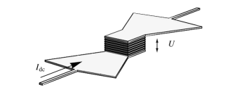
Figure 1: Schematic figure of the ssl rectifier and the antenna. Incident radiation creates an oscillating potential $U_{\mathrm{ext}}$ and a fixed current $I_{\mathrm{dc}}$ is supplied via the leads connected to the antenna.

The active part of the THz-rectifier is modeled using the well-known superlattice balance equations for sinusoidal miniband[3, 21]:

$$\dot{V} = -\frac{ea^{2}E}{\hbar^{2}}\left(W-\frac{\Delta}{2}\right)-\frac{1}{\tau_{\mathrm{v}}}V,$$ (2a)

$$\dot{W} = eEV-\frac{1}{\tau_{\mathrm{w}}}(W-{W_{\mathrm{eq}}}).$$ (2b)

The variables $V$ and $W$ are the average electron velocity and energy, respectively, where the averaging is done over a distribution function obeying the Boltzmann transport equation. ${W_{\mathrm{eq}}}$ is the equilibrium energy, ${W_{\mathrm{eq}}}=-(\Delta/2)I_{1}(\Delta/(2k_{\mathrm{b}}T))/I_{0}(\Delta/(2k_{\mathrm{b}}T))$, where $\Delta$ is the miniband width, $T$ temperature, $k_{\mathrm{b}}$ Boltzmann constant, and $I_{0,1}$ are modified Bessel functions. $E(t)$ is the total electric field that the miniband electrons experience, and it is obtained using the equation for current continuity across the active part of ssl:

$$\frac{\varepsilon_{0}}{4\pi}\dot{E}+j+\frac{\ell}{AR}E=j_{\mathrm{ext}}.$$ (3)

Above, $\varepsilon_{0}$ is the average dc dielectric constant of the superlattice, $j$ is the conduction electron current density across the superlattice, $R$ is a resistance that models ohmic losses in the superlattice, $A$ is the area of superlattice cross section, and $j_{\mathrm{ext}}$ is the external current density. This in turn is determined by considering the effective circuit model, which gives $Aj_{\mathrm{ext}}=C_{\mathrm{a}}\dot{U}+I_{\mathrm{dc}}$ with $C_{\mathrm{a}}$ being an effective antenna capacitance. The current density $j$ is given by $j=enV$, where $n$ is the electron density of the superlattice. Together, (2) and (3) give a closed set of first order nonlinear ordinary differential equations.

To facilitate analysis, we scale the variables $V$ and $W$ by their maximum values, giving $W=(\Delta/2)(1+w)$, $V=a\Delta(2\hbar)^{-1}\,v$. The new variables, scaled electron velocity and energy, $v$ and $w$ have the range $-1\ldots+1$. Electric fields are converted to frequency units by multiplying by $ea/\hbar$: $eaE/\hbar=u$. We obtain

$$\dot{v} = -uw-\gamma_{\mathrm{v}}v,$$ (4a)

$$\dot{w} = \phantom{-}uv-\gamma_{\mathrm{w}}(w-w_{\mathrm{eq}}),$$ (4b)

$$\dot{u} = -r^{2}v-\alpha u+{\dot{\phi}}_{\mathrm{ext}},$$ (4c)

$$\phi_{\mathrm{ext}} = \omega_{\mathrm{s}}\cos\omega t+i_{0}t,$$ (4d)

where $r^{2}=\omega_{\mathrm{pl}}^{2}/(1+C_{\mathrm{a}}/C_{\mathrm{s}})$, the drive amplitude $\omega_{\mathrm{s}}=eaU_{1}/(\hbar\ell(1+C_{\mathrm{s}}/C_{\mathrm{a}}))$, the electric field damping $\alpha=R^{-1}(C_{\mathrm{s}}+C_{\mathrm{a}})^{-1}$, the current bias $i_{0}=aeI_{\mathrm{dc}}/(\hbar\ell(C_{\mathrm{s}}+C_{\mathrm{a}}))$, the superlattice capacitance $C_{\mathrm{s}}=\varepsilon_{0}A/(4\pi\ell)$ and

$$\omega_{\mathrm{pl}}^{2}=\frac{2\pi e^{2}na^{2}\Delta}{\hbar^{2}\varepsilon_{0}}.$$ (5)

Here, $\omega_{\mathrm{pl}}$ is the plasma frequency and it describes the free oscillation frequency of the electron gas, and also serves as the parameter that determines the amount of nonlinearity. Note, that excluding the dc bias current term, equations (4) are formally equivalent to those used in [18, 22]. For our simulations we use parameter values that closely match those of the superlattice studied in [42]: $\Delta=120\;{\mbox{meV}}$, superlattice period $a=46\;{\mbox{\AA}}$, number of layers $N=130$, $n=9\cdot 10^{17}\;{\mbox{cm}}^{-3}$, $\gamma_{\mathrm{v}}=15\;{\mbox{THz}}$, $\gamma_{\mathrm{w}}=3\;{\mbox{THz}}$, and temperature $T=300\;{\mbox{K}}$. In addition we choose $C_{\mathrm{a}}=C_{\mathrm{s}}\simeq 5\;{\mbox{fF}}$, $R=1\;{\mbox{k$\Omega$}}$, roughly matching values used in [23]. Denoting $\tau=1/\sqrt{\gamma_{\mathrm{v}}\gamma_{\mathrm{w}}}$, the above values give $r\tau\simeq 2.25$, $\alpha\tau\simeq 0.015$, and $w_{\mathrm{eq}}\simeq-0.75$.

In this paper we then consider the dc part $u_{0}$ of the total electric field $u$, $u_{0}=\langle u\rangle$. We would like to find spontaneous generation of dc bias, i.e. $\langle u\rangle\neq 0$, preferably nearly quantized so that $\langle u\rangle\simeq n\omega$. In the absence of the dc drive current, (4) remains invariant in the transformation $\mathcal{S}$:

$$(t,v,w,u)\stackrel{{\scriptstyle\mathcal{S}}}{{\to}}(t+T/2,-v,w,-u),$$ (6)

where $T=2\pi/\omega$ is the period of the external ac field. If the governing equations remain invariant in transformation $\mathcal{S}$, we say that they are symmetric or have symmetry $\mathcal{S}$. In our previous works we have focused on the appearance of a spontaneous dc voltage via dynamical symmetry breaking[22, 19, 30, 43, 29]. Let $u_{0}$ be the generated dc voltage: $u_{0}=\langle u\rangle=T^{-1}\int_{0}^{T}u(t^{\prime})\;\mathrm{d}t^{\prime}$ (we use $\langle\cdot\rangle$ to denote time averages over the period of the function being averaged). If the equations have symmetry $\mathcal{S}$, a state with a nonzero average voltage, $u_{0}\neq 0$, implies that the solutions themselves do not follow symmetry $\mathcal{S}$: $(v(t+T/2),w(t+T/2),u(t+T/2))\neq(-v(t),w(t),-u(t))$. This is dynamical symmetry breaking. Here however, symmetry $\mathcal{S}$ is not present in the equations if $i_{0}\neq 0$, and therefore one cannot speak of spontaneous dc following the breaking of symmetry. In spite of this, we will show that a key feature of spontaneous generation of a dc field remains: a sharp change in the total dc field near the conditions of symmetry breaking and also the quantization of that dc component. It should be noted that the dc bias current will only be essential during the turn-on of the device. Nothing prohibits disconnecting the bias current and restoring the symmetry of the problem after the device has settled to a steady state.

The present work specifically addresses the problem of domain instabilities. An underlying assumption in the models used to predict the spontaneous dc field is that the electron distribution is spatially homogeneous. It is, however, well known that in the presence of negative differential conductivity (ndc), the homogeneity of the distribution tends to be violated and domains of different electric field strengths form[44, 45, *ktitorov-trans, 47]. This issue has been mainly ignored in previous works. For stable operation of the device as a THz-rectifier we then require that

$$\frac{\partial v_{\mathrm{dc}}}{\partial u_{\mathrm{dc}}}>0,$$ (7)

where $v_{\mathrm{dc}}=\langle v\rangle$ is the current averaged over its temporal period and $u_{\mathrm{dc}}$ is a dc probe field introduced to the total field $u$: $u\to u+u_{\mathrm{dc}}$. We will refer to the steady state values of the realized dc electric field and current as the operating point.

Condition (7) also effectively determines the appearance of a spontaneous dc field. Suppose $\bar{v},\bar{w}$ is a solution to the two first equations of (4) for a given field $\bar{u}$ containing a dc probe field represented by a slow function $u_{\mathrm{dc}}$. Substituting to (4c) one gets ${\dot{u}}_{\mathrm{dc}}=-r^{2}\langle\bar{v}\rangle(u_{\mathrm{dc}})-\alpha u_{\mathrm{dc}}$. An equilibrium value of $u_{\mathrm{dc}}$ is stable if the derivative of the right-hand side with respect to $u_{\mathrm{dc}}$ is negative:

$$-r^{2}\frac{\partial\langle\bar{v}\rangle}{\partial u_{\mathrm{dc}}}(u_{\mathrm{dc}})-\alpha<0.$$ (8)

Above, $\langle\bar{v}\rangle$ is the time average of $\bar{v}$, which is simply the dc current. Presence of the electric field damping $\alpha$ has the effect of stabilizing the dc field, however in the $\alpha\to 0$ limit equations (8) and (7) coincide. Therefore, in order to achieve spontaneous dc from pure ac excitation, the superlattice needs to be driven into ndc. In the following sections, however, we will show that a small dc bias current can make the current-voltage curve (iv-curve) slope positive across a range of parameters while at the same time allowing for a substantial dc voltage to appear.

As the final point regarding stability against domains, we note that we should strengthen condition of (7). In an experimental setup the external ac field does not rise instantly, and so during turn-on and the initial transient phase the device might not be stable against domains. In the absence of a model that would take into account both formation of domains and spontaneous dc, we resort to comparing characteristic time scales for both processes to estimate which will dominate. Switching times $\tau_{\mathrm{sw}}$, that is, the time it takes for a spontaneous dc to appear should be faster than the domain formation times $\tau_{\mathrm{dom}}$ to avoid the interference of the domains. In [21] where a similar model of a ssl rectifier was used, $\tau_{\mathrm{sw}}$ was calculated to be at least in the range of hundreds of ac drive cycles $T=2\pi/\omega$ in the case of heavily doped wide miniband superlattices. On the other hand, for similar superlattices the domain formation times can be as short as fractions of picoseconds[48]. Both of these characteristic times scale down as $\omega_{\mathrm{pl}}$ is increased, and since it is the dressed plasma frequency $r$, $r<\omega_{\mathrm{pl}}$, that here determines the switching time, we may suppose that $\tau_{\mathrm{dom}}\lesssim\tau_{\mathrm{sw}}$. This suggests that domains are likely to occur instead of spontaneous dc. This problem of ndc during turn-on and transient can be solved by assuming that the external potential is turned on slowly, and requiring that the device is stable for all drive amplitudes below the intended target value. This additional criterion bypasses all the uncertainty related to transients and should guarantee us stable operation. Next, we will show that in the limit $\omega_{\mathrm{pl}}\tau\lesssim 1$ these requirements cannot be satisfied if a pure ac drive is considered, but can be if a small dc bias current is introduced.

3 Weak DC biased switching in the $\omega_{\mathrm{pl}}\tau\ll 1$ limit

First, let us consider the case where we only include the first harmonic of the field $u$. We assume the electric field has the form $u=u_{0}+u_{1}\cos\omega t$, and neglect the dependence of $u_{1}$ on our main parameters $\omega_{\mathrm{s}}$ and $\omega$. Also, we set $\gamma_{\mathrm{v}}=\gamma_{\mathrm{w}}=\gamma$. The first harmonic approximation is valid when the nonlinearity is weak, that is, when $\omega_{\mathrm{pl}}\tau\ll 1$.

Consider the dc part of the total electric field $u$. Averaging (4c) yields

$$r^{2}v_{0}(u_{0},u_{1},\omega)=-\alpha u_{0}+i_{0},$$ (9)

where $v_{0}(u_{0},u_{1},\omega)$ is the dc current under ac field $u_{1}\cos\omega t$. The resulting net voltage and the corresponding current are found at the intersection of the iv-curve and the line $v_{\mathrm{r}}$,

$$v_{\mathrm{r}}(u_{0})=r^{-2}(-\alpha u_{0}+i_{0}).$$ (10)

For a given electric field $u$, $v_{0}(u_{0},u_{1},\omega)$ can be explicitly written out as[3, 49]

$$v_{0}(u_{0},u_{1},\omega)=\sum_{n=-\infty}^{\infty}J^{2}_{n}\left(\frac{u_{1}}{\omega}\right)v_{\mathrm{ET}}(u_{0}+n\omega),$$ (11)

$$v_{\mathrm{ET}}(u)=|w_{\mathrm{eq}}|\frac{\gamma u}{\gamma^{2}+u^{2}}.$$ (12)

The dependence $v_{\mathrm{ET}}(u)$ is the Esaki-Tsu current voltage curve [1] and in (11) we see the familiar form of an ac irradiated superlattice where the $n$th term represents an $n$-photon-assisted replica of $v_{\mathrm{ET}}$[3, 50, 51].

The effect of the dc bias is to shift the operating point to high dc field values as the ac amplitude is increased. This can be seen by considering a small dc voltage $u_{0}$. Expanding (11) to leading order in $u_{0}$ gives

$$v_{0}(u_{0},u_{1},\omega)\simeq g_{0}(u_{1},\omega)u_{0},$$ (13)

where $g_{0}$ is the weak dc field conductivity of the ssl under dc and ac drives

$$g_{0}(u_{1},\omega)=\sum_{n=-\infty}^{\infty}J^{2}_{n}\left(\frac{u_{1}}{\omega}\right)v_{\mathrm{ET}}^{\prime}(n\omega)$$ (14)

and the prime symbol means the derivative with respect to $u$. In the weak dc field limit, stability condition (7) is equivalent to $g_{0}(u_{1},\omega)>0$. Therefore, we wish to see how $u_{0}$ changes as $g_{0}$ tends to zero. The generated voltage $u_{0}$ can be solved from (9):

$$u_{0}=\frac{i_{0}}{r^{2}g_{0}(u_{1},\omega)+\alpha}.$$ (15)

Setting $g_{0}$ to zero one finds that $u_{0}\to i_{0}/\alpha$, which is no longer a small quantity even for a relatively small $i_{0}$, since $\alpha\ll 1$. This suggests that before the onset of ndc, the net dc electric field tends to large values. This is the basis of the dc biased slow switching scheme that we propose: The dc bias results in a large generated dc field that appears before ndc, thus avoiding the domain instability where $g_{0}(u_{1},\omega)<0$. Clearly, this alone is not enough, since the actual realized operating point may in fact sit on the ndc part of the iv-curve. Whether or not this is the case will be determined by (7) and (9).

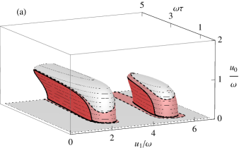
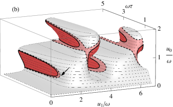
Figure 2: [Colour online] Generated dc voltage as a function of ac field amplitude $u_{1}$ and frequency $\omega$. Remaining parameters are $r\tau=1$, $\alpha\tau=0.015$, and $w_{\mathrm{eq}}=-0.75$. Regions shaded gray show stable operation. Dashed lines indicate borders of ndc [light red regions indicate ndc and domains], and solid thick lines show points of sn-bifurcations [dark red regions mark unstable branches of multistable operation]. Contours are plotted at level values of $u_{0}/\omega$ and are spaced at intervals of $0.1$. (a) Bias current off, $i_{0}=0$. Two regions of spontaneous dc are visible, however, they are flanked by regions unstable operation by all sides. (b) Bias current on, $i_{0}=i_{\mathrm{opt}}$. Strong response in $u_{0}$ is seen where spontaneous dc appeared in the unbiased case. Arrow at $u_{1}/\omega\approx 1.70$, $\omega\tau\approx 1.62$, $u_{0}/\omega\approx 0.39$ marks the point where ndc first appears. Stable operation with large $u_{0}$ is then possible for $\omega\tau\lesssim 1.6$.

Let us now consider the frequency dependence of $u_{0}$. In the high frequency $\omega\tau\gg 1$ limit the dc voltage can be very nearly quantized when the bias current is absent[21, 23]. This does not change when the dc drive is included. Since near $u_{0}=n\omega$ the $n$ photon term dominates the series expression (11), the current is approximately given by $J^{2}_{n}(u_{1}/\omega)v_{\mathrm{ET}}(u_{0}-n\omega)$. Using (9) and assuming $|u_{0}-n\omega|\ll 1$ we find that

$$u_{0}\simeq n\omega+\gamma\frac{i_{0}-\alpha n\omega}{\alpha\gamma+|w_{\mathrm{eq}}|J_{n}(u_{1}/\omega)^{2}r^{2}}.$$ (16)

The correction term is small since we take $i_{0}\tau^{2},\alpha\tau\ll 1$, and so the realized operating point voltage is nearly quantized. Further, this point is always stable provided $J_{n}(u_{1}/\omega)$ is not too close to zero. Note also, that (16) gives an approximate optimal drive current for observing quantized $u_{0}$. The correction term vanishes and the quantization is improved by choosing $i_{0}=i_{\mathrm{opt}}$ where

$$i_{\mathrm{opt}}=n\omega\alpha.$$ (17)

The high-frequency limit is also particularly susceptible to domain instabilities during turn-on. This is because of hysteretic response to changing drive amplitude. The current replicas, that is, the individual terms in (11), define local peaks in the iv-curve. Since the slope of $v_{\mathrm{r}}$ is low, the intersections between $v_{\mathrm{r}}$ and $v_{0}$ tend to come in pairs, one on each side of a local maximum of current. These intersections define a pair of operating points, one stable and the other unstable. Consider one such pair near $u_{0}=k\omega$. Should $J_{k}(u_{1}/\omega)$ tend to zero as $u_{1}$ increases, that local current peak dips below $v_{\mathrm{r}}$ and the operating points collide and are subsequently destroyed. This is essentially a saddle-node (sn) bifurcation and causes a problem since sn bifurcations always occur in conjunction with ndc. One can see this easily by noting that sn-bifurcation implies a double root of (9), which in turn means that slopes of $v_{0}$ and $v_{\mathrm{r}}$ must there agree:

$$\frac{\partial v_{\mathrm{dc}}}{\partial u_{\mathrm{dc}}}=-\frac{\alpha}{r^{2}}.$$ (18)

Clearly then, at an sn-bifurcation the system is already in ndc. Since equilibria are destroyed and created at sn-bifurcations, their presence implies multistability and hysteretic response. Requiring stability against formation of domains therefore means that the voltage $u_{0}$ response to changing $u_{1}$ must be non-hysteretic. This effectively sets an upper limit to the frequencies by which stable turn-on can be guaranteed.

In the low-frequency limit, $\omega\tau\ll 1$, the current adiabatically follows the unirradiated iv-curve (12). The dc current is then approximately given by $\langle v_{\mathrm{ET}}(u_{0}+u_{1}\cos\omega t)\rangle$. In this case, $u_{0}$ as given by (9) is always nearly zero, and exactly zero in the absence of the bias current. The low and high frequency limits together demonstrate that there is a band of frequencies near $\omega\tau\sim 1$ whereby strong response of $u_{0}$ can be observed without domains. In accordance with (16), the value of $u_{0}$ should be closest to being quantized in the high end of that range of frequencies.

To see what effect the dc bias current has on the parameters where rectification and quantized electric fields appear, we have in figure 2 plotted the dc voltage obtained by solving (9) as a function of $u_{1}$ and $\omega$. We have chosen the parameter values as $r\tau=1,w_{\mathrm{eq}}=-0.75,\alpha\tau=0.015$. Borders of regions where ndc appears are indicated by dashed lines. Thick black curves mark sn-bifurcations. In figure 2(a) the bias current is off. Two regions where spontaneous dc, $|u_{0}|>0$, can be seen near $u_{1}/\omega\simeq 2.4$ and $u_{1}/\omega\simeq 5.5$, the two first roots of Bessel $J_{0}$. The spontaneous dc forms plateaus satisfying the near-quantization condition (1) in the high frequency end of the figure. The problem of domain instabilities is also evident. The regions of spontaneous dc are surrounded by regions of ndc. For low but non-zero values of $u_{0}$ ndc is still present, but disappears for $u_{0}$ closer to $\omega$. Although the nearly quantized values of $u_{0}$ are stable, they can only be reached via a hard-mode excitation, i.e. by instant turn-on and an initial electric field that is already close to the quantized value. With the more realistic adiabatic turn-on scheme, spontaneous dc appears impossible.

Turning on the dc bias current essentially different behaviour is seen. This is shown in figure 2(b) where dc bias current is set to $i_{0}=i_{\mathrm{opt}}$ (optimizing for the $u_{0}=\omega$ plateau, i.e. setting $n=1$ in (17)). The plateaus of nearly quantized spontaneous dc are still present where $\omega_{\mathrm{s}}/\omega$ is close to the first two Bessel $J_{0}$ roots. Additional plateaus closer to $u_{0}=2\omega$ have now also appeared. The dc electric field is non-zero for other values of the parameters as well, but nonetheless there is a sharp increase or decrease in $u_{0}$ where spontaneous dc appeared or disappeared in the pure ac case above. Importantly, this time ndc is suppressed and stable operation is possible for a range of $\omega_{\mathrm{s}}$ from $0$ to $2.4$, where the dependence $u_{0}\sim\omega$ can be seen. ndc first appears at frequency $\omega\tau\approx 1.62$ (indicated by an arrow in the figure, $u_{1}\approx 1.70\omega$) followed by multistability at $\omega\tau\approx 1.80$, $u_{1}\approx 1.68\omega$. This region extends long into higher frequencies and so it impedes reaching the quantized voltage plateau. Restricting to $\omega\tau\lesssim 1.6$ the quantization is not so good, since well-developed plateaus are not present. Avoiding domains does then clearly limit how good quantization can be reached.

4 Numerical simulation, $\omega_{\mathrm{pl}}\tau\gtrsim 1$

We now turn to the case of $\omega_{\mathrm{pl}}\tau\gtrsim 1$. Now all harmonics of the electric field are included and our results are parametrized by the applied ac potential amplitude $\omega_{\mathrm{s}}$ and frequency $\omega$. The problem is studied by numerically solving (4) for varying $\omega$ and $i_{0}$. We would like to find conditions for strong response in the dc voltage without ndc or hysteresis, and further, preferably quantized values of $u_{0}$. These requirements translate to having $u_{0}$ dependence on $\omega_{\mathrm{s}}$ resembling a step function. Results of the $\omega_{\mathrm{pl}}\tau\lesssim 1$ limit showed that quantization becomes better as frequency is increased, but that there is an upper limit in $\omega\tau$ that still yields stable operation. We will use that finding as a guide and aim to find the highest applied field frequencies that are free from ndc and hysteresis. The $\omega\tau$ upper limits turn out to be higher in the $\omega_{\mathrm{pl}}\tau\gtrsim 1$ case.

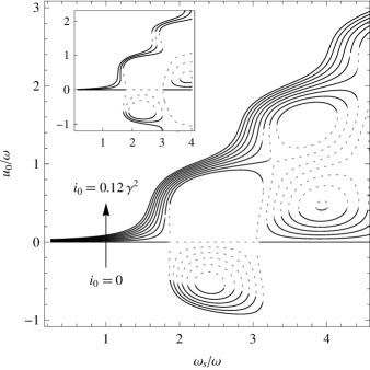
Figure 3: Generated dc voltage as a function of the drive amplitude at different bias currents. Solid curves indicate stable values while dashed curves operating points with ndc. Inset axis are the same as in main figure. Main figure: Parameters correspond to existing highly doped, wide miniband ssls: $\omega\tau=2.0$, $r\tau=2.25$, $\gamma_{\mathrm{v}}\tau=2.0$, $\gamma_{\mathrm{w}}\tau=0.5$, $\alpha\tau=0.015$, and $w_{\mathrm{eq}}=-0.75$. A range of bias currents is from $i_{0}=0$ to $i_{0}=0.12\gamma^{2}$. Inset: Parameters are pushed to higher but reasonable values, $\omega\tau=3.0$, $r\tau=5.0$, $\gamma_{\mathrm{v}}\tau=2.0$, $\gamma_{\mathrm{w}}\tau=0.5$, $\alpha\tau=0.005$, and $w_{\mathrm{eq}}=-0.75$. Bias currents range from $i_{0}=0$ to $0.39\gamma^{2}$.

We will start by considering a highly doped, wide miniband superlattice that is currently realizable. In figure 3 sample runs are presented where nearly quantized dc voltage can be achieved for parameters corresponding to such an ssl device. In the main figure, the values were chosen as $r\tau=2.25$, $\omega\tau=2.0$, $\gamma_{\mathrm{v}}\tau=2.0$, $\gamma_{\mathrm{w}}\tau=0.5$, $\alpha\tau=0.015$, and $w_{\mathrm{eq}}=-0.75$. A range of dc currents $i_{0}$ from $0$ to $0.12\gamma^{2}$ was used to demonstrate the effect of current biasing. The $i_{0}=0$ curve shows again a region of spontaneous dc near $\omega_{\mathrm{s}}/\omega\simeq 2.4$. This is surrounded as expected by ndc and here further by multistability and so stable operation is not available. As in the $\omega_{\mathrm{pl}}\tau\lesssim 1$ case, the inclusion of the dc bias removes the ndc and the multistability. For small but non-zero $i_{0}$ the ndc is not completely gone, but does disappear quickly as the bias is increased. A rapid rise in $u_{0}$ is observed near the symmetry breaking bifurcation of the $i_{0}=0$ curve ($\omega_{\mathrm{s}}/\omega\simeq 1.8$), and further, this sudden increase quickly shoulders off to form a slightly tilted plateau where $u_{0}\simeq\omega$. The realized $u_{0}$ depends only weakly on $i_{0}$, showing that the device is not sensitive to the choice of bias current as long as it is sufficiently high to remove the instabilities. Higher near-quantized plateaus for which $u_{0}/\omega\simeq n$ with $n>1$ also become available, though now the quantization is less good.

The inset in figure 3 shows what can be achieved with a reasonable push in the parameters. Here, we have boosted the plasma frequency to $r\tau=5$ and drive frequency to $\omega\tau=3.0$ while reducing the inverse parallel resistance $\alpha$ to $0.005\gamma$. Dependence on the bias current is again similar (here, $i_{0}=0\ldots 0.39\gamma^{2}$) with the case of zero external current showing instabilities that are removed as $i_{0}$ is increased. With these parameters the shoulder where $u_{0}$ levels off to $\simeq\omega$ is sharper and the quantization better, yet $u_{0}$ is single valued in $\omega_{\mathrm{s}}$ as desired. Quantization with $\eta\approx 0.95$ ($u_{0}=\eta\omega$) can be observed here for a wide range of $\omega_{\mathrm{s}}$.

Note that the $\omega_{\mathrm{pl}}\tau\lesssim 1$ limit suggests a scaling law. The equations that determine $u_{0}$, (9) and (11), depend on $r$, $\alpha$, and $i_{0}$ only via the fractions $\alpha/r^{2}$ and $i_{0}/r^{2}$. Therefore, one could hypothesize that the increased stability of $\omega_{\mathrm{pl}}\tau\gtrsim 1$ case is only due to a decrease in the effective inverse parallel resistance $\alpha/r^{2}$, and could then be replicated by keeping $r$ fixed and decreasing $\alpha$ instead. We tested this hypothesis by running simulations with fixed $\alpha/r^{2}$ and varying $r$ and found it to be false, so that increasing $r$ really does have an effect of suppressing ndc.

We see that stable operation at higher applied field frequencies can be obtained in the limit of a high plasma frequency, or a high doping and a wide miniband. Because higher $\omega\tau$ can be reached, also the quantization of the spontaneous dc voltage is improved. Nonetheless, ndc and hysteretic response still set strict limits to frequency and hence to the quantization that can be achieved. Stability against domains must be balanced against how small $|u_{0}-n\omega|$ is desired. To elaborate further on the parameters that affect the spontaneous dc, we note that there is some sensitivity to the value $\alpha$. Zero inverse parallel resistance, $\alpha=0$, results in a more hysteretic response, and so a small degree of damping in the equation for $u$ is preferable. However, for $\alpha\tau\gtrsim 0.1$ the generated dc voltage becomes close to zero, so smallness of $\alpha$ is still required. In terms of the dc bias current, the device does not appear to be very sensitive to its value as long as it is sufficient to remove ndc near zero dc voltages. Increasing $i_{0}$ further to moderate values has little effect on stability, it only shifts the point where strong response occurs to lower values of $\omega_{\mathrm{s}}/\omega$. Again, we note that since the spontaneous dc states are often stable when $i_{0}=0$, the bias current is not necessary anymore once a stable equilibrium is reached provided of course that the unbiased operating point is not in ndc.

5 Conclusions

We have presented a turn-on scheme for a semiconductor superlattice THz-rectifier that addresses the problem of stability against formation of electric domains due to ndc. While a spontaneous dc voltage state of a pure ac driven semiconductor superlattice is stable, this voltage state can only be reached by driving the device into conditions where domains do form. Our proposed solution to this problem is to apply a weak dc current bias while the applied field is adiabatically increased to its target value. The external dc bias has the effect of shifting the operating point towards higher dc voltages whereby the device shows positive differential conductivity, and therefore is stable against formation of domains. This shifting appears as a strong response in the dc voltage as a function of the amplitude of the external ac field and is seen for parameters that correspond to dynamical symmetry breaking in the pure ac driven case.

For typical superlattices and experimentally realizable parameters of applied field, together with small dc bias currents, the strong response in the dc voltage and stable switching to a spontaneous dc field state are indeed found. Appearance of ndc and hysteretic response however do still set an upper limit to the applied radiation (angular) frequencies $\omega$ that give the desired behaviour. For weak nonlinearity, $\omega$ is roughly limited by $1.5\sim 2$ times the characteristic scattering rates. Somewhat counter-intuitively, in the limit of strong nonlinearity (high plasma frequencies) stable operation can be achieved for higher drive frequencies. In accordance with previous results on generation of spontaneous dc voltage, we found the generated dc field becomes closer to an integer multiple of $\hbar\omega/ea$ as $\omega$ is increased. Therefore, our results show that for optimal, stable frequency to voltage conversion, high plasma frequencies are preferable. Our numerical results show that good quantization of the generated voltage can be achieved for realistic semiconductor superlattices. These findings demonstrate that it may indeed be possible to apply semiconductor superlattices as room temperature frequency-to-voltage converters and detectors of a strong THz radiation.

References

References

- [1] Esaki L and Tsu R 1970 IBM J. Res. Dev. 14 61
- [2] Bloch F 1928 Z. Phys. 52 555
- [3] Wacker A 2002 Phys. Rep. 357 1
- [4] Hyart T, Alekseev K N and Thuneberg E V 2008 Phys. Rev. B 77 165330
- [5] Hyart T, Alexeeva N V, Mattas J and Alekseev K N 2009 Phys. Rev. Lett. 102 140405
- [6] Hyart T, Mattas J and Alekseev K N 2009 Phys. Rev. Lett. 103 117401
- [7] Savvidis P G, Kolasa B, Lee G and Allen S J 2004 Phys. Rev. Lett. 92 196802
- [8] Sekine N and Hirakawa K 2005 Phys. Rev. Lett. 94 057408
- [9] Unuma T, Ino Y, Kuwata-Gonokami M, Bastard G and Hirakawa K 2010 Phys. Rev. B 81 125329
- [10] Tucker J R and Feldman M J 1985 Rev. Mod. Phys. 57 1055
- [11] Ignatov Anatoly A and Jauho A-P 1999 J. Appl. Phys. 85 3643
- [12] Ignatov A A, Klappenberger F, Schomburg E and Renk K F 2002 J. Appl. Phys. 91 1281
- [13] Winnerl S et al. 1997 Phys. Rev. B 56 10303
- [14] Schomburg E et al. 2000 Physica E 7 814
- [15] Klappenberger F, Ignatov A A, Winnerl S, Schomburg E, Wegscheider W, Renk K F and Bichler M 2001 Appl. Phys. Lett. 78 1674
- [16] Winnerl S et al. 1998 Appl. Phys. Lett. 73 2983
- [17] Winnerl S et al. 1999 Superlatt. Microstruct. 25 57
- [18] Alekseev K N, Berman G P, Campbell D K, Cannon E H and Cargo M C 1996 Phys. Rev. B 54 10625
- [19] Alekseev K N and Kusmartsev F V 2002 Phys. Lett. A 305 281
- [20] Dunlap D H, Kovanis V, Duncan R V and Simmons J 1993 Phys. Rev. B 48 7975
- [21] Ignatov A A, Schomburg E, Grenzer J, Renk K F and Dodin E P 1995 Z. Phys. B 98 187
- [22] Alekseev K N, Cannon E H, McKinney J C, Kusmartsev F V and Campbell D K 1998 Phys. Rev. Lett. 80 2669
- [23] Romanov Yu A and Romanova Yu Yu 2000 J. Exp. Theor. Phys. 91 1033
- [24] Romanov Yu A, Romanova J Yu, Mourokh L G and Horing N J M 2001 J. Appl. Phys. 89 3835
- [25] Alekseev K N, Cannon E H, Kusmartsev F V and Campbell D K 2001 Europhys. Lett. 56 842
- [26] Langenberg D N, Scalapino D J, Taylor B N and Eck R E 1966 Phys. Lett. 20 563
- [27] Levinsen M T, Chiao R Y, Feldman M J and Tucker B A 1977 Appl. Phys. Lett. 31 776
- [28] Ignatov A A, Renk K F and Dodin E P 1993 Phys. Rev. Lett. 70 1996
- [29] Isohätälä J and Alekseev K N 2010 Chaos 20 023116
- [30] Alekseev K N, Pietiläinen P, Isohätälä J, Zharov A A and Kusmartsev F V 2005 Europhys. Lett. 70 292
- [31] Bumyalene S, Lasene G and Piragas K 1989 Fiz. Tekh. Poluprovodn. (S.-Petersburg) 23 1479
- [32] Bumyalene S, Lasene G and Piragas K 1989 Sov. Phys. Semicond. 23 918 (Engl. Transl.)
- [33] Pavlovich V V and Epshtein E M 1976 Fiz. Tekh. Poluprovodn. (S.-Petersburg) 10 2001
- [34] Pavlovich V V and Epshtein E M 1976 Sov. Phys. Semicond. 10 1196 (Engl. Transl.)
- [35] Ignatov A A and Romanov Yu A 1976 Phys. Stat. Sol. B 73 327
- [36] Keay B J, Zeuner S, Allen S J, Maranowski K D, Gossard A C, Bhattacharya U and Rodwell M J W 1995 Phys. Rev. Lett. 75 4102
- [37] Romanov Yu A, Romanova J Yu and Mourokh L G 2009 Phys. Rev. B 79 245320
- [38] Romanov Yu A, Romanova J Yu, Mourokh L G and Horing N J M 2004 Semicond. Sci. Technol. 19 S80
- [39] Romanov Yu A, Romanova J Yu and Mourokh L G 2006 J. Appl. Phys. 99 013707
- [40] Alekseev K N, Gorkunov M V, Demarina N V, Hyart T, Alexeeva N V and Shorokhov A V 2006 Europhys. Lett. 73 934
- [41] Ghosh A W, Wanke M C, Allen S J and Wilkins J W 1999 Appl. Phys. Lett. 74 2164
- [42] Schomburg E, Henini M, Chamberlain J M, Steenson D P, Brandl S, Hofbeck K, Renk K F and Wegscheider W 1999 Appl. Phys. Lett. 74 2179
- [43] Isohätälä J, Alekseev K N, Kurki L T and Pietiläinen P 2005 Phys. Rev. E 71 066206
- [44] Ridley B K and Watkins T B 1961 Proc. Phys. Soc. 78 293
- [45] Ktitorov S A, Simin G S and Sindalovskii V Ya 1971 Fiz. Tverd. Tela 13 2230
- [46] Ktitorov S A, Simin G S and Sindalovskii V Ya 1972 Sov. Phys. Solid State 13 1872 (Engl. Transl.)
- [47] Büttiker M and Thomas H 1977 Phys. Rev. Lett. 38 78
- [48] Klappenberger F et al. 2004 Eur. Phys. J. B 39 483
- [49] Bass F G and Bulgakov A A 1997 Kinetic and Electrodynamic Phenomena in Classical and Quantum Semiconductor Superlattices (New York: Nova)
- [50] Platero G and Aguado R 2004 Phys. Rep. 395 1
- [51] Tien P K and Gordon J P 1963 Phys. Rev. 129 647