Effective dipole-dipole interactions in multilayered dipolar Bose-Einstein condensates

Abstract

We propose a two-dimensional model for a multilayer stack of dipolar Bose-Einstein condensates formed by a strong optical lattice. We derive effective intra- and interlayer dipole-dipole interaction potentials and provide simple analytical approximations for a given number of lattice sites at arbitrary polarization. We find that the interlayer dipole-dipole interaction changes the transverse aspect ratio of the ground state in the central layers depending on its polarization and the number of lattice sites. The changing aspect ratio should be observable in time of flight images. Furthermore, we show that the interlayer dipole-dipole interaction reduces the excitation energy of local perturbations affecting the development of a roton minimum.

I Introduction

Layered structures of magnetic materials play a crucial role both in today’s technology and in fundamental physical theories. Technological examples are aplenty in the magneto-electronic industries, e.g., hard disks or magnetic sensors. One theoretical goal of studying multilayers is to illuminate the elusive theory of high-$T_{c}$ superconductivity, where the layered structure appears to play a crucial role Lee et al. (2006). For a realistic theory of atomic or molecular multilayers it is, however, vital to include the dipole-dipole interaction (DDI) between the underlying particles.

The study of magnetic single- and multilayer films has enjoyed a long history in condensed matter physics (for a recent review, see Ref. De’Bell et al. (2000) and references therein). There, an alternating structure of ferromagnetic and nonmagnetic layers is deposited on a substrate, e.g., by atomic beam epitaxy. However, structural instabilities induced, e.g., by temperature changes and film thickness variation often complicate experiments in thin films.

Quantum-degenerate dipolar gases have received much attention recently from both theoretical and experimental studies (for recent reviews, see Refs. Lahaye et al. (2009); Baranov (2008)). Their DDI crucially affects the ground-state properties Góral et al. (2000); Yi and You (2000), stability Santos et al. (2000, 2003); Fischer (2006), and dynamics of the gas Yi and You (2001). Furthermore, they offer a route for studying exciting many-body quantum effects, such as a superfluid-to-crystal quantum phase transition Büchler et al. (2007), supersolids Góral et al. (2002) or even topological order Micheli et al. (2006). Recent advances in experimental techniques have paved the way for a Bose-Einstein condensate (BEC) of ⁵²Cr with a magnetic dipole moment $6\mu_{B}$ (Bohr magneton $\mu_{B}$), much larger than conventional alkali BECs Griesmaier et al. (2005); Stuhler et al. (2005); Koch et al. (2008). Promising candidates for future dipolar BEC experiments are Er and Dy with even larger magnetic moments of $7\mu_{B}$ and $10\mu_{B}$, respectively Berglund et al. (2008); Lu et al. (2010). Furthermore, DDI-induced decoherence and spin textures have been observed in alkali-metal condensates Fattori et al. (2008); Vengalattore et al. (2008). Dipolar effects also play a crucial role in experiments with Rydberg atoms Vogt et al. (2006) and heteronuclear molecules Ni et al. (2010); de Miranda et al. (2011). Bosonic heteronuclear molecules may provide a basis for future experiments on BECs with dipole moments much larger than in atomic BECs Voigt et al. (2009).

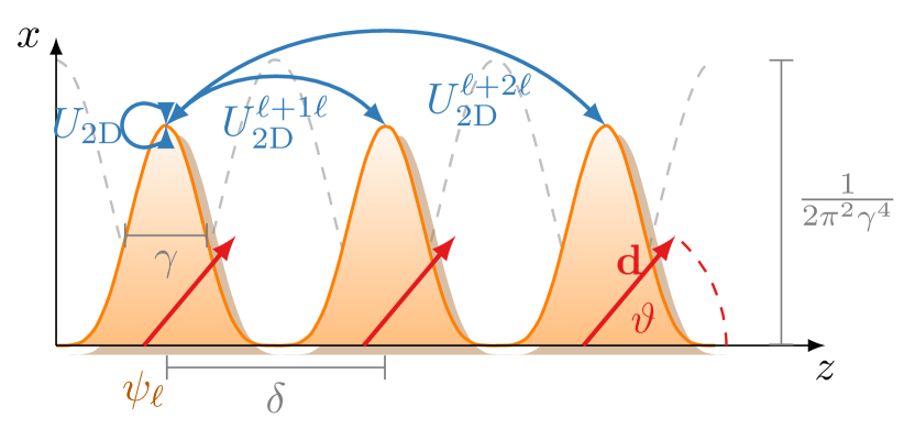
Figure 1: (Color online) Setup of the multilayered dipolar BEC polarized along $\boldsymbol{\mathrm{d}}$. An optical lattice along $z$ separates the dipolar BEC into 2D layers in the $x$–$y$ plane with distance $\delta$. Apart from the intralayer DDI $U_{\text{2D}}$, each layer interacts with other layers via the interlayer DDI $U_{\text{2D}}^{j\ell}$.

In contrast to solid state thin film structures, the layer width and spacing of BECs in optical lattices are precisely tunable with external fields. This makes dipolar BECs a prime candidate for investigating the effects of DDI in multilayers. For example, it has been shown that the DDI stabilizes quasi-two-dimensional ultracold gases for perpendicular polarization Fischer (2006); Müller et al. (2011) and enables controlled chemical reactions de Miranda et al. (2011). Another intriguing effect is the occurrence of interlayer bound states Klawunn et al. (2010); Baranov et al. (2011); Shih and Wang (2009); Potter et al. (2010); Rosenkranz and Bao (2011); Volosniev et al. (2011a). However, it is still unclear to what extend effective models for multilayers of dipolar BEC at arbitrary polarization are valid and how interlayer DDI can be detected.

In this article, we investigate the effect of interlayer DDI on the ground state of the BEC. We present an effective two-dimensional (2D) model for an arbitrarily polarized dipolar BEC in a strong one-dimensional (1D) optical lattice. Our 2D model offers a clear advantage for numerical computation of ground state properties compared to computations for a full three-dimensional (3D) Gross-Pitaevskii equation (GPE): our computation times reduce to seconds instead of dozens of hours. Previously, such dimension-reduced models have been derived for BECs without DDI Bao and Tang (2003); Bao et al. (2003); Salasnich (2009); Abdallah et al. (2005, 2008); Lieb et al. (2003); Yngvason et al. (2004) and with dipolar interactions in a single layer Carles et al. (2008); Cai et al. (2010). We also derive the effective 2D intra- and interlayer DDI potentials governing the layers of quasi-2D BECs. These potentials allow for useful analytical approximations, which were used in a previous work on multilayer dipolar BECs with perpendicular polarization Baranov et al. (2011). We establish that the 2D model is valid by comparing its ground states to ground states of the 3D GPE for weakly interacting BECs at zero temperature Pitaevskii and Stringari (2003). We suggest that the interlayer DDI is observable in the transverse aspect ratio of the central layers after time of flight expansion. Moreover, we calculate the Bogoliubov excitation energies for a transversely homogeneous BEC with contact, intra- and interlayer DDI. The interlayer DDI reduces the squared Bogoliubov energy and, therefore, influences the occurance of a roton minimum.

In Sec. II we present our 2D model and effective intra- and interlayer potentials for a dipolar BEC trapped in a strong 1D optical lattice. We also present a single mode approximation valid for the central layers of the BEC. In Sec. III we compare ground states of our model and its single mode approximation to ground states of the 3D GPE. We find good agreement between these ground states, which indicates the validity of our model. In Sec. IV we compute numerically the aspect ratio of the BEC in the central layer as a function of the number of lattice sites and polarization direction. We find a marked change in the aspect ratio owing to the interlayer DDI, which should be observable in experiments. In Sec. V we derive the Bogoliubov dispersion for a transverse homogeneous, multilayered dipolar BEC. We conclude in Sec. VI. In App. A we give a detailed derivation of the 2D model presented in Sec. II.

II Effective 2D model

We consider a dilute dipolar BEC at zero temperature trapped in a transverse harmonic potential $V_{\text{ho}}(x,y)=\tfrac{m\omega^{2}}{2}(x^{2}+y^{2})$ and a longitudinal optical lattice $V_{\text{o}}(z)=V_{0}\sin^{2}(k_{l}z)$. Here, $m$ is the particle mass, $\omega$ the trap frequency, $V_{0}$ the lattice height, and $k_{l}$ the wave number of the lattice laser. We focus on atomic BECs with a magnetic dipole moment but it is straightforward to extend the analysis to degenerate bosonic gases with electric dipole moments. We assume that an external field polarizes the atoms along a normalized axis $\boldsymbol{\mathrm{d}}=(d_{x},d_{y},d_{z})=(\cos\phi\sin\vartheta,\sin\phi\sin\vartheta,\cos\vartheta)$ with $\phi$ and $\vartheta$ the azimuthal and polar angles, respectively. Then the dipole-dipole interaction (DDI) is described by

$$U_{\text{dd}}(\boldsymbol{\mathrm{r}})=\frac{c_{\text{dd}}}{4\pi}\frac{|\boldsymbol{\mathrm{r}}|^{2}-3(\boldsymbol{\mathrm{d}}\cdot\boldsymbol{\mathrm{r}})^{2}}{|\boldsymbol{\mathrm{r}}|^{5}},$$ (1)

where $c_{\text{dd}}=\mu_{0}D^{2}$ with $\mu_{0}$ is the magnetic vacuum permeability and $D$ the dipole moment (for electric dipoles $c_{dd}=D^{2}/\epsilon_{0}$, where $\epsilon_{0}$ is the vacuum permittivity). We note that it is possible to modify the DDI strength $c_{\text{dd}}$ by means of a rotating magnetic field Giovanazzi et al. (2002).

At zero temperature, a weakly interacting BEC is described by the GPE Pitaevskii and Stringari (2003). For simplicity, we introduce dimensionless quantities by rescaling lengths with the lattice distance $\delta=\pi/k_{l}$, that is, $\boldsymbol{\mathrm{r}}\rightarrow\boldsymbol{\mathrm{r}}\delta$, energies with $\hbar^{2}/m\delta^{2}=2E_{r}/\pi^{2}$ ($E_{r}$ is the recoil energy), and the wave function of the gas with the central density $n(0)$, $\psi\rightarrow\psi\sqrt{n(0)}$. In these units the normalization of the wave function is $\int d^{3}\boldsymbol{\mathrm{r}}|\psi(\boldsymbol{\mathrm{r}},t)|^{2}=N/n(0)\delta^{3}$ with $N$ the total number of atoms. Away from shape resonances, the wave function $\psi=\psi(\boldsymbol{\mathrm{r}},t)$ of the dipolar BEC is governed by the GPE Marinescu and You (1998); Yi and You (2000); Deb and You (2001)

$$i\partial_{t}\psi=\left[-\frac{1}{2}\nabla^{2}+V_{\text{ho}}+V_{\text{o}}+(g-g_{d})|\psi|^{2}+V_{\text{dd}}\right]\psi.$$ (2)

Here, $g=4\pi a_{s}n(0)\delta^{2}$ is the dimensionless contact interaction strength with $a_{s}$ the s-wave scattering length and $g_{d}=mc_{\text{dd}}n(0)\delta^{2}/3\hbar^{2}$ is the dimensionless DDI strength. Furthermore, $V_{\text{ho}}(\boldsymbol{\mathrm{\rho}})=(m^{2}\omega^{2}\delta^{4}/2\hbar^{2})\boldsymbol{\mathrm{\rho}}^{2}$ with $\boldsymbol{\mathrm{\rho}}=(x,y)$ and $V_{\text{o}}(z)=(\bar{V}_{0}\pi^{2}/2)\sin^{2}(\pi z)$, where $\bar{V}_{0}$ is the lattice amplitude in units of the recoil energy $E_{r}$. The nonlocal dipolar potential $V_{\text{dd}}$ is given by

$$V_{\text{dd}}(\boldsymbol{\mathrm{r}})=-3g_{d}\partial_{\boldsymbol{\mathrm{d}}\boldsymbol{\mathrm{d}}}\int d^{3}\boldsymbol{\mathrm{r}}^{\prime}U_{\text{3D}}(\boldsymbol{\mathrm{r}}-\boldsymbol{\mathrm{r}}^{\prime})|\psi(\boldsymbol{\mathrm{r}}^{\prime},t)|^{2}$$ (3)

with the kernel $U_{\text{3D}}(\boldsymbol{\mathrm{r}})=1/4\pi|\boldsymbol{\mathrm{r}}|$ and the notation $\partial_{\boldsymbol{\mathrm{d}}}=\boldsymbol{\mathrm{d}}\cdot\boldsymbol{\mathrm{\nabla}}$, $\partial_{\boldsymbol{\mathrm{d}}\boldsymbol{\mathrm{d}}}=\partial_{\boldsymbol{\mathrm{d}}}^{2}$.

II.1 Coupled modes

For strong optical lattices we derive an effective 2D equation for the wave function on each lattice site. This is possible because a strong optical lattice with $V_{0}\gg\hbar\omega$ causes the BEC to form layers separated by the lattice distance $\delta$ (cf. Fig. 1) Burger et al. (2002); Pitaevskii and Stringari (2003). We assume that the axial extend $\gamma$ of the BEC in each layer is much larger than the s-wave scattering length. Additionally, in the quasi-2D regime $\gamma^{-2}\gg|g-g_{d}|$ Petrov et al. (2000). This condition allows us to approximate the optical lattice as a train of harmonic potentials and the axial wave function as its ground state. Then the wave function separates into $\psi(\boldsymbol{\mathrm{r}},t)=\mathrm{e}^{-\mathrm{i}t/2\gamma^{2}}\sum_{\ell}\psi_{\ell}(\boldsymbol{\mathrm{\rho}},t)w_{\ell}(z)$ Bao et al. (2003); Pitaevskii and Stringari (2003); Cai et al. (2010). The sum extends over all lattice sites $\ell$. Under our assumptions the axial wave function on each site $\ell$ at position $z_{\ell}$ is described by a Gaussian $w_{\ell}(z)=w(z-z_{\ell})=(1/\pi\gamma^{2})^{1/4}\mathrm{e}^{-(z-z_{\ell})^{2}/2\gamma^{2}}$; the Gaussians do not mutually overlap ($\int dzw_{\ell}(z)w_{j}(z)\simeq 0$ for $\ell\neq j$). In the quasi-2D limit $\gamma^{-2}=\sqrt{\bar{V}_{0}}\pi^{2}$. More generally, in a homogeneous BEC it is also possible to treat the layer width $\gamma$ as a variational parameter that minimizes the Gross-Pitaevskii energy functional Fischer (2006). By inserting this wave function into Eq. (2) and integrating out the $z$ direction we obtain the following equation for the radial wave function $\psi_{\ell}=\psi_{\ell}(\boldsymbol{\mathrm{\rho}},t)$ at site $\ell$

$$\mathrm{i}\partial_{t}\psi_{\ell}=\left[-\frac{1}{2}\nabla^{2}+V_{\text{ho}}+\bigl{[}\bar{g}-\bar{g}_{d}\bigl{(}1-3d_{z}^{2}\bigr{)}\bigr{]}|\psi_{\ell}|^{2}+V_{\text{2D}}^{\ell}\right]\psi_{\ell}.$$ (4)

Here, $\bar{g}=g/\sqrt{2\pi}\gamma$ and $\bar{g}_{d}=g_{d}/\sqrt{2\pi}\gamma$ are the effective 2D interactions strengths. In the remainder of this article we neglect strongly suppressed terms in the effective DDI potential $V_{\text{2D}}^{\ell}$ (see Appendix A for details). We find the following expression for its Fourier transform $\hat{V}_{\text{2D}}^{\ell}(\boldsymbol{\mathrm{k}})=\mathcal{F}[V_{\text{2D}}^{\ell}](\boldsymbol{\mathrm{k}})$ with $\boldsymbol{\mathrm{k}}=k(\cos\varphi,\sin\varphi)$

$$\begin{split}\hat{V}_{\text{2D}}^{\ell}(\boldsymbol{\mathrm{k}})&=3g_{d}\sum_{j}\Bigl{(}\left[(d_{x}\cos\varphi+d_{y}\sin\varphi)^{2}-d_{z}^{2}\right]\hat{U}_{\text{even}}^{j\ell}(k)\\ &\quad+2\mathrm{i}d_{z}(d_{x}\cos\varphi+d_{y}\sin\varphi)\hat{U}_{\text{odd}}^{j\ell}(k)\Bigr{)}\widehat{|\psi_{j}|^{2}}(\boldsymbol{\mathrm{k}}).\end{split}$$ (5)

Here,

$$\hat{U}_{\text{even}}^{j\ell}(k) =\frac{k}{4}\mathrm{e}^{-\tfrac{\delta_{\ell j}^{2}}{2\gamma^{2}}}\left[\eta\left(\frac{\gamma^{2}k+\delta_{\ell j}}{\sqrt{2}\gamma}\right)+\eta\left(\frac{\gamma^{2}k-\delta_{\ell j}}{\sqrt{2}\gamma}\right)\right],$$ (6)

$$\hat{U}_{\text{odd}}^{j\ell}(k) =\frac{k}{4}\mathrm{e}^{-\tfrac{\delta_{\ell j}^{2}}{2\gamma^{2}}}\left[\eta\left(\frac{\gamma^{2}k+\delta_{\ell j}}{\sqrt{2}\gamma}\right)-\eta\left(\frac{\gamma^{2}k-\delta_{\ell j}}{\sqrt{2}\gamma}\right)\right],$$ (7)

where $\delta_{\ell j}=(\ell-j)$, $\eta(x)=\exp(x^{2})\operatorname{erfc}(x)$ and $\operatorname{erfc}(x)=1-\operatorname{erf}(x)$ is the complementary error function.

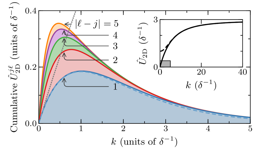
Figure 2: (Color online) Cumulative interlayer DDI $\hat{U}_{\text{2D}}^{j\ell}$ for ⁵²Cr at different layer separations $|\ell-j|$. The solid lines show the interlayer DDI [Eq. (9)], whereas the dashed line shows the approximation Eq. (10) for nearest neighbors [Eq. (10) is indistinguishable from the solid lines for larger distances]. The dotted line indicates the intralayer DDI. The inset shows the intralayer DDI and the rectangle within indicates the extend of the main panel. We set $V_{0}=30E_{r}$.

The effective dipolar interaction $\hat{V}_{\text{2D}}^{\ell}$ [Eq. (5)] contains both an intralayer DDI and an interlayer DDI. The intralayer DDI are the terms in Eq. (5) with $\ell=j$. By setting $\ell=j$ in Eqs. (6)-(7) we find that each layer experiences the effective DDI potential of a quasi-2D dipolar BEC Cai et al. (2010). The interlayer DDI are the terms in Eq. (5) with $\ell\neq j$. For perpendicular polarization ($d_{z}=1$, $d_{x}=d_{y}=0$) we recover the interlayer DDI potential discussed, e.g., in Ref. Baranov et al. (2011). If the layer distance is much larger than the layer width ($|\delta_{\ell j}|\gg\gamma$), $\eta(x\rightarrow+\infty)$ vanishes and the moduli of the kernels $|\hat{U}_{\text{even}}^{j\ell}|$ and $|\hat{U}_{\text{odd}}^{j\ell}|$ become identical. Because of our assumption that $\delta\gg\gamma$, this is fulfilled for the interlayer DDI between any two distinct sites. As a consequence, we split the total effective DDI potential into a sum of intralayer and interlayer terms

$$\begin{split}\hat{V}_{\text{2D}}^{\ell}(\boldsymbol{\mathrm{k}})&=3g_{d}[(d_{x}\cos\varphi+d_{y}\sin\varphi)^{2}-d_{z}^{2}]\hat{U}_{\text{2D}}(k)\widehat{|\psi_{\ell}|^{2}}(\boldsymbol{\mathrm{k}})\\ &\quad+3g_{d}\sum_{j\neq\ell}[d_{x}\cos\varphi+d_{y}\sin\varphi-\mathrm{i}d_{z}\operatorname{sgn}(\delta_{\ell j})]^{2}\\ &\quad\times\hat{U}_{\text{2D}}^{j\ell}(k)\widehat{|\psi_{j}|^{2}}(\boldsymbol{\mathrm{k}}),\end{split}$$ (8)

where $\operatorname{sgn}(x)$ is the sign of $x$. The kernels of this potential are $\hat{U}_{\text{2D}}=2\hat{U}_{\text{2D}}^{00}$ and

$$\hat{U}_{\text{2D}}^{j\ell}(k)=\frac{k}{4}\mathrm{e}^{-\frac{\delta_{\ell j}^{2}}{2\gamma^{2}}}\eta\left(\frac{\gamma^{2}k-|\delta_{\ell j}|}{\sqrt{2}\gamma}\right).$$ (9)

In the limit of negligible layer width ($\gamma\ll|\delta_{\ell j}|$) the interlayer DDI in Eq. (9) can be approximated by

$$\hat{U}_{\text{2D}}^{j\ell}(k)\simeq\frac{k}{2}\mathrm{e}^{-|\delta_{\ell j}|k}\quad(\ell\neq j).$$ (10)

This approximation becomes an identity in the limit $\gamma\rightarrow 0$ and nonzero $|\delta_{\ell j}|$. The second line of Eq. (8) is the interlayer DDI potential for arbitrary polarization direction. Inserting approximation (10) into Eq. (8) for perpendicular polarization, we recover the interlayer DDI potential used in Refs. Potter et al. (2010); Baranov et al. (2011). We expect our generalized interlayer DDI potential to be valid for bosons as well as fermions because fermions in different layers occupy different quantum states.

The kernel of the interlayer DDI potential $\hat{U}_{\text{2D}}^{j\ell}(k)$ is shown in Fig. 2 as a cumulative plot over the five nearest lattice sites. For comparison we also show the intralayer DDI. Although not shown in Fig. 2, we established that for realistic parameters the potentials $\hat{U}_{\text{even}}^{j\ell}$ and $\hat{U}_{\text{odd}}^{j\ell}$ (for $\ell\neq j$) are indistinguishable from $\hat{U}_{\text{2D}}^{j\ell}$ at the plot resolution. For interlayer interactions beyond nearest neighbors the approximation for $\hat{U}_{\text{2D}}^{j\ell}$ in Eq. (10) becomes indistinguishable from Eq. (9). The interlayer DDI is linear in momentum for long wavelengths and drops exponentially for short wavelengths. It has been shown that this behavior leads to very weakly bound states in bilayer systems Volosniev et al. (2011a, b); Baranov et al. (2011); Rosenkranz and Bao (2011). According to Eq. (8) its sign is determined by the polarization direction. The interlayer and intralayer DDI for predominantly perpendicular polarization ($\vartheta<\pi/4$) is attractive in momentum space for all $\boldsymbol{\mathrm{k}}$, whereas the interlayer DDI for predominantly parallel polarization ($\vartheta>\pi/4$) becomes repulsive for some $\boldsymbol{\mathrm{k}}$ around the major axis with $\varphi=\phi$.

II.2 Single mode approximation

If we assume that the the BEC densities in each layer vary little over the central sites, we can simplify the 2D model to a single equation for the central site wave function $\psi_{0}(\boldsymbol{\mathrm{\rho}})$. This assumption is reasonable for large lattices and we will test its validity in Sec. III. The single wave function $\psi_{0}(\boldsymbol{\mathrm{\rho}})$ approximates the wave functions in all lattice sites far from the boundaries. Consequently, we replace the effective dipolar potential $\hat{V}_{\text{2D}}^{\ell}(\boldsymbol{\mathrm{k}})$ [Eq. (8)] by the site-local potential

$$\begin{split}\hat{V}_{\text{2D}}(\boldsymbol{\mathrm{k}})&=3g_{d}\Bigl{(}[(d_{x}\cos\varphi+d_{y}\sin\varphi)^{2}-d_{z}^{2}]\hat{U}_{\text{2D}}(k)\\ &\quad+\sum_{j\neq 0}[d_{x}\cos\varphi+d_{y}\sin\varphi-\mathrm{i}d_{z}\operatorname{sgn}(j)]^{2}\hat{U}_{\text{2D}}^{j0}(k)\Bigr{)}\\ &\quad\times\widehat{|\psi_{0}|^{2}}(\boldsymbol{\mathrm{k}}).\end{split}$$ (11)

Inserting the inverse Fourier transform of Eq. (11) into Eq. (4) we are left with the uncoupled equation

$$\mathrm{i}\partial_{t}\psi_{0}=\left[-\frac{1}{2}\nabla^{2}+V_{\text{ho}}+\bigl{[}\bar{g}-\bar{g}_{d}\bigl{(}1-3d_{z}^{2}\bigr{)}\bigr{]}|\psi_{0}|^{2}+V_{\text{2D}}\right]\psi_{0}$$ (12)

for the central site wave function $\psi_{0}=\psi_{0}(\boldsymbol{\mathrm{\rho}})$. We assume a lattice that is symmetric around the central site so that the dipole terms linear in $d_{z}$ in Eq. (11) vanish after summation. Using Eq. (10) for $\hat{U}_{\text{2D}}^{j0}$ we can perform the summation in Eq. (11) and find

$$\begin{split}\hat{V}_{\text{2D}}(\boldsymbol{\mathrm{k}})&\simeq 3g_{d}[(d_{x}\cos\varphi+d_{y}\sin\varphi)^{2}-d_{z}^{2}]\\ &\quad\times\bigl{[}\hat{U}_{\text{2D}}(k)+\hat{U}_{\text{2D}}^{N_{s}^{*}}(k)\bigr{]}\widehat{|\psi_{0}|^{2}}(\boldsymbol{\mathrm{k}})\end{split}$$ (13)

with

$$\hat{U}_{\text{2D}}^{N_{s}^{*}}(k)=k\left(\frac{1-\mathrm{e}^{-(N_{s}^{*}+1)k/2}}{1-\mathrm{e}^{-k}}-1\right).$$ (14)

Here, we summed over $N_{s}^{*}$ central lattice sites. In the limit of an infinite lattice the maximum of $U_{\text{2D}}^{N_{s}^{*}}$ moves towards $k=0$ with $\lim_{k\rightarrow 0}\hat{U}_{\text{2D}}^{\infty}(k)=1$. Therefore, the total DDI potential for an infinite stack of BECs does not vanish anymore at $k=0$ (dashed line in the inset of Fig. 2). However, this is a pathological case because for any finite $N_{s}$ the total DDI potential vanishes at $k=0$ and our assumption of slowly varying wave functions breaks down towards the boundary.

III Validity of the 2D model

In this section, we investigate the validity of the effective 2D model for multilayered dipolar BECs introduced in Sec. II. To this end we computed ground states for the 3D GPE [Eq. (2)]  Bao et al. (2010), the coupled 2D model [Eq. (4)] Bao (2004), and the single mode 2D model [Eq. (12)] Bao and Du (2004) using the normalized gradient flow (imaginary time) method. For the time discretization we used backward Euler finite difference Bao and Du (2004). For the spatial discretization we employed the sine pseudospectral Bao et al. (2010) and the Fourier pseudospectral methods Cai et al. (2010) for the 3D GPE and the 2D models, respectively. For the 3D computation we assumed that the wave function vanishes at the boundaries. We integrated the 3D ground states over the individual lattice sites to find the $N_{s}$ densities $|\psi_{\ell}^{\text{3D}}(\boldsymbol{\mathrm{\rho}})|^{2}=\int_{\delta(\ell-1/2)}^{\delta(\ell+1/2)}dz|\psi(\boldsymbol{\mathrm{r}})|^{2}$. To determine the validity of the 2D model we compared the 2D ground states $\psi_{\ell}(\boldsymbol{\mathrm{\rho}})$ to $\psi_{\ell}^{\text{3D}}(\boldsymbol{\mathrm{\rho}})$. Using the single mode approximation reduced the computation times drastically: typically to less than a minute, compared to $2$–$3$ hours for the coupled equations and $\sim 1$ day for the 3D GPE. In this section we only consider polarization in the $x$–$z$ plane, that is $\boldsymbol{\mathrm{d}}=(\sin\vartheta,0,\cos\vartheta)$ (cf. Fig. 1). Because the external potential is radially symmetric, this simplification corresponds to choosing the transverse projection of the polarization direction as the $x$ axis.

To compare the axial profiles of the coupled 2D and 3D ground states we computed the relative particle numbers in each lattice site. Because of the long range of the DDI, we observe fairly pronounced boundary effects in the 3D computations for strong dipolar interactions $g_{d}\simeq g$. For this reason we omit the $N_{b}$ outermost lattice sites in the overall normalization. Then the relative number of particles in site $\ell$ for the 2D model is given by $N_{\ell}=\int d^{2}\boldsymbol{\mathrm{\rho}}|\psi_{\ell}(\boldsymbol{\mathrm{\rho}})|^{2}/\sum_{j=-N_{s}+N_{b}}^{N_{s}-N_{b}}\int d^{2}\boldsymbol{\mathrm{\rho}}|\psi_{\ell}(\boldsymbol{\mathrm{\rho}})|^{2}$ (the relative particle number $N_{\ell}^{\text{3D}}$ for the 3D GPE follows by replacing $|\psi_{\ell}|^{2}$ with $|\psi_{\ell}^{\text{3D}}|^{2}$). Figure 3 shows the particle number difference $(N_{\ell}^{\text{3D}}-N_{\ell})/N_{0}^{\text{3D}}$ relative to the particle number at the central lattice site. Although the number difference varies slightly over the central lattice sites, the difference between the GPE and the 2D model Eq. (4) remains smaller than $4\%$ and $1\%$ for the two parameter sets, respectively.

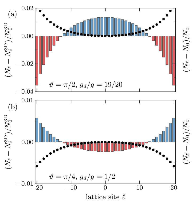
Figure 3: (Color online) Relative particle number difference between GPE ground state and the 2D model [Eq. (4)] for individual lattice sites. The particle numbers are relative to the particle number in the central layer $N_{0}^{\text{3D}}$ (bars). The discs indicate the particle number difference in the 2D model relative to the central site (right axis label). The parameters are $N_{s}=61$ lattice sites with $V_{0}=20E_{r}$, $E_{r}/\hbar\omega=60$, and $g=100\sqrt{2E_{r}/\hbar\omega\pi^{2}}$.

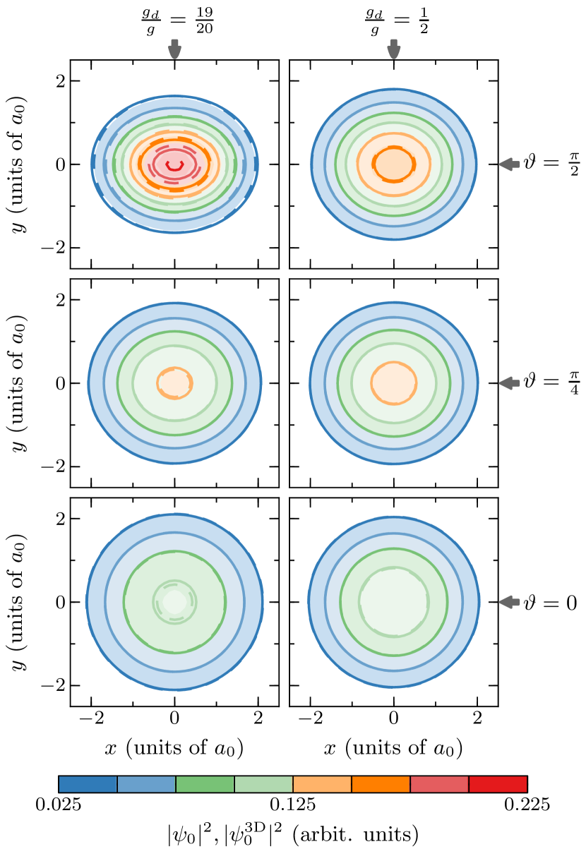
Figure 4: (Color online) Ground state densities of the central lattice site for various DDI strengths and polarization angles. The filled surfaces are the projection of the central site of the GPE results, whereas the solid (dashed) contour lines are the ground states of the coupled (single mode) 2D equation (4). The plotted densities are all normalized to $1$. The coupled and single mode results are almost indistinguishable except in the top left panel. The parameters are as in Fig. 3. The plots use the magnetic length $a_{0}=\sqrt{\hbar/m\omega}$ as length unit.

Next we compared the density profiles of the central lattice site $|\psi_{0}(\boldsymbol{\mathrm{\rho}})|^{2}$ for the coupled and single mode models with $|\psi_{0}^{\text{3D}}(\boldsymbol{\mathrm{\rho}})|^{2}$. The sum of the densities of the coupled 2D and the total density of the 3D GPE are normalized to a function proportional of the total particle number $\mathcal{N}(N)$. However, in the single mode approximation we only consider a single wave function which has, consequently, a normalization less than $\mathcal{N}$. If the BEC density were the same in all layers, the normalization of this single wave function would be $\mathcal{N}/\sqrt{N_{s}}$. Because the density varies slightly across layers, instead we chose to normalize the single mode density to the particle number in the central layer of the GPE. The ground state densities for various DDI strengths and polarization angles are shown in Fig. 4. We find that both the coupled and single mode models describe the ground state well for any polarization. We only observe a slight difference between the models for strong DDI on the order of the contact interaction and parallel polarization (top left panel in Fig. 4). This means that even the single mode approximation describes the ground state of the multilayer dipolar BEC well. Its accuracy diminishes for strong DDI because the true densities vary sufficiently strongly over the central lattice sites.

IV Interlayer-DDI-induced change of the aspect ratio

The interlayer DDI can cause observable effects in multilayered dipolar BECs. This becomes apparent from Fig. 2. The strength of the interlayer DDI is comparable to the strength of the intralayer DDI at wavelengths larger than $\delta$. We expect that the anisotropy of the DDI for $\vartheta>0$ leads to a change in the aspect ratio of a quasi-2D dipolar BEC in the central layer of a stack of dipolar BECs. In this section, we investigate these effects numerically using the single mode approximation for the central layer.

To determine the mean radii of the central layer first we computed ground state densities for a varying number of lattice sites at a constant normalization. We calculated the mean radii as

$$R_{\alpha}^{2}=\int d^{2}\boldsymbol{\mathrm{\rho}}\alpha^{2}|\psi_{0}(\boldsymbol{\mathrm{\rho}})|^{2},\quad(\alpha=x,y).$$ (15)

The aspect ratio of the central layer is then given by $R_{y}/R_{x}$. Magnetostriction causes the dipolar BEC to expand along the polarization direction Lahaye et al. (2009); Cai et al. (2010). Figure 5 shows the aspect ratio as well as the individual mean radii of the BEC as a function of the number of lattice sites $N_{s}$. The case $N_{s}=1$ corresponds to a single layer dipolar BEC. We observe that the interlayer DDI causes an additional reduction in the aspect ratio depending on the number of lattice sites and polarization angle. For perpendicular polarization the aspect ratio remains unchanged because the DDI is isotropic. However, the individual radii decrease. We have also computed aspect ratios for a stronger lattice with $V_{0}=40E_{r}$ and observed a similar dependence of the mean radii on $N_{s}$. For this stronger lattice and $\vartheta=\pi/4$ the aspect ratio was closer to $1$ and its change slightly smaller than at $V_{0}=20E_{r}$. For perpendicular polarization the mean radii and aspect ratio were nearly indistinguishable from the top panel in Fig. 5. The DDI-induced change of aspect ratio has been observed in a single layer ⁵²Cr via time of flight expansionStuhler et al. (2005); Lahaye et al. (2007). We suggest that the dependence of the aspect ratio on $N_{s}$ could also be observed via time of flight expansion. To observe the central layers, in this experiment the outer layers would have to be removed on a time scale short enough to suppress equilibration, e.g., with additional lasers focused on the outer layers. This is followed immediately by time of flight expansion of the BEC. The observable effect is largest for parallel polarization $\vartheta=\pi/2$.

Figure 5: (Color online) Mean radii and aspect ratio of the central BEC layer as a function of the number of lattice sites. The different panels correspond to different polarization angles. The interlayer DDI has a noticeable effect over several lattice sites. The lines are marked at the right and are only to guide the eye. The parameters are as in Fig. 3 with $g_{d}/g=19/20$.

V Bogoliubov excitations

In this section we investigate the influence of interlayer DDI on the excitation spectrum of a layered quasi-2D dipolar BEC. In particular, we consider local density fluctuations of the layered BEC and derive their Bogoliubov energy. Their Bogoliubov energy can assume imaginary values for suitable parameters, which indicates the onset of a dynamical instability that leads to exponential growth of excitations.

To determine the Bogoliubov energy we consider small perturbations around the ground state of Eq. (4). For simplicity we assume a vanishing transverse harmonic potential $V_{\text{ho}}=0$ and homogeneous density $\nu$ in each layer. For an optical lattice with $N_{s}$ sites $\nu=1/N_{s}$. A stationary state of the effective 2D GPE (4) is given by $\psi_{\ell}(\boldsymbol{\mathrm{\rho}},t)=\psi_{\ell}(t)=\mathrm{e}^{-\mathrm{i}\mu t}\sqrt{\nu}$ with the chemical potential

$$\mu=[\bar{g}-\bar{g}_{d}(1-3d_{z}^{2})]\nu.$$ (16)

Now we add a local perturbation $\xi_{\ell}(\boldsymbol{\mathrm{\rho}},t)$ to the stationary state $\psi_{\ell}(t)$, that is, $\psi_{\ell}(\boldsymbol{\mathrm{\rho}},t)=\mathrm{e}^{-\mathrm{i}\mu t}[\sqrt{\nu}+\xi(\boldsymbol{\mathrm{\rho}},t)]$. We expand the perturbation in a plane wave basis as $\xi_{\ell}(\boldsymbol{\mathrm{\rho}},t)=(1/2\pi)\int d^{2}\boldsymbol{\mathrm{q}}\bigl{(}u_{\boldsymbol{\mathrm{q}}\ell}\mathrm{e}^{\mathrm{i}(\boldsymbol{\mathrm{q}}\cdot\boldsymbol{\mathrm{\rho}}-\omega_{\boldsymbol{\mathrm{q}}}t)}+v_{\boldsymbol{\mathrm{q}}\ell}^{*}\mathrm{e}^{-\mathrm{i}(\boldsymbol{\mathrm{q}}\cdot\boldsymbol{\mathrm{\rho}}-\omega_{\boldsymbol{\mathrm{q}}}t)}\bigr{)}$ and insert $\psi_{\ell}(\boldsymbol{\mathrm{\rho}},t)$ into Eq. (4). Here, $\omega_{q}$ are the excitation frequencies of quasimomentum $\boldsymbol{\mathrm{q}}$ and $u_{\boldsymbol{\mathrm{q}}\ell}$, $v_{\boldsymbol{\mathrm{q}}\ell}$ are the mode functions in layer $\ell$. Keeping terms linear in the excitations $u_{\boldsymbol{\mathrm{q}}\ell}$ and $v_{\boldsymbol{\mathrm{q}}\ell}$ we find the Bogoliubov-de Gennes equations for perpendicular polarization

$$\begin{split}\omega_{\boldsymbol{\mathrm{q}}}u_{\boldsymbol{\mathrm{q}}\ell}&=\frac{q^{2}}{2}u_{\boldsymbol{\mathrm{q}}\ell}+\nu(\bar{g}+2\bar{g}_{d})(u_{\boldsymbol{\mathrm{q}}\ell}+v_{\boldsymbol{\mathrm{q}}\ell})\\ &\quad-g_{d}\nu\sum_{j}\hat{U}_{\text{2D}}^{j\ell}(q)(u_{\boldsymbol{\mathrm{q}}j}+v_{\boldsymbol{\mathrm{q}}j}),\end{split}$$ (17)

$$\begin{split}-\omega_{\boldsymbol{\mathrm{q}}}v_{\boldsymbol{\mathrm{q}}\ell}&=\frac{q^{2}}{2}v_{\boldsymbol{\mathrm{q}}\ell}+\nu(\bar{g}+2\bar{g}_{d})(v_{\boldsymbol{\mathrm{q}}\ell}+u_{\boldsymbol{\mathrm{q}}\ell})\\ &\quad-g_{d}\nu\sum_{j}\hat{U}_{\text{2D}}^{j\ell}(q)(v_{\boldsymbol{\mathrm{q}}j}+u_{\boldsymbol{\mathrm{q}}j}).\end{split}$$ (18)

Excitations in layer $\ell$ are coupled to excitations in all layers through the interlayer DDI. However, the interlayer DDI drops exponentially with the distance [cf. Fig. 2 and Eq. (9)]. Therefore, first we only take into account nearest neighbor interactions $|\ell-j|\leq 1$. Then the matrix of the system of Eqs. (17)–(18) becomes tridiagonal and can be solved for its eigenenergies. The resulting Bogoliubov energy $E_{B}(\boldsymbol{\mathrm{q}})=\omega_{\boldsymbol{\mathrm{q}}}$ is determined by

$$\begin{split}E_{B}^{2}(q)&=\frac{q^{2}}{2}\biggl{[}\frac{q^{2}}{2}+2(\bar{g}+2\bar{g}_{d})\nu\\ &\quad-3g_{d}\nu\hat{U}_{\text{2D}}(q)-12g_{d}\nu\hat{U}_{\text{2D}}^{\ell+1,\ell}(q)\biggr{]}.\end{split}$$ (19)

Because $\hat{U}_{\text{2D}}^{j\ell}(q)$ vanishes for zero quasimomentum, the speed of sound $c=\lim_{q\rightarrow 0}\partial E_{B}(q)/\partial q=\sqrt{\bar{g}\nu+2\bar{g}_{d}\nu}$ is not influenced by the interlayer DDI. Only the intralayer DDI increases the speed of sound via its zero momentum mode.

Now we generalize the Bogoliubov energy in multilayer dipolar BECs to arbitrary polarization. After inserting the expansion of the 2D wave functions into Eq. (4) we find the squared Bogoliubov energy

$$\begin{split}E_{B}^{2}(\boldsymbol{\mathrm{q}})&=\frac{q^{2}}{2}\biggl{[}\frac{q^{2}}{2}+2[\bar{g}-\bar{g}_{d}(1-3d_{z}^{2})]\nu\\ &\quad+6g_{d}\nu\hat{W}_{\text{2D}}^{\ell\ell}(\boldsymbol{\mathrm{q}})-12g_{d}\nu\bigl{|}\hat{W}_{\text{2D}}^{\ell+1,\ell}(\boldsymbol{\mathrm{q}})\bigr{|}\biggr{]}.\end{split}$$ (20)

Here, $\hat{W}_{\text{2D}}^{j\ell}(\boldsymbol{\mathrm{q}})=[(d_{x}\cos\varphi+d_{y}\sin\varphi)^{2}-d_{z}^{2}]\hat{U}_{\text{2D}}^{j\ell}(q)$ in polar coordinates $\boldsymbol{\mathrm{q}}=q(\cos\varphi,\sin\varphi)$. In general, this excitation energy is anisotropic but mirror symmetric around the polarization direction projected onto the $x$–$y$ plane. Interestingly, the interlayer interaction always reduces the Bogoliubov energy compared to the Bogoliubov energy of a dipolar BEC with only intralayer DDI. This means that interlayer DDI drives the BEC closer towards an instability regardless of the polarization direction.

We gain qualitative insight into instabilities by looking at the dipole-dominated regime with $g/g_{d}\rightarrow 0$. Setting $\bar{g}=0$ in Eq. (20) we see that the contact interaction terms becomes attractive for polarization angles $d_{z}^{2}=\cos^{2}\vartheta<1/3$. Because the DDI terms (last line) in Eq. (20) vanish at $\boldsymbol{\mathrm{q}}=0$, this leads to imaginary Bogoliubov energies at low quasimomenta $\boldsymbol{\mathrm{q}}$. The dipole-dominated quasi-2D BEC ground state is not stable in this regime. However, a repulsive s-wave interaction $g>g_{d}(1-3d_{z}^{2})$ prevents this type of instability. For repulsive contact interaction ($\cos^{2}\vartheta>1/3$) another instability of the dipole-dominated quasi-2D BEC occurs at nonzero quasimomenta. For perpendicular polarization a sufficiently large negative intralayer DDI term in Eq. (19) (large $g_{d}\nu$) compensates the positive free energy and local terms (first line). This leads to an instability in the cross-over regime from quasi-2D to 3D Fischer (2006). The interlayer DDI term in Eq. (19) shifts the instability region to smaller quasimomenta. Because in the present article we only consider quasi-2D BECs, we refer to an upcoming article investigating instabilities in the 2D–3D cross-over regime Rosenkranz and Fischer (2011).

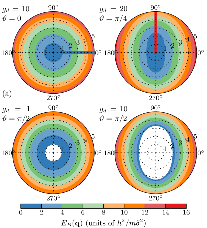
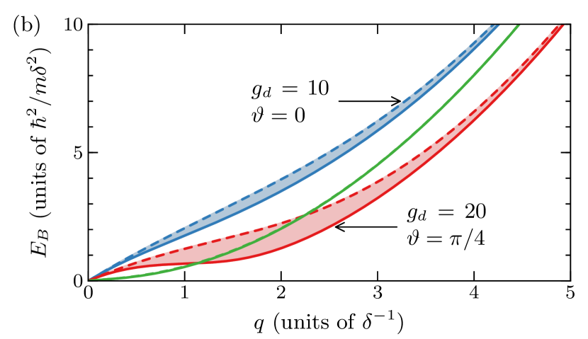
Figure 6: (Color online) Bogoliubov energies for different polarizations and DDI strengths. The polar plots in (a) are marked with the magnitude and angle of $\boldsymbol{\mathrm{q}}$. White areas mark unstable regions. (b): Cuts through Bogoliubov energies at the polar angles indicated in (a). Solid lines include intra- and interlayer DDI, whereas dashed lines only include the intralayer DDI. The green line represents ⁵²Cr. The interlayer DDI does not influence high energies where the in-plane excitations become particle-like. Parameters are as in Fig. 3 with $g=0$ and $\nu=1/10$.

Figure 6 shows the Bogoliubov energy Eq. (20) of a dipole-dominated quasi-2D multilayer BEC for three polarization directions. For nonperpendicular polarizations the Bogoliubov energy becomes anisotropic with higher energies along the projected polarization direction. In Fig. 6 we observe the instability at low momenta for $\vartheta=\pi/2$. The cuts in Fig. 6(b) show the development of a roton minimum at moderately large DDI strength. The interlayer DDI advances the development of this minimum to smaller values of $g_{d}$ compared to a single layer quasi-2D dipolar BEC. For comparison we also plot the Bogoliubov energy for ⁵²Cr in Fig. 6(b), where we assumed that the contact interaction has been reduced to $g=0$ via a Feshbach resonance Koch et al. (2008). The interlayer DDI strength of ⁵²Cr is too weak to influence the dispersion significantly.

VI Conclusion

We showed that interlayer DDI in a multilayer stack of dipolar BECs markedly reduces the aspect ratio of the quasi-2D BEC in the central layer. The greatest change in aspect ratio occurs for parallel polarization. We suggested that this effect of the interlayer DDI is observable in time of flight image of the central layer.

To simplify numerical computations we presented a 2D model for a stack of quasi-2D dipolar BECs created by a strong 1D optical lattice and transversely trapped in a harmonic potential. Our model is based on a dimension reduction of the GPE assuming a Gaussian axial density profile of the wave function in the individual layers. We derived effective intra- and interlayer DDI potentials for the resulting coupled quasi-2D BECs. For weak interlayer DDI we observed only small variations in the particle numbers per lattice site, which allowed us to derive a single mode approximation for the quasi-2D BECs in the central sites. This approximation reduces the numerical computation of mean-field ground states of this system from $\sim 1$ day to several seconds. The resulting ground states match the reduced ground states of the 3D GPE excellently up to moderately large DDI strengths. For large DDI strengths $g_{d}\simeq g$ we still found very good agreement at all polarizations.

Finally, the interlayer DDI reduces the squared Bogoliubov energy, which influences the development of a roton minimum and possibly leads to an instability (imaginary energy) for large density or DDI strength. The excitation spectrum of local perturbations becomes anisotropic for nonperpendicular polarization.

Appendix A Derivation of the effective 2D model

In this appendix we present the derivation of the effective 2D model for multilayered dipolar BECs in a 1D optical lattice [Eq. (5)]. First we use the identity $U_{\text{dd}}(\boldsymbol{\mathrm{r}})=-c_{\text{dd}}[\delta(\boldsymbol{\mathrm{r}})/3+\partial_{\boldsymbol{\mathrm{d}}\boldsymbol{\mathrm{d}}}(1/4\pi|\boldsymbol{\mathrm{r}}|)]$ to split the DDI into a local and nonlocal part O’Dell et al. (2004); Bao et al. (2010). Then we insert $\psi(\boldsymbol{\mathrm{r}},t)=\mathrm{e}^{-\mathrm{i}t/2\gamma^{2}}\sum_{j}\psi_{j}(\boldsymbol{\mathrm{\rho}},t)w_{j}(z)$ with $w_{j}(z)=(1/\pi\gamma^{2})^{1/4}\mathrm{e}^{-(z-z_{j})^{2}/2\gamma^{2}}$ into Eq. (2), where we approximate $V_{o}(z)\simeq\tfrac{1}{2\gamma^{4}}\sum_{j}(z-z_{j})^{2}$. We multiply by $w_{\ell}(z)$ and integrate the resulting equation over $z$. Setting $\int dzw_{\ell}(z)w_{j}(z)=0$ for $\ell\neq j$ and using $\int dzw_{\ell}^{2}(z)=1$, $\int dzw_{\ell}^{4}(z)=1/\sqrt{2\pi\gamma^{2}}$ we find

$$\mathrm{i}\partial_{t}\psi_{\ell}=\left[-\frac{1}{2}\nabla_{\perp}^{2}+V_{\text{ho}}+\bar{g}(1-\epsilon_{\text{dd}})|\psi_{\ell}|^{2}\right]\psi_{\ell}+\Psi_{\ell}.$$ (21)

Here, $\nabla_{\perp}=\partial_{xx}+\partial_{yy}$ and

$$\begin{split}\Psi_{\ell}&=-3g_{d}\int dzd^{3}\boldsymbol{\mathrm{r}}^{\prime}w_{\ell}(z)\partial_{\boldsymbol{\mathrm{d}}\boldsymbol{\mathrm{d}}}U_{\text{3D}}(\boldsymbol{\mathrm{r}}-\boldsymbol{\mathrm{r}}^{\prime})\\ &\quad\times\sum_{j,p,q}\psi_{j}^{*}(\boldsymbol{\mathrm{\rho}}^{\prime},t)\psi_{p}(\boldsymbol{\mathrm{\rho}}^{\prime},t)\psi_{q}(\boldsymbol{\mathrm{\rho}},t)w_{j}(z^{\prime})w_{p}(z^{\prime})w_{q}(z).\end{split}$$ (22)

The kernel in Eq. (22) fulfills $\nabla^{2}U_{\text{3D}}(\boldsymbol{\mathrm{r}})=-\delta(\boldsymbol{\mathrm{r}})$ so that for any $f=f(\boldsymbol{\mathrm{r}})$

$$\partial_{zz}(U_{\text{3D}}\star f)=-f-\nabla_{\perp}^{2}(U_{\text{3D}}\star f),$$ (23)

where $\star$ denotes a convolution. We expand the directional derivative in Eq. (22) as $\partial_{\boldsymbol{\mathrm{d}}\boldsymbol{\mathrm{d}}}=\partial_{\boldsymbol{\mathrm{d}}_{\perp}\boldsymbol{\mathrm{d}}_{\perp}}+d_{z}^{2}\partial_{zz}+2d_{z}\partial_{\boldsymbol{\mathrm{d}}_{\perp}z}$ with $\boldsymbol{\mathrm{d}}_{\perp}=(d_{x},d_{y})$. Applying Eq. (23) to the convolution in Eq. (22) yields

$$\begin{split}\Psi_{\ell}&=3g_{d}\Biggl{(}\frac{d_{z}^{2}}{\sqrt{2\pi\gamma^{2}}}-\sum_{j,p,q}\int dzd^{3}\boldsymbol{\mathrm{r}}^{\prime}\psi_{q}(\boldsymbol{\mathrm{\rho}},t)w_{q}(z)w_{\ell}(z)\\ &\quad\times\bigl{(}\partial_{\boldsymbol{\mathrm{d}}_{\perp}\boldsymbol{\mathrm{d}}_{\perp}}-d_{z}^{2}\nabla_{\perp}^{2}+2d_{z}\partial_{\boldsymbol{\mathrm{d}}_{\perp}z}\bigr{)}U_{\text{3D}}(\boldsymbol{\mathrm{r}}-\boldsymbol{\mathrm{r}}^{\prime})\\ &\quad\times\psi_{j}^{*}(\boldsymbol{\mathrm{\rho}}^{\prime},t)\psi_{p}(\boldsymbol{\mathrm{\rho}}^{\prime},t)w_{j}(z^{\prime})w_{p}(z^{\prime})\Biggr{)}.\end{split}$$ (24)

The first term in Eq. (24) contributes to the contact interaction, whereas the second term forms the nonlocal potential.

The even kernel $U_{\text{even}}^{j\ell}$ [Eq. (6)] is determined by the terms in Eq. (24) with only radial derivatives. After inserting $U_{\text{3D}}$ and the Gaussians $w_{j}$ into Eq. (24), we need to solve the integral

$$\iint dzdz^{\prime}\frac{\mathrm{e}^{-[(z^{\prime}-z_{j})^{2}+(z^{\prime}-z_{p})^{2}+(z-z_{q})^{2}+(z-z_{\ell})^{2}]/2\gamma^{2}}}{4\pi^{2}\gamma^{2}\sqrt{(x-x^{\prime})^{2}+(y-y^{\prime})^{2}+(z-z^{\prime})^{2}}}.$$ (25)

We substitute $\zeta=z-z^{\prime}-(z_{q}+z_{\ell}-z_{j}-z_{p})/2$, $\zeta^{\prime}=z+z^{\prime}-(z_{q}+z_{\ell}+z_{j}+z_{p})/2$ in Eq. (25) and integrate over $\zeta^{\prime}$. The solution defines the even kernel of the DDI potential with $\rho=\sqrt{(x-x^{\prime})^{2}+(y-y^{\prime})^{2}}$

$$U_{\text{even}}^{jpq\ell}(\rho)=\frac{1}{2(2\pi)^{3/2}\gamma}\int d\zeta\frac{\mathrm{e}^{-\zeta^{2}/2\gamma^{2}}\mathrm{e}^{-\bigl{(}\delta_{jp}^{2}+\delta_{q\ell}^{2}\bigr{)}/4\gamma^{2}}}{\sqrt{\rho^{2}+\left(\zeta+\frac{\delta_{qj}+\delta_{\ell p}}{2}\right)^{2}}}.$$ (26)

In Fourier space with $\boldsymbol{\mathrm{k}}=k(\cos\varphi,\sin\varphi)$ the derivatives $\partial_{\boldsymbol{\mathrm{d}}_{\perp}\boldsymbol{\mathrm{d}}_{\perp}}-d_{z}^{2}\nabla_{\perp}^{2}$ in Eq. (24) become $-k^{2}[(d_{x}\cos\varphi+d_{y}\sin\varphi)^{2}-d_{z}^{2}]$. We use the convention $\hat{f}(\boldsymbol{\mathrm{k}})=(1/2\pi)\int d^{2}\boldsymbol{\mathrm{\rho}}f(\boldsymbol{\mathrm{\rho}})\mathrm{e}^{-\mathrm{i}\boldsymbol{\mathrm{k}}\cdot\boldsymbol{\mathrm{\rho}}}$ for the 2D Fourier transform. With this normalization the convolution theorem is $\mathcal{F}[f\star h]=2\pi\mathcal{F}[f]\mathcal{F}[h]$. For radially symmetric $f(\boldsymbol{\mathrm{\rho}})=f(\rho)$: $\hat{f}(k)=\int d\rho\rho f(\rho)J_{0}(k\rho)$ with $J_{0}$ the Bessel function. Using this formula for the Fourier transform of the Eq. (26) and multiplying by $2\pi k^{2}$ from the convolution and the Fourier transform of the derivatives in Eq. (24) we find

$$\begin{split}\hat{U}_{\text{even}}^{jpq\ell}(k)&=\frac{k}{4}\Biggl{[}\eta\left(\frac{\gamma^{2}k+(\delta_{qj}+\delta_{\ell p})/2}{\sqrt{2\gamma^{2}}}\right)\\ &\quad+\eta\left(\frac{\gamma^{2}k-(\delta_{qj}+\delta_{\ell p})/2}{\sqrt{2\gamma^{2}}}\right)\Biggr{]}\\ &\quad\times\mathrm{e}^{-\tfrac{2\delta_{jp}^{2}+2\delta_{q\ell}^{2}+(\delta_{qj}+\delta_{\ell p})^{2}}{8\gamma^{2}}}.\end{split}$$ (27)

For $j=p=q=\ell$ Eq. (27) reduces to the intralayer DDI $\hat{U}_{\text{2D}}(k)$. Because of the exponential prefactor, terms where all $j,p,q,\ell$ are mutually unequal are strongly suppressed. Similarly, terms with $q=j$, $p=\ell$ and $j\neq\ell$ are exponentially suppressed. The remaining terms $q=\ell$, $p=j$, and $j\neq\ell$ form the interlayer DDI kernel $\hat{U}_{\text{even}}^{j\ell}$ [Eq. (6)].

The odd kernel $U_{\text{odd}}^{j\ell}$ [Eq. (7)] is determined by the term in Eq. (24) with derivative $\partial_{\boldsymbol{\mathrm{d}}_{\perp}z}$. Using $\partial_{z}(U_{\text{3D}}\star g)=(\partial_{z}U_{\text{3D}})\star g$ we insert the derivative $\partial_{z}U_{\text{3D}}$ into Eq. (24). Then we need to solve the integral

$$-\iint dzdz^{\prime}\frac{(z-z^{\prime})\mathrm{e}^{-[(z^{\prime}-z_{j})^{2}+(z^{\prime}-z_{p})^{2}+(z-z_{q})^{2}+(z-z_{\ell})^{2}]/2\gamma^{2}}}{4\pi^{2}\gamma^{2}[(x-x^{\prime})^{2}+(y-y^{\prime})^{2}+(z-z^{\prime})^{2}]^{3/2}}.$$ (28)

Following the steps for the even kernel we obtain the odd kernel

$$\begin{split}U_{\text{odd}}^{jpq\ell}(\rho)&=-\frac{1}{2(2\pi)^{3/2}\gamma}\int d\zeta\left(\zeta+\frac{\delta_{qj}+\delta_{\ell p}}{2}\right)\\ &\quad\times\frac{\mathrm{e}^{-\zeta^{2}/2\gamma^{2}}\mathrm{e}^{-\bigl{(}\delta_{jp}^{2}+\delta_{q\ell}^{2}\bigr{)}/4\gamma^{2}}}{\Bigl{[}\rho^{2}+\Bigl{(}\zeta+\frac{\delta_{qj}+\delta_{\ell p}}{2}\Bigr{)}^{2}\Bigr{]}^{3/2}}.\end{split}$$ (29)

The Fourier transform of $U_{\text{odd}}^{jpq\ell}$ [Eq. (29)] multiplied by $2\pi k$ from from the Fourier transforms of the convolution and the remaining radial derivative is given by

$$\begin{split}\hat{U}_{\text{odd}}^{jpq\ell}(k)&=\frac{k}{4}\Biggl{[}\eta\left(\frac{\gamma^{2}k+(\delta_{qj}+\delta_{\ell p})/2}{\sqrt{2\gamma^{2}}}\right)\\ &\quad-\eta\left(\frac{\gamma^{2}k-(\delta_{qj}+\delta_{\ell p})/2}{\sqrt{2\gamma^{2}}}\right)\Biggr{]}\\ &\quad\times\mathrm{e}^{-\tfrac{2\delta_{jp}^{2}+2\delta_{q\ell}^{2}+(\delta_{qj}+\delta_{\ell p})^{2}}{8\gamma^{2}}}.\end{split}$$ (30)

Only terms with $q=\ell$, $p=j$ are not exponentially suppressed in Eq. (30). Hence, we recover $\hat{U}_{\text{odd}}^{j\ell}$ [Eq. (7)].

By combining Eqs. (27) and (30) with Eq. (24) and neglecting the suppressed terms in the sum we recover the DDI potential Eq. (5) in Fourier space.

For completeness we present an approximation of the spatial potential for multilayer DDI with arbitrary polarization direction. To obtain this approximation we take the limit $\gamma\rightarrow 0$ in Eqs. (26) and (29) treat the Gaussians in $\zeta$ as approximations for the Dirac delta distribution:

$$\lim_{\gamma\rightarrow 0}U_{\text{even}}^{j\ell}(\rho) =\frac{1}{4\pi}\frac{1}{\left(\rho^{2}+\delta_{\ell j}^{2}\right)^{1/2}},$$ (31)

$$\lim_{\gamma\rightarrow 0}U_{\text{odd}}^{j\ell}(\rho) =-\frac{1}{4\pi}\frac{\delta_{\ell j}}{\left(\rho^{2}+\delta_{\ell j}^{2}\right)^{3/2}}.$$ (32)

Again we neglect the exponentially suppressed terms. Inserting these kernels into Eq. (24) and calculating the remaining derivatives we find

$$V_{\text{2D}}^{\ell}(\boldsymbol{\mathrm{\rho}})=3g_{d}\sum_{j}\int d\boldsymbol{\mathrm{\rho}}^{\prime}U_{\text{2D}}^{j\ell}(\boldsymbol{\mathrm{\rho}}-\boldsymbol{\mathrm{\rho}}^{\prime})|\psi_{j}(\boldsymbol{\mathrm{\rho}}^{\prime},t)|^{2}$$ (33)

with

$$\begin{split}U_{\text{2D}}^{j\ell}(\boldsymbol{\mathrm{\rho}})&\simeq\frac{1}{4\pi\left(\rho^{2}+\delta_{\ell j}^{2}\right)^{5/2}}\bigl{[}\rho^{2}+(1-3d_{z}^{2})\delta_{\ell j}^{2}\\ &\quad-6d_{z}\delta_{\ell j}\boldsymbol{\mathrm{d}}_{\perp}\cdot\boldsymbol{\mathrm{\rho}}-3|\boldsymbol{\mathrm{d}}_{\perp}\cdot\boldsymbol{\mathrm{\rho}}|^{2}\bigr{]}.\end{split}$$ (34)

For the intralayer part $j=\ell$ this approximation remains valid for $\rho\gg\gamma$. We note that Eq. (34) corresponds to the dimensionless DDI potential Eq. (1) projected onto 2D planes separated by $\delta_{\ell j}$.

References

- Lee et al. (2006) P. A. Lee, N. Nagaosa, and X.-G. Wen, Rev. Mod. Phys. 78, 17 (2006).
- De’Bell et al. (2000) K. De’Bell, A. B. MacIsaac, and J. P. Whitehead, Rev. Mod. Phys. 72, 225 (2000).
- Lahaye et al. (2009) T. Lahaye, C. Menotti, L. Santos, M. Lewenstein, and T. Pfau, Rep. Prog. Phys. 72, 126401 (2009).
- Baranov (2008) M. A. Baranov, Phys. Rep. 464, 71 (2008).
- Góral et al. (2000) K. Góral, K. Rza̧żewski, and T. Pfau, Phys. Rev. A 61, 051601 (2000).
- Yi and You (2000) S. Yi and L. You, Phys. Rev. A 61, 041604 (2000).
- Santos et al. (2000) L. Santos, G. V. Shlyapnikov, P. Zoller, and M. Lewenstein, Phys. Rev. Lett. 85, 1791 (2000).
- Santos et al. (2003) L. Santos, G. V. Shlyapnikov, and M. Lewenstein, Phys. Rev. Lett. 90, 250403 (2003).
- Fischer (2006) U. R. Fischer, Phys. Rev. A 73, 031602 (2006).
- Yi and You (2001) S. Yi and L. You, Phys. Rev. A 63, 053607 (2001).
- Büchler et al. (2007) H. P. Büchler, E. Demler, M. Lukin, A. Micheli, N. Prokof’ev, G. Pupillo, and P. Zoller, Phys. Rev. Lett. 98, 060404 (2007).
- Góral et al. (2002) K. Góral, L. Santos, and M. Lewenstein, Phys. Rev. Lett. 88, 170406 (2002).
- Micheli et al. (2006) A. Micheli, G. K. Brennen, and P. Zoller, Nat. Phys. 2, 341 (2006).
- Griesmaier et al. (2005) A. Griesmaier, J. Werner, S. Hensler, J. Stuhler, and T. Pfau, Phys. Rev. Lett. 94, 160401 (2005).
- Stuhler et al. (2005) J. Stuhler, A. Griesmaier, T. Koch, M. Fattori, T. Pfau, S. Giovanazzi, P. Pedri, and L. Santos, Phys. Rev. Lett. 95, 150406 (2005).
- Koch et al. (2008) T. Koch, T. Lahaye, J. Metz, B. Fröhlich, A. Griesmaier, and T. Pfau, Nat. Phys. 4, 218 (2008).
- Berglund et al. (2008) A. J. Berglund, J. L. Hanssen, and J. J. McClelland, Phys. Rev. Lett. 100, 113002 (2008).
- Lu et al. (2010) M. Lu, S. H. Youn, and B. L. Lev, Phys. Rev. Lett. 104, 063001 (2010).
- Fattori et al. (2008) M. Fattori, G. Roati, B. Deissler, C. D’Errico, M. Zaccanti, M. Jona-Lasinio, L. Santos, M. Inguscio, and G. Modugno, Phys. Rev. Lett. 101, 190405 (2008).
- Vengalattore et al. (2008) M. Vengalattore, S. R. Leslie, J. Guzman, and D. M. Stamper-Kurn, Phys. Rev. Lett. 100, 170403 (2008).
- Vogt et al. (2006) T. Vogt, M. Viteau, J. Zhao, A. Chotia, D. Comparat, and P. Pillet, Phys. Rev. Lett. 97, 083003 (2006).
- Ni et al. (2010) K. Ni, S. Ospelkaus, D. Wang, G. Quemener, B. Neyenhuis, M. H. G. de Miranda, J. L. Bohn, J. Ye, and D. S. Jin, Nature 464, 1324 (2010).
- de Miranda et al. (2011) M. H. G. de Miranda, A. Chotia, B. Neyenhuis, D. Wang, G. Quemener, S. Ospelkaus, J. L. Bohn, J. Ye, and D. S. Jin, Nat. Phys. 7, 502 (2011).
- Voigt et al. (2009) A. Voigt, M. Taglieber, L. Costa, T. Aoki, W. Wieser, T. W. Hänsch, and K. Dieckmann, Phys. Rev. Lett. 102, 020405 (2009).
- Müller et al. (2011) S. Müller, J. Billy, E. A. L. Henn, H. Kadau, A. Griesmaier, M. Jona-Lasinio, L. Santos, and T. Pfau, (2011), arXiv:1105.5015 .
- Klawunn et al. (2010) M. Klawunn, A. Pikovski, and L. Santos, Phys. Rev. A 82, 044701 (2010).
- Baranov et al. (2011) M. A. Baranov, A. Micheli, S. Ronen, and P. Zoller, Phys. Rev. A 83, 043602 (2011).
- Shih and Wang (2009) S.-M. Shih and D.-W. Wang, Phys. Rev. A 79, 065603 (2009).
- Potter et al. (2010) A. C. Potter, E. Berg, D.-W. Wang, B. I. Halperin, and E. Demler, Phys. Rev. Lett. 105, 220406 (2010).
- Rosenkranz and Bao (2011) M. Rosenkranz and W. Bao, “Scattering and bound states in two-dimensional anisotropic potentials,” (2011), in preparation.
- Volosniev et al. (2011a) A. G. Volosniev, D. V. Fedorov, A. S. Jensen, and N. T. Zinner, Phys. Rev. Lett. 106, 250401 (2011a).
- Bao and Tang (2003) W. Bao and W. J. Tang, J. Comput. Phys. 187, 230 (2003).
- Bao et al. (2003) W. Bao, D. Jaksch, and P. A. Markowich, J. Comput. Phys. 187, 318 (2003).
- Salasnich (2009) L. Salasnich, J. Phys. A: Math. Theor. 42, 335205 (2009).
- Abdallah et al. (2005) N. B. Abdallah, F. Méhats, C. Schmeiser, and R. Weishäupl, SIAM J. Math. Anal. 37, 189 (2005).
- Abdallah et al. (2008) N. B. Abdallah, F. Castella, and F. Méhats, J. Differential Equations 245, 154 (2008).
- Lieb et al. (2003) E. H. Lieb, R. Seiringer, and J. Yngvason, Phys. Rev. Lett. 91, 150401 (2003).
- Yngvason et al. (2004) J. Yngvason, E. H. Lieb, and R. Seiringer, Commun. Math. Phys. 244, 347 (2004).
- Carles et al. (2008) R. Carles, P. A. Markowich, and C. Sparber, Nonlinearity 21, 2569 (2008).
- Cai et al. (2010) Y. Cai, M. Rosenkranz, Z. Lei, and W. Bao, Phys. Rev. A 82, 043623 (2010).
- Pitaevskii and Stringari (2003) L. Pitaevskii and S. Stringari, Bose-Einstein Condensation (Oxford University Press, Oxford, 2003).
- Giovanazzi et al. (2002) S. Giovanazzi, A. Görlitz, and T. Pfau, Phys. Rev. Lett. 89, 130401 (2002).
- Marinescu and You (1998) M. Marinescu and L. You, Phys. Rev. Lett. 81, 4596 (1998).
- Deb and You (2001) B. Deb and L. You, Phys. Rev. A 64, 022717 (2001).
- Burger et al. (2002) S. Burger, F. S. Cataliotti, C. Fort, P. Maddaloni, F. Minardi, and M. Inguscio, EPL 57, 1 (2002).
- Petrov et al. (2000) D. S. Petrov, M. Holzmann, and G. V. Shlyapnikov, Phys. Rev. Lett. 84, 2551 (2000).
- Volosniev et al. (2011b) A. G. Volosniev, N. T. Zinner, D. V. Fedorov, A. S. Jensen, and B. Wunsch, J. Phys. B 44, 125301 (2011b).
- Bao et al. (2010) W. Bao, Y. Cai, and H. Wang, J. Comput. Phys. 229, 7874 (2010).
- Bao (2004) W. Bao, Multiscale Modeling and Simulation: a SIAM Interdisciplinary Journal 2, 210 (2004).
- Bao and Du (2004) W. Bao and Q. Du, SIAM J. Sci. Comput. 25, 1674 (2004).
- Lahaye et al. (2007) T. Lahaye, T. Koch, B. Fröhlich, M. Fattori, J. Metz, A. Griesmaier, S. Giovanazzi, and T. Pfau, Nature 448, 672 (2007).
- Rosenkranz and Fischer (2011) M. Rosenkranz and U. R. Fischer, “Instabilities in quasi-2D dipolar Bose-Einstein condensates,” (2011), in preparation.
- O’Dell et al. (2004) D. H. J. O’Dell, S. Giovanazzi, and C. Eberlein, Phys. Rev. Lett. 92, 250401 (2004).