$\bf M_{h}$ in the MSSM-seesaw scenario with ILC precision

Abstract

We review the computation of the one-loop radiative corrections from the neutrino/ sneutrino sector to the lightest Higgs boson mass, $M_{h}$, within the context of the so-called MSSM-seesaw scenario. This model introduces right handed neutrinos and their supersymmetric partners, the sneutrinos, including Majorana mass terms. We find negative and sizeable corrections to $M_{h}$, up to $-5\,\,\mathrm{GeV}$ for a large Majorana scale, $10^{13}-10^{15}\,\,\mathrm{GeV}$, and for the lightest neutrino mass in a range $0.1-1$ eV. The corrections to $M_{h}$ are substantially larger than the anticipated ILC precision for large regions of the MSSM-seesaw parameter space.

1 Introduction

The current experimental data on neutrino mass differences and neutrino mixing angles clearly indicate new physics beyond the so far successful Standard Model (SM) of Particle Physics. In particular, neutrino oscillations imply that at least two generations of neutrinos must be massive. Therefore, one needs to extend the SM to incorporate neutrino mass terms.

We have explored [1] the simplest version of a Supersymmetric extension of the SM, the well known Minimal Supersymmetric Standard Model (MSSM), extended by right-handed Majorana neutrinos and where the seesaw mechanism of type I [2] is implemented to generate the small neutrino masses. For simplicity, as a first step, we focus here in the one generation case.

On the other hand, it is well known that heavy Majorana neutrinos, with a Majorana mass scale $m_{M}\sim 10^{13}-10^{15}\,\,\mathrm{GeV}$, induce large LFV rates [3], due to their potentially large Yukawa couplings to the Higgs sector. For the same reason, radiative corrections to Higgs boson masses due to such heavy Majorana neutrinos could also be relevant. Consequently, our study has been focused on the radiative corrections to the lightest MSSM ${\cal CP}$-even $h$ boson mass, $M_{h}$, due to the one-loop contributions from the neutrino/sneutrino sector within the MSSM-seesaw framework.

In the following we briefly review the main relevant aspects of the calculation of the mass corrections and the numerical results. Further details can be found in [1], where also an extensive list with references to previous works can be found.

2 The MSSM-seesaw model

The MSSM-seesaw model with one neutrino/sneutrino generation is described in terms of the well known MSSM superpotential plus the new relevant terms given as:

$$W\,=\,\epsilon_{ij}\left[Y_{\nu}\hat{H}_{2}^{i}\,\hat{L}^{j}\hat{N}\,-\,Y_{l}\hat{H}_{1}^{i}\,\hat{L}^{j}\,\hat{R}\right]\,+\,\frac{1}{2}\,\hat{N}\,m_{M}\,\hat{N}\,,$$ (1)

where $\hat{N}=(\tilde{\nu}_{R}^{*},(\nu_{R})^{c})$ is the additional superfield that contains the right-handed neutrino $\nu_{R}$ and its scalar partner $\tilde{\nu}_{R}$.

There are also new relevant terms in the soft SUSY breaking potential:

$$V^{\tilde{\nu}}_{\rm soft}=m^{2}_{\tilde{L}}\tilde{\nu}_{L}^{*}\tilde{\nu}_{L}+m^{2}_{\tilde{R}}\tilde{\nu}_{R}^{*}\tilde{\nu}_{R}+(Y_{\nu}A_{\nu}H^{2}_{2}\tilde{\nu}_{L}\tilde{\nu}_{R}^{*}+m_{M}B_{\nu}\tilde{\nu}_{R}\tilde{\nu}_{R}+{\rm h.c.})~{}.$$ (2)

After electro-weak (EW) symmetry breaking, the charged lepton and Dirac neutrino masses can be written as

$$m_{l}\,=\,Y_{l}\,\,v_{1}\,,\quad\quad m_{D}\,=\,Y_{\nu}\,v_{2}\,,$$ (3)

where $v_{i}$ are the vacuum expectation values (VEVs) of the neutral Higgs scalars, with $v_{1(2)}=\,v\,\cos(\sin)\beta$ and $v\simeq 174\,\,\mathrm{GeV}$.

The $2\times 2$ neutrino mass matrix is given in terms of $m_{D}$ and $m_{M}$ by:

$$M^{\nu}\,=\,\left(\begin{array}[]{cc}0&m_{D}\\ m_{D}&m_{M}\end{array}\right)\,.$$ (4)

Diagonalization of $M^{\nu}$ leads to two mass eigenstates, which are Majorana fermions with the respective mass eigenvalues given by:

$$m_{\nu,\,N}=\frac{1}{2}\left(m_{M}\mp\sqrt{m_{M}^{2}+4m_{D}^{2}}\right)~{}.$$ (5)

In the seesaw limit, i.e. when $\xi\equiv\frac{m_{D}}{m_{M}}\ll 1~{}$, one finds,

$$m_{\nu}=-m_{D}\xi+\mathcal{O}(m_{D}\xi^{3})\simeq-\frac{m_{D}^{2}}{m_{M}}~{},\quad\quad m_{N} =m_{M}+\mathcal{O}(m_{D}\xi)\simeq m_{M}~{}.$$ (6)

Regarding the sneutrino sector, the sneutrino mass matrices for the ${\cal CP}$-even, ${\tilde{M}}_{+}$, and the ${\cal CP}$-odd, ${\tilde{M}}_{-}$, subsectors are given respectively by

$${\tilde{M}}_{\pm}^{2}=\left(\begin{array}[]{cc}m_{\tilde{L}}^{2}+m_{D}^{2}+\frac{1}{2}M_{Z}^{2}\cos 2\beta&m_{D}(A_{\nu}-\mu\cot\beta\pm m_{M})\\ m_{D}(A_{\nu}-\mu\cot\beta\pm m_{M})&m_{\tilde{R}}^{2}+m_{D}^{2}+m_{M}^{2}\pm 2B_{\nu}m_{M}\end{array}\right)~{}.$$ (7)

The diagonalization of these two matrices, ${\tilde{M}}_{\pm}^{2}$, leads to four sneutrino mass eigenstates. In the seesaw limit, where $m_{M}$ is much bigger than all the other scales the corresponding sneutrino masses are given by:

$$m_{{\tilde{\nu}_{+}},{\tilde{\nu}_{-}}}^{2} = m_{\tilde{L}}^{2}+\frac{1}{2}M_{Z}^{2}\cos 2\beta\mp 2m_{D}(A_{\nu}-\mu\cot\beta-B_{\nu})\xi~{},$$

$$m_{{\tilde{N}_{+}},{\tilde{N}_{-}}}^{2} = m_{M}^{2}\pm 2B_{\nu}m_{M}+m_{\tilde{R}}^{2}+2m_{D}^{2}~{}.$$ (8)

Finally, in the interaction Lagrangian that is relevant for the present work, there are terms already present in the MSSM: the pure gauge interactions between the left-handed neutrinos and the $Z$ boson, those between the ’left-handed’ sneutrinos and the Higgs bosons, and those between the ’left-handed’ sneutrinos and the $Z$ bosons. In addition, in this MSSM-seesaw scenario, there are interactions driven by the neutrino Yukawa couplings (or equivalently $m_{D}$ since $Y_{\nu}=(gm_{D})/(\sqrt{2}M_{W}\sin\beta)$), as for instance $g_{h\nu_{L}\nu_{R}}=-\frac{igm_{D}\cos\alpha}{2M_{W}\sin\beta}$, and new interactions due to the Majorana nature driven by $m_{M}$, which are not present in the case of Dirac fermions, as for instance $g_{h\tilde{\nu}_{L}\tilde{\nu}_{R}}=-\frac{igm_{D}m_{M}\cos\alpha}{2M_{W}\sin\beta}$. Besides, the Higgs boson sector in the MSSM-seesaw model is as in the MSSM.

3 Calculation

In the Feynman diagrammatic (FD) approach the higher-order corrected ${\cal CP}$-even Higgs boson masses in the MSSM, denoted here as $M_{h}$ and $M_{H}$, are derived by finding the poles of the $(h,H)$-propagator matrix, which is equivalent to solving the following equation [4]:

$$\left[p^{2}-m_{h}^{2}+\hat{\Sigma}_{hh}(p^{2})\right]\left[p^{2}-m_{H}^{2}+\hat{\Sigma}_{HH}(p^{2})\right]-\left[\hat{\Sigma}_{hH}(p^{2})\right]^{2}=0~{},$$ (9)

where $m_{h,H}$ are the tree level masses. The one loop renormalized self-energies, $\hat{\Sigma}_{\phi\phi}(p^{2})$, in (9) can be expressed in terms of the bare self-energies, $\Sigma_{\phi\phi}(p^{2})$, the field renormalization constants $\delta Z_{\phi\phi}$ and the mass counter terms $\delta m_{\phi}^{2}$, where $\phi$ stands for $h,H$. For example, the lightest Higgs boson renormalized self energy reads:

$$\hat{\Sigma}_{hh}(p^{2})=\Sigma_{hh}(p^{2})+\delta Z_{hh}(p^{2}-m_{h}^{2})-\delta m_{h}^{2}~{}.$$ (10)

Regarding the renormalization prescription, we have used an on-shell renormalization scheme for $M_{Z},M_{W}$ and $M_{A}$ mass counterterms and $T_{h},T_{H}$ tadpole counterterms. On the other hand, we have used a modified $\overline{\mathrm{DR}}$ scheme $\left(\mathrm{m}\overline{\mathrm{DR}}\right)$ for the renormalization of the wave function and $\tan\beta\,$. The m$\overline{\mathrm{DR}}$ scheme is very similar to the well known $\overline{\mathrm{DR}}$ scheme but instead of subtracting the usual term proportional to $\Delta=\frac{2}{\epsilon}-\gamma_{E}+\log(4\pi)$ one subtracts the term proportional to $\Delta_{m}=\Delta-\log(m^{2}_{M}/\mu^{2}_{\overline{\mathrm{DR}}})$, hence, avoiding large logarithms of the large scale $m_{M}$. As studied in other works [5], this scheme minimizes higher order corrections when two very different scales are involved in a calculation of radiative corrections.

The full one-loop $\nu/\tilde{\nu}$ corrections to the self-energies, $\hat{\Sigma}_{hh}^{\nu/\tilde{\nu}}$, $\hat{\Sigma}_{HH}^{\nu/\tilde{\nu}}$ and $\hat{\Sigma}_{hH}^{\nu/\tilde{\nu}}$, entering (9) have been evaluated with FeynArts  and FormCalc [6]. The new Feynman rules for the $\nu/\tilde{\nu}$ sector are inserted into a new model file. Since we are interested in exploring the relevance of the new radiative corrections to $M_{h}$ from the neutrino/sneutrino sector, we will present here our results in terms of the mass difference with respect to the MSSM prediction. Consequently, we define,

$$\Delta m_{h}^{\mathrm{m}\overline{\mathrm{DR}}}:=M_{h}^{\nu/\tilde{\nu}}-M_{h},$$ (11)

where $M_{h}^{\nu/\tilde{\nu}}$ denotes the pole for the light Higgs mass including the $\nu/\tilde{\nu}$ corrections (i.e. in the MSSM-seesaw model), and $M_{h}$ the corresponding pole in the MSSM, i.e without the $\nu/\tilde{\nu}$ corrections. Thus, for a given set of input parameters we first calculate $M_{h}$ in the MSSM with the help of FeynHiggs [7], such that all relevant known higher-order corrections are included. Then we add the new contributions from the neutrino/sneutrino sector and eventually compute $\Delta m_{h}^{\mathrm{m}\overline{\mathrm{DR}}}$.

4 Results

We have obtained the full analytical results for the renormalized Higgs boson self-energies and their expressions in the seesaw limit. In order to understand in simple terms the analytical behavior of our full numerical results we have expanded the renormalized self-energies in powers of the seesaw parameter $\xi=m_{D}/m_{M}$:

$$\hat{\Sigma}(p^{2})=\left(\hat{\Sigma}(p^{2})\right)_{m_{D}^{0}}+\left(\hat{\Sigma}(p^{2})\right)_{m_{D}^{2}}+\left(\hat{\Sigma}(p^{2})\right)_{m_{D}^{4}}+\ldots~{}.$$ (12)

The zeroth order of this expansion is precisely the pure gauge contribution and it does not depend on $m_{D}$ or $m_{M}$. Therefore, it corresponds to the result in the MSSM. The rest of the terms of the expansion are the Yukawa contribution. The leading term of this Yukawa contribution is the ${\cal O}(m_{D}^{2})$ term, because it is the only one not suppressed by the Majorana scale. In fact it goes as $Y_{\nu}^{2}M^{2}_{\rm EW}$, where $M^{2}_{\rm EW}$ denotes generically the electroweak scales involved, concretely, $p^{2}$, $M_{Z}^{2}$ and $M_{A}^{2}$. In particular, the ${\cal O}(p^{2}m_{D}^{2})$ terms of the renormalized self-energy, which turn out to be the most relevant leading contributions, separated into the neutrino and sneutrino contributions, read:

$$\left.\hat{\Sigma}_{hh}^{\mathrm{m}\overline{\mathrm{DR}}}\right|_{m_{D}^{2}p^{2}}\sim\left.\begin{array}[]{c}\begin{picture}(70.0,40.0) \put(0.0,0.0){} \raise 25.0pt\hbox to0.0pt{\kern 8.0pt\makebox(0.0,0.0)[r]{$h$}\hss} \ignorespaces \put(0.0,0.0){} \raise 25.0pt\hbox to0.0pt{\kern 72.0pt\makebox(0.0,0.0)[l]{$h\,+$}\hss} \ignorespaces \put(0.0,0.0){} \raise 46.0pt\hbox to0.0pt{\kern 40.0pt\makebox(0.0,0.0)[b]{$\nu_{L}$}\hss} \ignorespaces \put(0.0,0.0){} \raise 4.0pt\hbox to0.0pt{\kern 40.0pt\makebox(0.0,0.0)[t]{$\nu_{R}$}\hss} \ignorespaces \end{picture}\end{array}\mbox{~{}~{}}\begin{array}[]{c}\begin{picture}(70.0,40.0) \put(0.0,0.0){} \raise 25.0pt\hbox to0.0pt{\kern 8.0pt\makebox(0.0,0.0)[r]{$h$}\hss} \ignorespaces \put(0.0,0.0){} \raise 25.0pt\hbox to0.0pt{\kern 72.0pt\makebox(0.0,0.0)[l]{$h$}\hss} \ignorespaces \put(0.0,0.0){} \raise 46.0pt\hbox to0.0pt{\kern 40.0pt\makebox(0.0,0.0)[b]{$\tilde{\nu}_{L}$}\hss} \ignorespaces \put(0.0,0.0){} \raise 4.0pt\hbox to0.0pt{\kern 40.0pt\makebox(0.0,0.0)[t]{$\tilde{\nu}_{R}$}\hss} \ignorespaces \end{picture}\end{array}\,\,\right|_{m_{D}^{2}p^{2}}\sim\frac{g^{2}p^{2}m_{D}^{2}c^{2}_{\alpha}}{64\pi^{2}M_{W}^{2}s^{2}_{\beta}}+\frac{g^{2}p^{2}m_{D}^{2}c^{2}_{\alpha}}{64\pi^{2}M_{W}^{2}s^{2}_{\beta}}.$$ (13)

Notice that the above neutrino contributions come from the Yukawa interaction $g_{h\nu_{L}\nu_{R}}$, which is extremely suppressed in the Dirac case but can be large in the Majorana case. The sneutrino contributions come from the new couplings $g_{h\tilde{\nu}_{L}\tilde{\nu}_{R}}$, which are not present in the Dirac case. It is also interesting to remark that these terms, being $\sim p^{2}$, depend on the external momentum. Therefore, at large $m_{M}$, to keep just the Yukawa part is a good approximation, but to neglect the momentum dependence or to set the external momentum to zero are certainly not. In consequence, the effective potential method will not provide a realistic result for the radiative corrections to the Higgs mass. Similarly, obtaining the leading logarithmic terms in a RGE computation, would also miss these finite terms.

The behaviour of the renormalized self-energy with all others parameters entering in the computation have been discussed in [1]. According to our detailed analysis in this paper, the most relevant parameters for our purposes are: $m_{M}$ (or, equivalently, the heaviest physical Majorana neutrino mass $m_{N}$), $m_{\nu}$ and the soft SUSY breaking parameters $m_{\tilde{R}}$ and $B_{\nu}$. In the literature it is often assumed that $m_{M}$ has a very large value, $m_{M}\sim{\cal O}(10^{14-15})\,\,\mathrm{GeV}$, in order to get $|m_{\nu}|\sim$ 0.1 - 1 eV with large Yukawa couplings $Y_{\nu}\sim{\cal O}(1)$. This is an interesting possibility since it can lead to important phenomenological implications due to the large size of the radiative corrections driven by these large $Y_{\nu}$. We have explored, however, not only these extreme values but the full range for $m_{M}$: $\sim 10^{2}-10^{15}\,\,\mathrm{GeV}$.

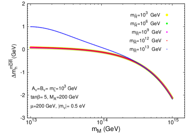
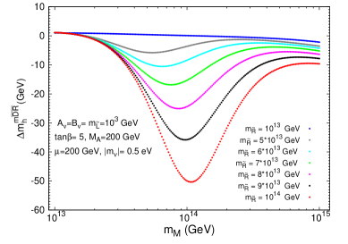
Figure 1: One-loop corrections to $M_{h}$ from the neutrino/sneutrino sector as a function of $m_{M}$ for: ${m_{\tilde{R}}}<10^{13}\,\,\mathrm{GeV}$ (left panel) and $10^{13}\,\,{\rm GeV}<{m_{\tilde{R}}}<10^{14}\,\,{\rm GeV}$ (right panel).

Fig. 1 shows the predictions for $\Delta m_{h}^{\mathrm{m}\overline{\mathrm{DR}}}$ as a function of $m_{M}$, for several input $m_{\tilde{R}}$ values. The Higgs mass corrections are positive and below 0.1 GeV if $m_{M}\;\raisebox{-3.00003pt}{$\stackrel{{\scriptstyle\displaystyle<}}{{\sim}}$}\;5\times 10^{13}\,\,\mathrm{GeV}$ and $m_{\tilde{R}}<10^{12}\,\,\mathrm{GeV}$ (left panel). For larger Majorana mass values, the corrections get negative and grow up to a few GeV; $\Delta m_{h}^{\mathrm{m}\overline{\mathrm{DR}}}=-2.15$ GeV for $m_{M}=10^{15}\,\,\mathrm{GeV}$. The results in the right plot show that for larger values of the soft mass, $m_{\tilde{R}}\;\raisebox{-3.00003pt}{$\stackrel{{\scriptstyle\displaystyle>}}{{\sim}}$}\;10^{13}\,\,\mathrm{GeV}$, the Higgs mass corrections are negative and can be sizeable, a few tens of GeV, reaching their maximum values at $m_{\tilde{R}}\simeq m_{M}$.

The results of the Higgs mass corrections in terms of the two relevant physical Majorana neutrino masses, light $|m_{\nu}|$ and heavy $m_{N}$, are summarized in the left plot of Fig. 2. For values of $m_{N}<3\times 10^{13}$ GeV and $|m_{\nu}|<0.1-0.3$ eV the corrections to $M_{h}$ are positive and smaller than 0.1 GeV. In this region, the gauge contribution dominates. In fact, the wider black contour line with fixed $\Delta m_{h}^{\mathrm{m}\overline{\mathrm{DR}}}=0.09$ coincides with the prediction for the case where just the gauge part in the self-energies have been included. This means that ’the distance’ of any other contour-line respect to this one represents the difference in the radiative corrections respect to the MSSM prediction. For larger values of $m_{N}$ and/or $|m_{\nu}|$ the Yukawa part dominates, and the radiative corrections become negative and larger in absolute value, up to about $-5\,\,\mathrm{GeV}$ in the right upper corner of this figure. These corrections grow in modulus proportionally to $m_{M}$ and $m_{\nu}$, due to the fact that the seesaw mechanism impose a relation between the three masses involved, $m_{D}^{2}=|m_{\nu}|m_{N}$.

Finally, we present in the right plot of Fig. 2 the contour-lines for fixed $\Delta m_{h}^{\mathrm{m}\overline{\mathrm{DR}}}$ in the less conservative case where $m_{\tilde{R}}$ is close to $m_{M}$. These are displayed as a function of $|m_{\nu}|$ and the ratio $m_{\tilde{R}}/m_{M}$. $m_{M}$ is fixed to $10^{14}$ GeV. For the interval studied here, we see again that the radiative corrections can be negative and as large as tens of GeV in the upper right corner of the plot. For instance, $\Delta m_{h}^{\mathrm{m}\overline{\mathrm{DR}}}=-30\,\,\mathrm{GeV}$ for $|m_{\nu}|=0.6$ eV and $m_{\tilde{R}}/m_{M}=0.7$.

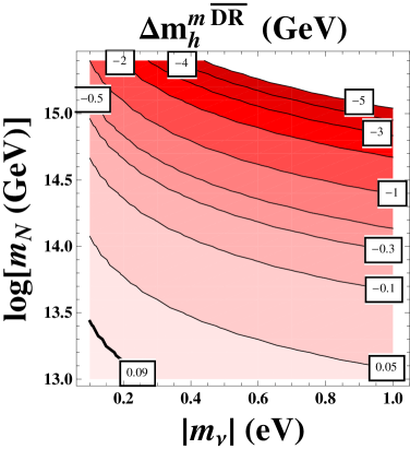
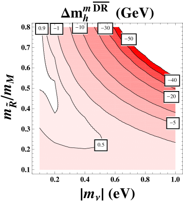
Figure 2: Contour-lines for the Higgs mass corrections from the $\nu/\tilde{\nu}$ sector as a function of: $|m_{\nu}|$ and $m_{N}$ (left panel) and the ratio $m_{\tilde{R}}/m_{M}$ and $|m_{\nu}|$ (right panel). The other parameters are: $A_{\nu}=B_{\nu}=m_{\tilde{L}}=m_{\tilde{R}}=10^{3}\,\,\mathrm{GeV},\tan\beta=5,M_{A}=200\,\,\mathrm{GeV},\mu=200\,\,\mathrm{GeV}$.

To summarize: for some regions of the MSSM-seesaw parameter space, the corrections to $M_{h}$ are of the order of several GeV. For all soft SUSY-breaking parameters at the TeV scale we find correction of up to $-5\,\,\mathrm{GeV}$ to $M_{h}$. These corrections are substantially larger than the anticipated ILC precision of about $50\,\,\mathrm{MeV}$ (and also larger than the anticipated LHC precision of $\sim 200\,\,\mathrm{MeV}$). Consequently, they should be included in any phenomenological analysis of the Higgs sector in the MSSM-seesaw.

References

- [1] S. Heinemeyer, M. J. Herrero, S. Penaranda and A. M. Rodriguez-Sanchez, JHEP 1105 (2011) 063 [arXiv:1007.5512 [hep-ph]].
- [2] P. Minkowski, Phys. Lett. B 67 (1977) 421;
-
[3]
F. Borzumati and A. Masiero,
Phys. Rev. Lett. 57 (1986) 961;
M. Raidal et al., Eur. Phys. J. C 57, 13 (2008) [arXiv:0801.1826 [hep-ph]]. - [4] M. Frank, T. Hahn, S. Heinemeyer, W. Hollik, H. Rzehak and G. Weiglein, JHEP 0702 (2007) 047 [arXiv:0611326 [hep-ph]].
- [5] J. Collins, F. Wilczek and A. Zee, Phys. Rev. D 18 (1978) 242.
-
[6]
J. Küblbeck, M. Böhm and A. Denner,
Comput. Phys. Commun. 60 (1990) 165;
T. Hahn, Comput. Phys. Commun. 140 (2001) 418 [arXiv:hep-ph/0012260];
T. Hahn and C. Schappacher, Comput. Phys. Commun. 143 (2002) 54 [arXiv:hep-ph/0105349];
T. Hahn and M. Pérez-Victoria, Comput. Phys. Commun. 118 (1999) 153 [arXiv:hep-ph/9807565]. - [7] S. Heinemeyer, W. Hollik and G. Weiglein, Comput. Phys. Commun. 124 (2000) 76 [arXiv:hep-ph/9812320]; see: www.feynhiggs.de .