Spin-to-orbital angular momentum conversion and spin-polarization filtering in electron beams

Abstract

We propose the design of a space-variant Wien filter for electron beams that induces a spin half-turn and converts the corresponding spin angular momentum variation into orbital angular momentum (OAM) of the beam itself, by exploiting a geometrical phase arising in the spin manipulation. When applied to a spatially-coherent input spin-polarized electron beam, such device can generate an electron vortex beam, carrying OAM. When applied to an unpolarized input beam, the proposed device in combination with a suitable diffraction element can act as a very effective spin-polarization filter. The same approach can be also applied to neutron or atom beams.

Phase vortices in electronic quantum states have been widely investigated in condensed matter, for example in connection with superconductivity, the Hall effect, etc. Only very recently, however, free-space electron beams exhibiting controlled phase vortices have been experimentally generated in transmission electron microscope (TEM) systems, using either a spiral phase plate obtained from a stack of graphite thin films Uchida and Tonomura (2010), or a “pitchfork” hologram manufactured by ion beam lithography Verbeeck et al. (2010); McMorran et al. (2011). In a cylindrical coordinate system $r,\phi,z$ with the $z$ axis along the beam axis, a vortex electron beam is described by a wavefunction having the general form $\psi(r,\phi,z,t)=u(r,z,t)\exp(i\ell\phi)$, where $\ell$ is a (nonzero) integer and $u$ vanishes at $r=0$. As in the case of atomic orbitals, $\ell$ is the eigenvalue of the $z$-component orbital angular momentum (OAM) operator $\hat{L}_{z}=-i\partial_{\phi}$ (in units of the reduced Planck constant $\hbar$), and therefore an electron beam of this form carries $\ell\hbar$ of OAM per electron Bliokh et al. (2007). The recent experiments on electron vortex beams were inspired by the singular optics field, in which similar phase or holographic tools have been used in the last twenty years (see, e.g., Franke-Arnold et al. (2008) and references therein). In optics, a recently introduced alternative approach to the generation of vortex beams is based on the “conversion” of the angular momentum variation occurring in a spin-flip process into orbital angular momentum of the light beam, when the latter is propagating through a suitable spatially variant birefringent plate Marrucci et al. (2006, 2011). In this paper, we propose that a beam of electrons traveling in free space undergoes a similar “spin-to-orbital angular momentum conversion” (STOC) process in the presence of a suitable space-variant magnetic field. The same approach may work also for neutrons, or any other particle endowed with a spin magnetic moment (e.g., atoms, ions). Of course, in the case of electrons, as for other charged particles, the magnetic field, besides acting on the spin, will also induce forces that must be compensated in order to avoid strong beam distortions or deflections. Such compensation may be obtained by a suitable electric field, and this leads us to conceiving the proposed apparatus essentially as a space-variant Wien filter. Such apparatus can be exploited for generating vortex electron beams when a spin-polarized beam is used as input. Conversely, if a pure vortex beam is used in input, by means e.g. of a holographic method, one can use the STOC process for filtering a single spin-polarized component of the input beam, as we will show further below.

Let us consider an electron beam propagating in vacuum along the $z$-axis and crossing a region of space lying between $z=0$ and $z=L$ in which it is subject to electric and magnetic fields $\bm{E}=-\nabla\Phi$ and $\bm{B}=\nabla\times\bm{A}$, where $\Phi$ and $\bm{A}$ are the scalar and vector potentials, respectively. In the non-relativistic approximation and neglecting all Coulomb self-interaction effects (small charge density limit), the electron beam quantum propagation and spin evolution are generally described by Pauli’s equation

$$i\hbar\partial_{t}\tilde{\psi}=\left[\frac{1}{2m}(-i\hbar\bm{\nabla}-e\bm{A})^{2}+e\Phi-\bm{B}\cdot\hat{\bm{\mu}}\right]\tilde{\psi}$$ (1)

where $\tilde{\psi}$ is the spinorial two-component wave-function of the electron beam, $e=-|e|$ and $m$ are the electron charge and mass, $\partial_{t}$ is the derivative with respect to the time variable $t$, $\hat{\bm{\mu}}=-\frac{1}{2}g\mu_{B}\hat{\bm{\sigma}}$ is the electron magnetic moment, with $\mu_{B}=\hbar|e|/2m$ the Bohr’s magneton, $g\simeq 2$ the electron $g$-factor, and $\hat{\bm{\sigma}}=(\hat{\sigma}_{x},\hat{\sigma}_{y},\hat{\sigma}_{z})$ the Pauli matrix vector.

As a first step, we consider the simpler case in which the electric and magnetic fields are taken to be uniform, lying in the transverse plane $xy$, and arranged as in standard Wien filters Tioukine and Aulenbacher (2006); Grames et al. (2011), i.e. perpendicular to each other and balanced so as to cancel the average Lorentz force, i.e. $E_{0}=B_{0}p_{c}/m$ where $E_{0}$ and $B_{0}$ are the electric and magnetic field moduli, and $p_{c}$ the average beam momentum. The magnetic field $\bm{B}$ is also taken to form an arbitrary angle $\alpha$ with the axis $x$ within the $xy$ plane. For this case, we solved the full Pauli’s equation in the paraxial slow-varying-envelope approximation for an input beam having a gaussian profile and an arbitrary uniform input spin state $|\psi\rangle_{in}=a_{1}|\!\uparrow\rangle+a_{2}|\!\downarrow\rangle$, where $|\!\uparrow\rangle$ and $|\!\downarrow\rangle$ denote a state for which the spin is parallel or antiparallel to the $z$ axis, respectively. The complete expression of the resulting spinorial wave-function is given in the supplemental material (SM) suppl , while here we summarize the main findings. The beam propagation behavior corresponds to the well known astigmatic lensing in the plane perpendicular to the magnetic field. More precisely, the beam undergoes periodic width oscillations, with a spatial period $\Lambda_{2}=\pi R_{c}$, where $R_{c}=p_{c}/(|e|B_{0})$ is the cyclotron radius. This lensing phenomenon is also predicted by a classical ray theory, when properly taking into account the effect of the input fringe fields suppl . The output spin state is instead given by the following general expression (Eq. 4 in SM suppl )

$$|\psi\rangle_{out} = a_{1}\left[\cos(\delta/2)|\!\uparrow\rangle+\sin(\delta/2)ie^{i\alpha}|\!\downarrow\rangle\right]$$ (2)

$$+a_{2}\left[\cos(\delta/2)|\!\downarrow\rangle+\sin(\delta/2)ie^{-i\alpha}|\!\uparrow\rangle\right],$$

where $\delta=4\pi L/\Lambda_{1}$ and $\Lambda_{1}=4\pi R_{c}/g\simeq 2\Lambda_{2}$. This spinorial evolution corresponds to the classical Larmor precession of the spin with spatial period $\Lambda_{1}/2$, $\delta$ being the total precession angle. However, in addition to the spin precession, Eq. (2) predicts the occurrence of wavefunction phase shifts. In particular, for a $|\!\uparrow\rangle$ or $|\!\downarrow\rangle$ input state and a total spin precession of exactly half a turn, i.e. $\delta=\pi$ or $L=\Lambda_{1}/4$, the wavefunction acquires a phase shift given by $\pm\alpha+\pi/2$, where $\alpha$ is the magnetic field orientation angle mentioned above and the $\pm$ sign is fixed by the input spin orientation ($+$ for $|\!\uparrow\rangle$ and $-$ for $|\!\downarrow\rangle$). These phase shifts can be interpreted as a special case of geometric Berry phases arising from the spin manipulation Shapere and Wilczek (1988).

Let us now move on to the case of a spatially variant magnetic field. We consider multipolar transverse field geometries with cylindrical symmetry, described by the following expression for the magnetic field (with the vector given in cartesian components): $\bm{B}(r,\phi,z)=B_{0}(r)(\cos{\alpha(\phi)},\sin{\alpha(\phi)},0)$, where the angle $\alpha$ is now the following function of the azimuthal angle:

$$\alpha(r,\phi,z)=q\phi+\beta$$ (3)

where $q$ is an integer and $\beta$ a constant. Clearly, such a field pattern must have a singularity of topological charge $q$ at $r=0$. In particular, by imposing the vanishing of the field divergence, we find that the radial factor $B_{0}(r)\sim r^{-q}$, i.e., the field vanishes on the axis for $q<0$, while it diverges for $q>0$. In the latter case, there must be a field source on the axis. We call “$q$-filter” a balanced Wien filter whose magnetic field distribution in the beam transverse plane obeys Eq. (14). The electric field will be taken to have an identical pattern, except for a local $\pi/2$ rotation, so as to balance the Lorentz force. Some examples of such $q$-filter field distributions are shown in Fig. 1.

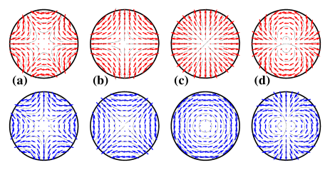
Figure 1: (color online) Electric (upper panels) and magnetic (lower panels) field $q$-filter geometries for different topological charges: (a) $q=-2$, (b) $q=-1$, (c) $q=1$, and (d) $q=+2$; in all cases $\beta=\pi/2$.

We are particularly interested in the negative $q$ geometries, which do not require to have a field source at $r=0$. For example, the $q=-1$ case corresponds to the standard quadrupole geometry of electron optics, while $q=-2$ corresponds to the hexapole one. Wien filters with such geometries have been already developed in the past for the purpose of correcting chromatic aberrations Rose (1970); Zach and Haider (1995). Moreover, inhomogeneous Wien filters including several multipolar terms have been also considered for the purpose of spin manipulation, with the added advantage of obtaining a stigmatic lensing behavior Scheinfein (1989). A possible design of the $q=-1$ filter with quadrupolar geometry is shown in Fig. 2.

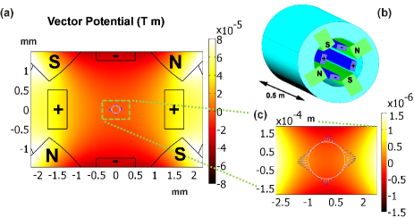
Figure 2: (color online) Electrodes and magnetic poles geometry of a $q$-filter with $q=-1$ (quadrupole), seen in cross-section (a) and in three-dimensional rendering (b). The filter length is set to 50 cm. In panel (a), the calculated vector potential $A_{z}$ (in false colors), which is also roughly proportional to the electric potential, and the projection on the $xy$ plane of the simulated electron ray trajectories for 100 keV energy are also shown (see SM for details about the simulations suppl ), for a ring-shaped input beam with radius $r=100$ $\mu$m (ray color grows darker for increasing $z$). In panel (c) a zoomed-in view of the central region. The magnetic field at $r$ needed to obtain the tuning condition $\delta=\pi$ is 3.5 mT, with a corresponding electric field of 575 kV/m. These are obtained with an electrode potential difference of $\approx 9$ kV and a magnetization of 135 A/mm. The fields need to be set to the design-values with a precision of 1 part in $10^{4}$.

In such non-uniform field geometry we cannot solve analytically the full Pauli’s equation. However, the beam propagation is already well described by classical dynamics and can be derived either analytically, using a power-expansion in $r$ Scheinfein (1989), or by numerical ray tracing. In the former case, we find that to first order the $q$-filter for $q\neq 0$ is already stigmatic, i.e., it preserves the beam circular symmetry. Only second-order corrections introduce aberration effects Scheinfein (1989). This behavior is confirmed by our numerical ray-tracing simulations (see SM for details suppl ), which show relatively weak higher-order aberrations (see Fig. 2). It should be noted that these simulations have been performed for realistic values of the electric and magnetic fields, as required to obtain a spin precession of half a turn across a propagation distance of 50 cm at a beam radius of 100 $\mu$m. These calculations are expected to reproduce very well the electron density behavior (and spin precession) as would be obtained from Pauli’s equation. However, Pauli’s equation predicts an additional purely quantum phenomenon, namely the geometric phase already discussed above. In a semi-classical approximation, the geometric phase will still be given by $\pm\alpha+\pi/2$, where $\alpha$ is however now position-dependent and given by Eq. (14). More specifically, neglecting the aberrations, each possible electron trajectory within a beam is straight and parallel to the $z$ axis. Therefore, the electrons travelling in a given trajectory will experience a constant magnetic field of modulus $B_{0}(r)$ and orientation $\alpha(\phi)$. The set of all electrons travelling at a given radius $r$ will then undergo a uniform spin precession by angle $\delta(r)$ and, if $\delta(r)=\pi$ (i.e., for a spin half-turn rotation), they will also acquire a space-variant geometric phase given by $\pm\alpha(\phi)+\pi/2=\pm q\phi\pm\beta+\pi/2$, with the $\pm$ sign determined by the input spin orientation. In other words, the outgoing wavefunction acquires a phase factor $\exp(i\ell\phi)$, with $\ell=\pm q$, corresponding to a vortex beam with OAM $\pm q\hbar$. In a quantum mechanical notation, spin-polarized input electrons with given initial OAM $\ell$ passing through a $q$-filter undergo the following transformations:

$$|\!\uparrow,\ell\rangle \rightarrow \cos(\delta/2)|\!\uparrow,\ell\rangle+ie^{i\beta}\sin(\delta/2)|\!\downarrow,\ell+q\rangle$$

$$|\!\downarrow,\ell\rangle \rightarrow \cos(\delta/2)|\!\downarrow,\ell\rangle+ie^{-i\beta}\sin(\delta/2)|\!\uparrow,\ell-q\rangle$$ (4)

where the ket indices now specify both the spin state (arrows) and the OAM eigenvalue.

Equations (Spin-to-orbital angular momentum conversion and spin-polarization filtering in electron beams) show that, in passing through the $q$-filter, a fraction $f=\sin^{2}(\delta/2)$ of the electrons in the beam will flip their spin and acquire an OAM $\pm q\hbar$, while the remaining fraction $1-f=\cos^{2}(\delta/2)$ will pass through the filter with no change. When $L=\Lambda_{1}/4$, then $\delta=\pi$ and all electrons are spin-flipped and acquire the corresponding OAM. In the specific case $q=1$, the spin angular momentum variation for the electrons undergoing the spin inversion is exactly balanced by the OAM variation, so that the total electron angular momentum remains unchanged in crossing the filter. This is the pure “spin-to-orbital conversion” STOC process mentioned in the introduction, and it occurs for $q=1$ because this geometry is rotationally invariant and therefore no angular momentum can be exchanged with the field sources in the filter. In the $q\neq 1$ case, the input spin still controls the sign of the OAM variation, but the total beam angular momentum is not conserved and some angular momentum is exchanged with the field sources. We note that this OAM variation can be also explained as the effect of the spin-related magnetic-dipole force acting on the electrons within the magnetic field gradients, as more fully discussed in the SM suppl .

The “tuning” condition $L=\Lambda_{1}/4$ or $\delta=\pi$ can be achieved in principle for a given radius $r$ by adjusting the strength of the magnetic and electric fields or the device length $L$. Since the precession angle $\delta$ is $r$-dependent, however, this tuning condition can be applied to the entire beam only if it is shaped as a ring, i.e. with all electron density peaked at a given radius $r$. Vortex beams with OAM $\ell\neq 0$ typically have a doughnut shape, so they approximate a ring fairly well. On the other hand a gaussian input beam (with $\ell=0$) cannot be fully transformed, as $\delta=0$ at $r=0$, where the beam has the maximum density. In such cases, only a fraction $f$ of the electrons would be converted.

So far we have assumed a spin-polarized input beam. However, high brightness (i.e., spatially coherent) spin-polarized electron beams, suitable for high-resolution TEM applications, are not so easily available. State-of-the-art spin-polarized sources may achieve a brightness of 10⁷ A cm^-2 sr^-1 and a polarization purity of up to 90% Yamamoto et al. (2011) (and the source decays with time due to laser-induced damage). It is interesting then to analyze the effect of the $q$-filter on a initially unpolarized electron beam, having arbitrary initial OAM $\ell$. Such input can be simply viewed as a statistical mixture in which 50% of the electrons are in the state $|\!\uparrow,\ell\rangle$ and 50% in the state $|\!\downarrow,\ell\rangle$. After passing through a tuned $q$-filter, the beam becomes a 50-50 mixture of states $|\!\downarrow,\ell+q\rangle$ and $|\!\uparrow,\ell-q\rangle$, for which spin and OAM are correlated (if the $q$-filter is not tuned, the fraction of converted electrons decreases to $f/2$ in each spinorbit state, and there will be a residual $1-f$ fraction of electrons in states $|\!\uparrow,\ell\rangle$ and $|\!\downarrow,\ell\rangle$). As we discuss now, this spin-OAM correlation can be exploited for making an effective electron beam spin-polarization filter. Such filter requires four basic elements in sequence (as shown in Fig. 2 of SM suppl ): (i) an OAM manipulation device, such as a fork hologram Verbeeck et al. (2010); McMorran et al. (2011), to set $\ell\neq 0$; (ii) a $q$-filter with $q=\ell$, generating a mixture of electrons in states $|\!\downarrow,2\ell\rangle$ and $|\!\uparrow,0\rangle$; (iii) a free propagation (or imaging) stage that allows these two states to develop different radial profiles by diffraction, because of their different OAM values; (iv) a circular aperture for finally separating the two states. In particular, in stage (iii) state $|\!\downarrow,2\ell\rangle$ will acquire a radial doughnut distribution, as in Laguerre-Gaussian modes with OAM $2\ell$, which vanishes close to the beam axis as $r^{2\ell}$, while state $|\!\uparrow,0\rangle$ will become approximately gaussian, with maximum intensity at the beam axis, as shown in Figs. 3a,b. Therefore, a suitable iris (Fig. 3c) will select preferentially the electrons in the fully polarized state $|\!\uparrow,0\rangle$. An optical OAM sorter exploiting a similar approach has been demonstrated recently Karimi et al. (2009).

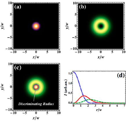
Figure 3: (color online) Electron beam profiles in the far field of the $q$-filter for the $\ell=0$ component (panel a) and the $\ell=2$ component (panel b), and a possible discriminating iris radius (panel c) $r=w$ to be used to separate them in order to make a spin-polarization filter. Panel (d) shows the intensity profiles of the same components ($\ell=0$ - blue dot-dashed line, $\ell=2$ - green dashed line) and of the possible residual $\ell=1$ component for an untuned $q$-filter (red solid line). $w$ is the gaussian beam waist radius in the far-field plane. A realistic value for the iris radius is of the order of several tens of microns (obtained by setting the aperture some distance after the focal plane of the second condensor)

A specific calculation for the case $|q|=|\ell|=1$ and an iris radius equal to the beam waist $w$ in the “far field” yields a transmission efficiency of our device of 55.5% (not including the losses arising in the OAM-manipulation device) and a polarization degree $(I_{\uparrow}-I_{\downarrow})/(I_{\uparrow}+I_{\downarrow})$, where $I_{\uparrow,\downarrow}$ are the two spin-polarized currents, of $\sim 97.5\%$. Higher degrees of polarization can be obtained at the expense of the efficiency by reducing the iris diameter or by employing higher $q$ values (or vice versa). It is worth noting that this apparatus works also with a partially tuned $q$-filter, as in this case the unmodified electron beam component is left in the initial OAM state $\ell=q$ and therefore is also cut-away by the iris. An untuned $q$-filter will however have an efficiency reduced by the factor $f=\sin^{2}(\delta/2)$. The aberrations introduced by the $q$-filter, even if left uncorrected, might also affect its efficiency but not its main working principle, as this is based on the vortex effect, which is protected by topological stability. Finally, the possible spin depolarization effect of fringe fields can be neglected if the length-to-gap ratio of the filter is large enough suppl ; Scheinfein (1989).

We note that the spin-filter application discussed above is a new counterexample of the old statement by Bohr that free electrons cannot be spin-polarized by exploiting magnetic fields, due to quantum uncertainty effects Darrigol (1984); Batelaan et al. (1997); Gallup et al. (2001). The reason why we can overcome Bohr’s arguments is essentially that we do not use the magnetic forces directly to obtain the separation, but take advantage of quantum diffraction itself, as also proposed recently in Ref. McGregor et al. (2011) (see SM for a fuller discussion suppl ).

In conclusion, we believe that the $q$-filter device described in this paper can be manufactured relatively simply, for applications in standard electron beam sources such as those used in TEMs or other kinds of electron microscopes. In combination with current field-effect unpolarized electron sources, such filter might provide a spin-polarized source with a brightness $\sim 10^{9}$ A cm^-2 sr^-1, about two orders of magnitude higher than the current state of the art. This result, if it will be proved practical enough, may open the way to a spin-sensitive atomic-scale TEM, e.g. suitable for investigating complex magnetic order in matter or for spintronic applications.

We acknowledge the support of the FET-Open Program within the 7^th Framework Programme of the European Commission under Grant No. 255914, Phorbitech.

Appendix: Supplementary Material

.1 Gaussian electron beam in homogeneous Wien filter

Let us consider an electron beam propagating in vacuum along the $z$-axis, subject to transverse and orthogonal electric and magnetic fields $\bm{E}$ and $\bm{B}$ lying in the $xy$ plane. In this Section, we assume the two fields to be spatially uniform, as in standard Wien filters, but we will release this assumption later on. If the magnetic field direction makes an angle $\alpha$ with the $x$-axis, we may write $\bm{E}=E_{0}(\sin{\alpha},-\cos{\alpha},0)$ and $\bm{B}=B_{0}(\cos{\alpha},\sin{\alpha},0)$. As scalar and vector potentials, we may then take $\Phi=-E_{0}(x\sin{\alpha}-y\cos{\alpha})$ and $\bm{A}=B_{0}\left(0,0,y\cos{\alpha}-x\sin{\alpha}\right)$, respectively. In the non-relativistic approximation and neglecting all Coulomb self-interaction effects (small charge density limit), the electron beam propagation is described by Pauli’s equation

$$i\hbar\partial_{t}\tilde{\psi}=\left[\frac{1}{2m}(-i\hbar\bm{\nabla}-e\bm{A})^{2}+e\Phi-\bm{B}\cdot\hat{\bm{\mu}}\right]\tilde{\psi}$$ (5)

where $\tilde{\psi}$ is the spinorial two-component wave-function of the electron beam, $e=-|e|$ and $m$ are the electron charge and mass, $\partial_{t}$ is the derivative with respect to the time variable $t$, $\hat{\bm{\mu}}=-\frac{1}{2}g\mu_{B}\hat{\bm{\sigma}}$ is the electron magnetic moment, with $\mu_{B}=\hbar|e|/2m$ the Bohr’s magneton, $g\simeq 2$ the electron $g$-factor, and $\hat{\bm{\sigma}}=(\hat{\sigma}_{x},\hat{\sigma}_{y},\hat{\sigma}_{z})$ the Pauli matrix vector.

We seek a monochromatic paraxial-wave solution with average linear momentum $p_{c}$ and average energy $E_{c}=p_{c}^{2}/2m$ in the form $\tilde{\psi}(x,y,z,t)=\exp[i(p_{c}z-E_{c}t)/\hbar]\tilde{u}(x,y,z)$, where $\tilde{u}(x,y,z)$ is taken to be a slow-varying envelope spinor field. Inserting this ansatz in Eq. (5) and neglecting small terms in the $z$ derivatives of $\tilde{u}$, we obtain the paraxial Pauli equation

$$\partial_{z}\tilde{u}=\frac{i}{2k_{c}}\left(\nabla^{2}_{\perp}-\frac{e^{2}}{\hbar^{2}}A^{2}+\frac{2m}{\hbar^{2}}\bm{B}\cdot\hat{\bm{\mu}}\right)\tilde{u}$$ (6)

where $\nabla^{2}_{\perp}=\partial_{x}^{2}+\partial_{y}^{2}$ is the Laplacian in the beam transverse plane and $k_{c}=p_{c}/\hbar$ is the De Broglie wavevector along the beam axis. In deriving Eq. (6) we set $E_{0}=p_{c}B_{0}/m$, so as to cancel out the average Lorentz force on the beam.

Equation (6) determines the evolution of the spinor field $\tilde{u}$ along the axis $z$. This equation can be solved analytically for the case of a gaussian input beam, as given by $\tilde{u}(r,\phi,0)=\tilde{a}\exp[-r^{2}/w_{0}^{2}]$ for $z=0$, where $w_{0}$ is the beam waist and $\tilde{a}=(a_{1},a_{2})$ the input spinor, corresponding to an arbitrary spin superposition $|\psi\rangle=a_{1}|\uparrow\rangle+a_{2}|\downarrow\rangle$. A straightforward calculation shows that the solution is given by

$$\tilde{u}(r,\phi,z)=G(r,\phi,z)\hat{M}(z)\tilde{a}$$ (7)

where $\hat{M}(z)$ is the matrix

$$\hat{M}(z)=\begin{pmatrix}\cos\frac{2\pi z}{\Lambda_{1}}&ie^{-i\alpha}\sin\frac{2\pi z}{\Lambda_{1}}\\ ie^{i\alpha}\sin\frac{2\pi z}{\Lambda_{1}}&\cos\frac{2\pi z}{\Lambda_{1}}\end{pmatrix}$$ (8)

where $\Lambda_{1}=(2\pi\hbar^{2}k_{c})/(mg\mu_{B}B_{0})$ and the scalar gaussian factor $G(r,\phi,z)$ is given by

$$G(r,\phi,z)=g_{0}(z)e^{ik_{c}r^{2}\left(\frac{\cos^{2}(\alpha-\phi)}{2q_{1}(z)}+\frac{\sin^{2}(\alpha-\phi)}{2q_{2}(z)}\right)}$$ (9)

with

$$g_{0}(z) = \frac{\sqrt{\pi}\,z_{R}\,e^{-\frac{i}{2}\arctan{\left(\frac{z}{z_{R}}\right)}}\,\,e^{-\frac{i}{2}\arctan\left(\frac{\Lambda_{2}}{\pi z_{R}}\tan\frac{\pi z}{\Lambda_{2}}\right)}}{(z_{R}^{2}+z^{2})^{\frac{1}{4}}\left(\pi^{2}z_{R}^{2}\cos^{2}\frac{\pi z}{\Lambda_{2}}+\Lambda_{2}^{2}\sin^{2}\frac{\pi z}{\Lambda_{2}}\right)^{\frac{1}{4}}},$$ (10)

$$q_{1}(z) = z-iz_{R},$$ (11)

$$q_{2}(z) = \frac{\Lambda_{2}}{\pi}\left(\frac{\Lambda_{2}\sin(\frac{\pi z}{\Lambda_{2}})-i\pi z_{R}\cos(\frac{\pi z}{\Lambda_{2}})}{\Lambda_{2}\cos(\frac{\pi z}{\Lambda_{2}})+i\pi z_{R}\sin(\frac{\pi z}{\Lambda_{2}})}\right),$$ (12)

where $z_{R}=\frac{1}{2}k_{c}w_{0}^{2}$ and $\Lambda_{2}=\frac{\pi\hbar k_{c}}{eB_{0}}=g\Lambda_{1}/4\simeq\Lambda_{1}/2$.

The matrix $\hat{M}(z)$ given in Eq. (8) corresponds to Eq. 2 in the main paper and describes the magnetic-field-induced Larmor spin precession during propagation and the associated geometric phases discussed in the main paper. The precession length $\Lambda_{1}$ corresponds to two full spin rotations.

In addition to the spin dynamics, from Eq. (12), we find that the wavefront complex curvature radius $q_{2}(z)$ in the direction perpendicular to the magnetic field $\bm{B}$ changes periodically with spatial period $\Lambda_{2}$. These oscillations correspond to the well known astigmatic lensing effect of the Wien filter.

.2 Space-variant Wien filter and ray-tracing simulations

In this Section, we consider “$q$-filter” field geometries with cylindrical symmetry, described by the following expression for the magnetic field (with the vector given in cartesian components):

$$\bm{B}(r,\phi,z)=B_{0}(r)(\cos{\alpha(\phi)},\sin{\alpha(\phi)},0)$$ (13)

where the angle $\alpha$ is now the following function of the azimuthal angle:

$$\alpha(r,\phi,z)=q\phi+\beta$$ (14)

where $q$ is an integer and $\beta$ a constant. As discussed in the main paper, such a field pattern must have a singularity of topological charge $q$ at the beam axis $r=0$. In particular, by imposing the vanishing of the field divergence, we find that the radial factor $B_{0}(r)\sim r^{-q}$, i.e., the field vanishes on the axis for negative values of $q$, while it diverges for positive values of $q$. In the latter case, there must be a field source on the axis. The electric field will be taken to have an identical pattern, except for a local $\pi/2$ rotation, so as to balance everywhere the Lorentz force. We are particularly interested in the negative $q$ geometries, which do not require to have a field source at the beam axis. For example, the $q=-1$ case corresponds to the standard quadrupole geometry, while $q=-2$ corresponds to an hexapole one.

The electron propagation problem in such non-uniform field can only be solved approximately or numerically. A second-order geometrical optics solution is reported in Ref. scheinfein89, which includes also a detailed analysis of spin precession but without considering the geometric phase effect (as well as the magnetic dipole forces). This analysis shows that, to first order, a balanced Wien filter having quadrupole or hexapole geometry but vanishing dipole term (as in our $q$-filter) is already stigmatic, i.e. it preserves the cylindrical symmetry without need for further corrections. The only beam lensing or distortion effects enter as higher-order aberrations (i.e., the $G$ term in Eq. (31) of Ref. scheinfein89).

To further analyze the behavior of our $q$-filter, we have performed ray-tracing simulations of the electron propagation for a quadrupole geometry ($q=-1$). The magnetic and electric fields have been calculated using COMSOL finite-elements simulation (www.comsol.com). The ray-tracing routines therein contained have been used to assess the shape of the beam at the exit of the filter starting from an input beam having 100 keV of enery that is shaped as a ring, with a radius $r$ of 100 $\mu$m. The magnetic field at $r$ needed to obtain the tuning condition $\delta=\pi$ is 3.5 mT, with a corresponding electric field of 575 kV/m. These are obtained in our geometry with an electrode potential difference of $\approx 9$ kV and a magnetization of 135 A/mm. The fields need to be set to the design-values with a precision of 1 part in $10^{4}$. The electron velocity to be used as initial conditions in the simulations must be obtained from a model of the fringe fields. For the simplest description of the input fringe fields, i.e. the so-called sharp cut-off fringing field (SCOFF) model, the transverse velocity components remain constant and nil, i.e. $v_{x}=v_{y}=0$, while the $z$-component $v_{z}(x,y)$ “just inside” the filter is given by the following expression:

$$v_{z}(x,y)=v_{0}-\frac{e\Phi(x,y)}{mv_{0}}=v_{0}-\frac{eA_{z}(x,y)}{m}$$ (15)

where $v_{0}$ is the velocity outside the filter. This condition is derived from the conservation of energy and also ensures the conservation of the canonical momentum of the electrons entering the Wien filter and hence the conservation of their wavefront orientation.

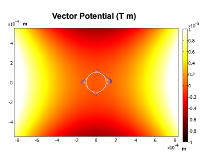
Figure 4: Projection on the $xy$ plane of the simulated trajectories of the electrons starting from a circle of radius $r=100$ $\mu$m. The trajectories are shown with a color growing darker as $z$ is increased.

The results of ray-tracing simulations are reported in Fig. 2 of the main paper and in Fig. 4 of the present manuscript, which show how a circle of electron positions representative of the input beam becomes deformed during the propagation into a quadrupole-lobed shape, due to second- or higher-order aberrations. For optimizing the performances of our proposed device, in particular in the spin-polarization filter application, these aberrations should probably be compensated by additional electron optics (e.g., octupole electrostatic lenses). Nevertheless, even for no aberration compensation, the vortex effect giving rise to the radial separation of the two spin components discussed in the spin-polarization application is expected to be preserved, owing to its topological stability.

.3 Magnetic dipole forces and angular momentum

We now evaluate the effects of the force associated with the magnetic dipole of the electrons in the magnetic field gradient of the Wien filter. This is the force used in Stern-Gerlach experiments and the only spin-dependent force acting on the electrons, so it is important to assess its effects in detail. At any given point inside the filter, assuming that the magnetic dipole of the electron is $\bm{\mu}=-g\mu_{B}\bm{S}$, where $\bm{S}$ is the corresponding spin vector, the associated magnetic force is

$$\bm{F}=\nabla(\bm{\mu}\cdot\bm{B})$$ (16)

where the gradient must be taken while keeping $\bm{\mu}$ constant, i.e. acting only on the magnetic field coordinates. For our classical estimate, the magnetic dipole evolution can be described by the precession equation

$$\frac{d\bm{\mu}}{dt}=\frac{g|e|}{2m}\bm{B}\times\bm{\mu}$$ (17)

Assuming a starting magnetic moment parallel to the $z$ axis, the magnetic dipole will rotate around the local magnetic field direction. In the approximation in which aberrations are neglected, each electron travels along a parallel ray with constant transverse coordinates, and hence sees a uniform magnetic field, given by Eq. (13). Therefore, the magnetic dipole at any given point inside the filter will be given by the following expression:

$$\bm{\mu}(r,\phi,z) = \mu_{B}[-\sin\delta(r,z)\sin{\alpha(\phi)},\sin\delta(r,z)\cos{\alpha(\phi)},$$ (18)

$$\cos\delta(r,z)]$$

where $\delta(r,z)$ is the total spin precession angle at $z$, for a trajectory at radius $r$. Taking the scalar product between $\bm{\mu}$ and $\bm{B}$ and then the gradient with respect to the coordinates of $\bm{B}$ only, we find that the magnetic dipole force is only directed along the azimuthal direction and given by

$$\bm{F}=\hat{\bm{\phi}}q\frac{\mu_{B}B_{0}(r)}{r}\sin\delta(r,z)$$ (19)

where $\hat{\bm{\phi}}$ denotes the unit vector along the azimuthal direction and we have used Eq. (14) for taking the $\phi$ derivative.

Equation (19) can be used for two purposes. First, we can verify that the ray deflection inside the Wien filter due to this force is negligible. Indeed, integrating the force in the time $T$ needed for a full $\pi$ rotation of the spin (or spin flip), we obtain the overall momentum change

$$\Delta p_{\phi} = \int_{0}^{T}F_{\phi}(t)dt=\int_{0}^{\pi}F_{\phi}(\delta)\left(\frac{d\delta}{dt}\right)^{-1}d\delta$$ (20)

$$=\frac{2m}{g|e|B_{0}}\int_{0}^{\pi}F_{\phi}(\delta)d\delta=\frac{2q\hbar}{gr}$$

We can see from this equation that the momentum variation is of the same order as the quantum uncertainty in momentum of the electron wavefunction, taking into account that the position uncertainty is of the same order of the beam size $r$ (as it is also expected based on Bohr impossibility theorem, as discussed further below). This momentum change produces negligible effects in the electron propagation across the filter, although it instead becomes relevant in the far field. Indeed, it is precisely this force that produces the orbital angular momentum change at the basis of our spin selection. Indeed, we will now show that the torque associated with the magnetic dipole force is that responsible for the OAM change of the electrons. The $z$-component torque of this force is given by

$$M_{z} = (\bm{r}\times\bm{F})_{z}=q\mu_{B}B_{0}(r)\sin\delta=q(\bm{\mu}\times\bm{B})_{z}$$ (21)

$$=-q\frac{dS_{z}}{dt}$$

where $S_{z}$ is the $z$ component of the electron spin angular momentum $\bm{S}$. Since this torque acts on the OAM of the electrons $L_{z}$, we find the following angular momentum coupling law:

$$\frac{dL_{z}}{dt}=-q\frac{dS_{z}}{dt}$$ (22)

Once integrated for the entire flight time, corresponding to a full spin flip, this coupling law returns the same result reported in the main paper for the OAM variation induced by the spin flip.

This correspondence proves that the effect, and the only effect, of the magnetic dipole force acting on the electrons is the change of OAM already considered by including the geometric phase shift in the wavefunction emerging from the filter. Therefore, the only significant effect of this force appears in the far field and is exactly the effect that we propose to utilize to separate electrons according to their spin.

.4 Fringe field effects

The actual fringe fields depend on the electrodes and magnetic poles geometry. It is however safe to assume that the fringe fields extend only for a longitudinal distance along the $z$ axis that is comparable to the transverse aperture of the Wien filter, and therefore much smaller than the filter length, in the large length-to-gap ratio limit. Moreover, the transverse components of the fringe fields can be taken to have exactly the same multipolar geometry as the fields inside the Wien, and hence will give rise to similar effects both in lensing and spin precession. Their overall effect is therefore only to change the effective length of the filter. However, in addition there will also be a longitudinal $z$ component that must be taken into account. In the lensing effect, only the $z$ component of the electric field plays a role, by ensuring the validity of the condition (15). The $z$ component of the magnetic fields does not affect the ray propagation, since it exerts a vanishing Lorentz force. However, the latter may affect the spin precession. If we assume that the input electrons have a spin parallel to the $z$ axis, then the $z$ component of the fringe magnetic field does nothing. However, the spin may be somewhat rotated away from the $z$ axis by the transverse fringe magnetic field, and in this case the longitudinal component will induce some non-uniform precession around the $z$ axis that may partly depolarize the beam. This effect will however be proportional to the time spent by the particles in the fringe field region, and hence will be negligible in the large length-to-gap ratio limit.

We may also consider the idealized limit of an extremely thin fringe field region in which the electric and magnetic fields vary rapidly from the vanishing values they have away from the Wien filter to the values they acquire well inside the filter, which then remain perfectly constant. This is the SCOFF limit mentioned above. In particular, in the SCOFF limit the vector potential $\bm{A}$ must go from zero to the value $\bm{A}=[0,0,A_{z}(x,y)]$ describing the multipolar magnetic field inside the filter. This rapid transition does not give rise to any magnetic field, because it is curl-free. Therefore, the SCOFF limit has vanishing magnetic fringe fields and therefore absolutely no effect on the spin, nor on the lensing behavior of the filter. On the other hand, in the SCOFF limit the electric potential must go from zero to the nonzero value $\Phi(x,y)$ describing the multipolar electric field inside the filter. This in turn implies the presence of a very strong longitudinal electric fringe field that is responsible for the change of velocity given by Eq. (15). We stress that this idealized SCOFF description of the fringe fields needs not being realistic, but it is sufficient to identify the ineliminable effects that the fringe field impose to the electrons, and therefore the possible fundamental limitations that may arise from them.

.5 Layout of a spin-polarized TEM microscope

We report in Fig. 5 the sketch of a possible TEM microscope incorporating the proposed spin-polarization filter based on the $q$-filter. Such a device could be used to perform spin-sensitive TEM microscopy on magnetic materials or spintronic devices.

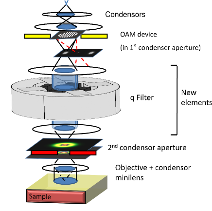
Figure 5: Sketch of a possible TEM microscope incorporating the proposed spin-polarization filter based on the $q$-filter.

It includes the four stages discussed in the main paper, i.e. (i) the fork hologram to set the initial OAM, (ii) the $q$-filter to couple OAM to spin, (iii) an imaging stage to go in the Fourier plane, (iv) an aperture to select a single spinorbit component, as well as the additional electron optics needed for imaging and collimating the beam. The input aperture of the system is defined by the fork hologram mask and has a typical radius of few microns Verbeeck et al. (2010). The output iris needed to select a single spin polarization can be set to a radius of few tens of microns, by carefully selecting the aperture plane position with respect to the focal plane. It will be presumably convenient to work slightly off focus to obtain larger beam waists without the need to introduce additional magnifying optics.

We note here in passing that in the new generation of TEM microscopes with aberration-corrected probe a larger number of lenses are available for beam control, and in particular a pair of hexapoles. It could be worth then exploring the possibility of using directly these lenses as an effective $q$-filter, without introducing additional optical elements. In this configuration, the magnetic hexapoles with opposite sign could be used to produce the polarization, while also compensating the introduced aberration. However stability issues might arise for large fields and the effect of fringing fields on the spin may also not be negligible, in this case, as the length-to-gap ratio would not be very large. Therefore, further analysis and simulations will be necessary in order to assess this possibility.

.6 The role of electron diffraction

In our treatment we fully included the diffraction effects only in the free propagation (through a lensing system) taking place after the $q$-filter device. Indeed, this stage is where the correlation between OAM and radial profile develops and is then exploited for separating the different spin components. This free propagation, ending in the far-field and giving rise to the beam profiles shown in Fig. 3 of the main paper, has been evaluated using a fully quantum mechanical treatment. The diffraction effects are obviously important in the propagation from near to far field, and in particular in determining the presence or absence of destructive interference effects at the vortex position that are essential in our proposed scheme.

One may wonder if we can legitimately ignore the diffraction effects in the other stages of our proposed setup. For the propagation through the $q$-filter, we could assess directly the role of diffraction in the case of homogeneous field, for which we have both the exact solution of Pauli’s equation (including diffraction) and the classical trajectory solutions. We find that diffraction is only relevant if we look at the electron beam very close to a focal point, where its width becomes of the order of few nanometers. Away from the focus, the ensemble of classical trajectories reproduces perfectly well the quantum beam evolution. This result is not surprising, as in the $q$-filter all length scales are 8–9 orders of magnitude larger than the electron wavelength $\lambda=2\pi/k_{c}$, which is of few picometers for energies of the order of 100 keV (typical of electron microscopes). Therefore, we may safely assume that diffraction can be ignored also in inhomogeneous $q$-filter geometries, as long as no focusing occurs inside the filter. Our classical ray-tracing simulations confirm that we avoid a focusing inside the $q$-filter. It should be also noted that in designing and analyzing electron-optics elements as those commonly used in electron microscopy, it is quite standard to ignore quantum effects and use classical ray tracing or geometrical optics.

The input and output apertures, being again about 7 orders of magnitude larger than the electron wavelength, will also give negligible diffraction effects (only some radial fringes extremely close to the aperture edges are expected, which should not affect the proper working of the proposed setup).

.7 Violation of Bohr’s “theorem”

As reported in Ref. Darrigol (1984), few years after the discovery of electron spin, several experiments were proposed (and sometimes attempted) aimed at separating electrons according to their spin, mainly by exploiting inhomogeneous magnetic fields acting on the magnetic dipole associated with it (similar to the Stern-Gerlach experiment). In 1929, Niels Bohr demonstrated a sort of “impossibility theorem” Darrigol (1984), stating that no Stern-Gerlach-like experiment (including Knauer’s proposal, in which an electric field was used to balance the Lorentz force) could be used to separate electrons according to their spin by more than a small fraction of the beam transverse extension. This was related to the uncertainty principle and to the unavoidable orthogonal magnetic field accompanying the required magnetic field gradient. A simple explanation of this result is that the spin magnetic moment vanishes in the classical limit $\hbar\rightarrow 0$, so all attempts at separating particles according to the magnetic-moment force occurring in a magnetic field gradient give rise to a vanishing separation in the classical limit, and hence a separation that is comparable to quantum uncertainty. Actually, this statement has been later proved not to be strictly valid (see, e.g., Refs. Batelaan et al. (1997); Gallup et al. (2001)), although it remains extremely hard to overcome in practice.

Our approach is however fundamentally different from past attempts. Indeed, we exploit the quantum nature itself of the electrons to operate the spin separation (as such, our proposal bears some similarities with a very recently proposed scheme for spin-polarization in which electron diffraction is also exploited McGregor et al. (2011)). As we have seen, the magnetic dipole force in our device acts only in the azimuthal direction, which is not the direction along which we separate the electrons. The torque associated with this force imparts the OAM variation corresponding to the azimuthal geometric phase. However, at the exit of our Wien filter the electrons show no significant spatial separation according to the spin. It is then the subsequent free propagation and diffraction that acts to separate the electrons along the radial direction, which is not the direction of the main field gradient. In particular, an efficient radial separation is ensured by the presence of a vortex at the beam axis for one spin component and not for the other. In other words, we use the quantum wavy nature of the electrons to separate them according to the spin, and hence our method is not subject to Bohr’s impossibility theorem. As a further argument, even in the classical Stern-Gerlach approach Bohr’s theorem does not forbid the creation of spin-polarized components at the edges of the beam, so that by suitable aperturing it should be possible to generate spin-polarized beams, although with very low efficiency. Our method is also based on selecting only an edge of the beam, although this is done in the radial direction and the efficiency is strongly improved by the vortex-related destructive interference effects. Finally, we note that in our geometry the unavoidable orthogonal magnetic field associated with the azimuthal field gradient generating the dipole forces, which is the main source of problems in the Stern-Gerlach approach to spin-polarized electron separation, is already taken into account and corresponds to the radial magnetic field of the quadrupole or hexapole configuration. So its effect has been already fully considered in our treatment.

References

- Uchida and Tonomura (2010) M. Uchida and A. Tonomura, Nature 464, 737 (2010).
- Verbeeck et al. (2010) J. Verbeeck, H. Tian, and P. Schattschneider, Nature 467, 301 (2010).
- McMorran et al. (2011) B. J. McMorran et al., Science 331, 192 (2011).
- Bliokh et al. (2007) K. Y. Bliokh, Y. P. Bliokh, S. Savel’ev, and F. Nori, Phys. Rev. Lett. 99, 190404 (2007).
- Franke-Arnold et al. (2008) S. Franke-Arnold, L. Allen, and M. J. Padgett, Laser Photonics Rev. 2, 299 (2008).
- Marrucci et al. (2006) L. Marrucci et al., Phys. Rev. Lett. 96, 163905 (2006).
- Marrucci et al. (2011) L. Marrucci et al., J. Opt. 13, 064001 (2011).
- Tioukine and Aulenbacher (2006) V. Tioukine and K. Aulenbacher, Nucl. Instr. Meth. A 568, 537 (2006).
- Grames et al. (2011) J. Grames et al., Proc. of 2011 particle accelerator conf., New York, NY, USA (2011).
- (10) See the supplemental material in the Appendix.
- Shapere and Wilczek (1988) A. Shapere and F. Wilczek, eds., Geometric Phases in Physics (World Scientific, Singapore, 1988).
- Rose (1970) H. Rose, Optik 32, 144 (1970).
- Zach and Haider (1995) J. Zach and M. Haider, Nucl. Instr. and Meth. A 363, 316 (1995).
- Scheinfein (1989) M. R. Scheinfein, Optik 82, 99 (1989).
- Yamamoto et al. (2011) N. Yamamoto et al., J. Phys.: Conf. Ser. 298, 012017 (2011).
- Karimi et al. (2009) E. Karimi et al., Appl. Phys. Lett. 94, 231124 (2009).
- Darrigol (1984) O. Darrigol, Hist. Stud. Phys. Sci. 15, 39 (1984).
- Batelaan et al. (1997) H. Batelaan et al., Phys. Rev. Lett. 79, 4517 (1997).
- Gallup et al. (2001) G. A. Gallup et al., Phys. Rev. Lett. 86, 4508 (2001).
- McGregor et al. (2011) S. McGregor et al., New J. Phys. 13, 065018 (2011).