Abstract

The dynamics of a general two qubits system in noninetrial frame is investigated analytically, where it is assumed that both of its subsystems are differently accelerated. Two classes of initial travelling states are considered:self transposed and a generic pure states. The entanglement contained in all possible generated entangled channels between the qubits and their Anti-qubits is quantified. The usefulness of the travelling channels as quantum channels to perform quantum teleportation is investigated. For the self transposed classes, we show that the generalized Werner state is the most robust class. We show that starting from a class of pure state, one can generate entangled channels more robust than self transposed classes.

1 Introduction

Due to its importance in quantum information and computation fields, entanglement has attracted extensive attentions [1]. The dynamics of entanglement in the real and practical setting cases is one of the most promising technique to develop the efficiency of communication and computations [2]. Recently, the dynamics of entanglement is extended to the relativistic world [3]. In this direction, efforts have been done to investigate the dynamics of entanglement between two modes of Dirac modes in noninertial frames. It has been shown that, the degree of entanglement between entangled observers is degraded and consequently the accelerated observer can’t obtain information about his space time [3]. The dynamics of entanglement in non-inertial frames for two qubits system initially prepared in maximum entangled state is investigated in [3], where the entanglement is degraded by the Unruh effect [9] and its lower limit is enough for quantum teleportation. The sudden death of entanglement and the dynamics of mutual information are investigated by Landulfo and Matsas [5] in non-inertial frames. The dynamics of the classical and non-classical correlations of travelling pseudo-pure are investigated by H. Mehri-Dehnavi et. al. [6]. The entanglement dynamics of initial tripartite class of GHZ state is investigated in [7]. Montero et. al [8], have introduced tripartite W -state as initial travelling states, where they showed that the entanglement vanishes completely in the infinite acceleration limit.

In this contribution, we investigate the dynamics of a general two qubits state of Dirac field in non-inertial frame. First, an analytical solution is introduced for a general two qubits system. Particularly, we investigate two classes extensively: the self transposed class and a class of a generic pure state. Second, the degree of entanglement is quantified for all possible generated entangled channels between the qubits and their Anti-qubits. Third, the usefulness of the travelling accelerated classes is investigated by means of the fidelity and the possibility of using them as quantum channels to perform the quantum teleportation is discussed.

The outline of the article is as follows. In Sec.2, we introduce an analytical solution of the suggested model, where it is assumed that both qubits are accelerated. Sec.3 is devoted to investigate the dynamics of the self transposed classes and a class of a generic pure state. The entanglement of the generated entangled channels is quantified in Sec.4. The classification of usefulness travelling accelerated qubits are investigated in Sec.5. Finally, we summarize our results in Sec.6.

2 The suggested model and its evolution

Assume that a source supplies two partners Alice and Rob with a general two qubits state which is characterised by $15$ parameters. The general form of this system can be written as,

$$\rho_{AR}=\frac{1}{4}(1+\mathord{\buildrel\lower 3.0pt\hbox{$\scriptscriptstyle\rightarrow$}\over{s}}\cdot{\sigma^{\raisebox{2.0pt}[0.0pt]{$\scriptstyle\downarrow$}}}_{x}+\mathord{\buildrel\lower 3.0pt\hbox{$\scriptscriptstyle\rightarrow$}\over{t}}\cdot{\tau^{\raisebox{2.0pt}[0.0pt]{$\scriptstyle\downarrow$}}}+\mathord{\buildrel\lower 3.0pt\hbox{$\scriptscriptstyle\rightarrow$}\over{\sigma}}\cdot\mathord{\begin{picture}(12.0,12.0)(-1.0,0.0)\put(-3.0,12.0){\makebox(0.0,0.0)[t]{$\scriptscriptstyle\downarrow$}} \put(-3.0,13.0){\makebox(0.0,0.0)[l]{$\scriptscriptstyle\longrightarrow$}} \put(5.0,0.0){\makebox(0.0,0.0)[b]{$C$}} \end{picture}}\cdot{\tau^{\raisebox{2.0pt}[0.0pt]{$\scriptstyle\downarrow$}}}),$$ (1)

where $\mathord{\buildrel\lower 3.0pt\hbox{$\scriptscriptstyle\rightarrow$}\over{\sigma}}_{i}=(\sigma_{x},\sigma_{y},\sigma_{z}),\mathord{\buildrel\lower 3.0pt\hbox{$\scriptscriptstyle\rightarrow$}\over{\tau}}_{i}=(\tau_{x},\tau_{y},\tau_{z})$ are the Pauli matrices for Alice and Rob’s qubit respectively, $\mathord{\buildrel\lower 3.0pt\hbox{$\scriptscriptstyle\rightarrow$}\over{s}}=(s_{x},s_{y},s_{z})$ with $s_{i}=tr\{\rho_{AB}\sigma_{i}\}$ and $\mathord{\buildrel\lower 3.0pt\hbox{$\scriptscriptstyle\rightarrow$}\over{t}}=(t_{x},t_{y},t_{z}),$ $t_{i}=tr\{\rho_{AB}\tau_{i}\}$ are Bloch vectors for both qubits respectively. The dyadic $\mathord{\begin{picture}(12.0,12.0)(-1.0,0.0)\put(-3.0,12.0){\makebox(0.0,0.0)[t]{$\scriptscriptstyle\downarrow$}} \put(-3.0,13.0){\makebox(0.0,0.0)[l]{$\scriptscriptstyle\longrightarrow$}} \put(5.0,0.0){\makebox(0.0,0.0)[b]{$C$}} \end{picture}}$is a $3\times 3$ matrix with elements are defined by $c_{ij}=tr\{\rho_{AB}\sigma_{i}\tau_{i}\}$. For example, $c_{xx}=tr\{\rho_{AB}\sigma_{x}\tau_{x}\},c_{xy}=tr\{\rho_{AB}\sigma_{x}\tau_{y}\},c_{xz}=tr\{\rho_{AB}\sigma_{x}\tau_{x}\}$ and so on. The density operator (1) $\rho_{AR}$ can be written as $4\times 4$ matrix its elements are given by,

$$\varrho_{11} = \frac{1}{4}(1+s_{z}+t_{z}+c_{zz}),\quad\quad\varrho_{12}=\frac{1}{4}(t_{x}-it_{y}+c_{zx}+ic_{zy})$$

$$\varrho_{13} = \frac{1}{4}(s_{x}-is_{y}+c_{xz}-ic_{yz}),\quad\ \varrho_{14}=\frac{1}{4}(c_{xx}-ic_{xy}-ic_{yx}-c_{yy}),$$

$$\varrho_{21} = \frac{1}{4}(t_{x}-it_{y}+c_{zx}+ic_{zy}),\quad\varrho_{22}=\frac{1}{4}(1+s_{z}+t_{z}-c_{zz}),$$

$$\varrho_{23} = \frac{1}{4}(c_{xx}+ic_{xy}-ic_{yx}+c_{yy})\quad\varrho_{24}=\frac{1}{4}(s_{x}-is_{y}-c_{xz}+ic_{yz})$$

$$\varrho_{31} = \frac{1}{4}(s_{x}+is_{y}+c_{xz}+ic_{yz}),\quad\varrho_{32}=\frac{1}{4}(c_{xx}-ic_{xy}+ic_{yx}+c_{yy}).$$

$$\varrho_{33} = \frac{1}{4}(1-s_{z}+t_{z}-c_{zz}),\quad\quad\varrho_{34}=\frac{1}{4}(t_{x}-it_{y}-c_{zx}+ic_{zy}),$$

$$\varrho_{41} = \frac{1}{4}(c_{xx}-ic_{xy}+ic_{yx}-c_{yy}),\quad\varrho_{42}=\frac{1}{4}(s_{x}+is_{y}-c_{xz}-ic_{yz}),\quad$$

$$\varrho_{43} = =\frac{1}{4}(t_{x}+it_{y}-c_{zx}-ic_{zy}),\quad\varrho_{44}=\frac{1}{4}(1-s_{z}-t_{z}+c_{zz}).$$ (2)

The density operator (1) represents a quantum channel between Alice and Rob in the inertial frame. To study the dynamics of the travelling channel (1) in non-inertial frames we use what is called the Unruh modes [9] which are defined as,

$$\bigl{|}0\bigr{\rangle}_{i} = \mathcal{C}_{i}\bigl{|}0\bigr{\rangle}_{I}\bigl{|}0\bigr{\rangle}_{II}+\mathcal{S}_{i}\bigl{|}1\bigr{\rangle}_{I}\bigl{|}1\bigr{\rangle}_{II},$$

$$\bigl{|}1\bigr{\rangle}_{i} = \bigl{|}1\bigr{\rangle}_{I}\bigl{|}1\bigr{\rangle}_{II},$$ (3)

where $\mathcal{C}_{i}=\cos r_{i},\mathcal{S}_{i}=sinr_{i},$ with $tanr_{i}=e^{-2\pi\omega_{i}\frac{c}{a_{i}}}$, $a_{i}$ is the acceleration, $\omega_{i}$ is the frequency of the travelling qubits, $c$ is the speed of light and $i=A,R$. In this investigation, it is assumed that Alice and Rob are observers and can lie in either region of Rindler space time. Therefore, a uniformly accelerated observer lying in one wedge of space time is causally disconnected from the other. This leads to four different situations: (i) the channel between Alice and Rob $\rho_{\tilde{A}_{I}\tilde{R}_{I}}$ is in the region $I$, which requires to trace out the states in mode $II$.(ii) The channel between Anti-Alice and Anti-Rob $\rho_{\tilde{A}_{II}\tilde{R}_{II}}$ is in the region $II$ which requires to trace out the states in mode $I$. (iii) The channel between Alice and Anti-Rob $\rho_{\tilde{A}_{I}\tilde{R}_{II}}$, which is obtained by tracing out Anti-Alice mode in the region $II$ and the mode of Rob in mode $I$. (v) The channel between Rob and Anti-Alice, $\rho_{\tilde{A}_{II}\tilde{R}_{I}}$ which is obtained by tracing out Alice’s mode in the region $I$ and Rob’s mode in the region $II$.

By using Eq.(1), (2) and tracing out the inaccessible modes in the region $II$, the state of Alice-Rob in the region $I$ is described by,

$$\rho_{\tilde{A}_{I}\tilde{R}_{I}}=\left(\begin{array}[]{cccc}\varrho_{11}\mathcal{C}_{1}^{2}\mathcal{C}_{2}^{2}&\varrho_{12}\mathcal{C}_{1}^{2}\mathcal{C}_{2}&\varrho_{13}\mathcal{C}_{1}\mathcal{C}_{2}^{2}&\varrho_{14}\mathcal{C}_{1}\mathcal{C}_{2}\\ \\ \varrho_{21}\mathcal{C}_{1}^{2}\mathcal{C}_{2}&\mathcal{C}_{1}^{2}(\varrho_{22}+\varrho_{11}\mathcal{S}_{2}^{2})&\varrho_{23}\mathcal{C}_{1}\mathcal{C}_{2}&\varrho_{24}\mathcal{C}_{1}\\ \\ \varrho_{31}\mathcal{C}_{1}\mathcal{C}_{2}&\varrho_{32}\mathcal{C}_{1}\mathcal{C}_{2}&(\varrho_{33}+\varrho_{11}\mathcal{S}_{1}^{2})\mathcal{C}_{2}^{2}&(\varrho_{34}+\varrho_{12}\mathcal{S}_{1}^{2})\mathcal{C}_{2}\\ \\ \varrho_{41}\mathcal{C}_{1}\mathcal{C}_{2}&(\varrho_{42}+\varrho_{31}\mathcal{S}_{2}^{2})\mathcal{C}_{1}&(\varrho_{43}+\varrho_{21}\mathcal{S}_{1}^{2})\mathcal{C}_{2}&\varrho_{44}+\varrho_{33}\mathcal{S}_{2}^{2}+(\varrho_{22}+\varrho_{11}\mathcal{S}_{2}^{2})\\ \end{array}\right).$$ (4)

Similarly, if we trace out the inaccessible modes in the region $I$, one gets the density operator of Alice-Rob in the region$II$ as,

$$\rho_{\tilde{A}_{II}\tilde{R}_{II}}=\left(\begin{array}[]{cccc}\varrho^{(II)}_{11}&(\varrho_{43}+\varrho_{21}\mathcal{C}_{1}^{2})\mathcal{S}_{2}&(\varrho_{42}+\varrho_{31}\mathcal{C}_{2}^{2})\mathcal{S}_{1}&\varrho_{41}\mathcal{S}_{1}\mathcal{S}_{2}\\ \\ (\varrho_{34}+\mathcal{C}_{1}^{2}\varrho_{12})\mathcal{S}_{2}^{2}&(\varrho_{33}+\varrho_{11}\mathcal{C}_{1}^{2})\mathcal{S}_{2}^{2}&\varrho_{32}\mathcal{S}_{1}\mathcal{S}_{2}&\varrho_{31}\mathcal{S}_{1}\mathcal{S}_{2}^{2}\\ \\ (\varrho_{24}+\varrho_{13}\mathcal{C}_{2}^{2})\mathcal{S}_{2}^{2}&\varrho_{23}\mathcal{S}_{1}\mathcal{S}_{2}&(\varrho_{22}+\varrho_{11}\mathcal{C}_{2}^{2})\mathcal{S}_{1}^{2}&\varrho_{21}\mathcal{S}_{1}^{2}\mathcal{S}_{2}\\ \\ \varrho_{14}\mathcal{S}_{1}\mathcal{S}_{2}&\varrho_{13}\mathcal{S}_{1}\mathcal{S}_{2}^{2}&\varrho_{43}\mathcal{S}_{1}^{2}\mathcal{S}_{2}&\varrho_{11}\mathcal{S}_{1}^{2}\mathcal{S}_{2}^{2}\end{array}\right),$$ (5)

where $\varrho^{(II)}_{11}=(\varrho_{22}+\varrho_{11}\mathcal{C}_{2}^{2})\mathcal{C}_{1}^{2}+\varrho_{44}+\varrho_{33}\mathcal{C}_{2}^{2}$.

There are two different remaining channels which could be generated between Alice and Rob. The first between Alice (in the first region, I) and Anti-Rob (where Rob in the second region II). This state is called Alice-Anti-Rob state, $\rho_{\tilde{A}_{I}\tilde{R}_{II}}$ and it is defined as,

$$\rho_{\tilde{A_{I}}\tilde{R}_{II}}=\left(\begin{array}[]{cccc}(\varrho_{22}+\varrho_{11}\mathcal{C}_{2}^{2})\mathcal{C}_{1}^{2}&\varrho_{21}\mathcal{C}_{1}^{2}\mathcal{S}_{2}^{2}&(\varrho_{24}+\varrho_{13}\mathcal{C}_{2}^{2})\mathcal{C}_{1}&\varrho_{23}\mathcal{C}_{1}\mathcal{S}_{2}\\ \\ \varrho_{12}\mathcal{C}_{1}^{2}\mathcal{S}_{2}&\varrho_{11}\mathcal{C}_{1}^{2}\mathcal{S}_{2}^{2}&\varrho_{14}\mathcal{C}_{1}\mathcal{S}_{2}&\varrho_{32}\mathcal{C}_{1}\mathcal{S}_{2}^{2}\\ \\ (\varrho_{42}+\varrho_{31}\mathcal{C}_{2}^{2})\mathcal{C}_{1}&\varrho_{41}\mathcal{C}_{1}\mathcal{S}_{2}&(\varrho_{22}+\varrho_{11}\mathcal{C}_{2}^{2})\mathcal{S}_{1}^{2}+(\varrho_{44}+\varrho_{33}\mathcal{C}_{2}^{2})&(\varrho_{43}+\varrho_{21}\mathcal{S}_{1}^{2}\mathcal{S}_{2})\\ \\ \varrho_{32}\mathcal{C}_{1}\mathcal{S}_{2}&\varrho_{31}\mathcal{C}_{1}\mathcal{S}_{2}^{2}&(\varrho_{34}+\varrho_{43}\mathcal{S}_{1}^{2})\mathcal{S}_{2}&(\varrho_{33}+\varrho_{11}\mathcal{S}_{1}^{2})\mathcal{S}_{2}^{2}\end{array}\right).$$ (6)

Finally, a similar expression for the density operator between Rob and Anti-Alice $\rho_{\tilde{R}_{I}\tilde{A}_{II}}$ is given by,

$$\rho_{\tilde{A_{I}}\tilde{R}_{II}}=\left(\begin{array}[]{cccc}(\varrho_{33}+\varrho_{11}\mathcal{C}_{1}^{2})\mathcal{C}_{2}^{2}&\varrho_{31}\mathcal{S}_{1}^{2}\mathcal{C}_{2}^{2}&\varrho_{34}\mathcal{C}_{2}\mathcal{S}_{1}&\varrho_{32}\mathcal{C}_{2}\mathcal{S}_{1}\\ \\ \varrho_{13}\mathcal{S}_{1}^{2}\mathcal{C}_{2}^{2}&\varrho_{11}\mathcal{S}_{1}^{2}\mathcal{C}_{2}^{2}&\varrho_{14}\mathcal{S}_{1}\mathcal{C}_{2}&\varrho_{43}\mathcal{C}_{2}\mathcal{S}_{1}^{2}\\ \\ (\varrho_{43}+\varrho_{21}\mathcal{C}_{1}^{2})\mathcal{C}_{2}&\varrho_{41}\mathcal{S}_{1}\mathcal{C}_{2}&(\varrho_{22}+\varrho_{11}\mathcal{S}_{2}^{2})\mathcal{C}_{1}^{2}+(\varrho_{44}+\varrho_{33}\mathcal{S}_{2}^{2})&(\varrho_{42}+\varrho_{31}\mathcal{S}_{2}^{2})\mathcal{S}_{1})\\ \\ \varrho_{23}\mathcal{S}_{1}\mathcal{C}_{2}&\varrho_{21}\mathcal{S}_{1}^{2}\mathcal{C}_{2}&(\varrho_{24}+\varrho_{13}\mathcal{S}_{2}^{2})\mathcal{S}_{1}&(\varrho_{22}+\varrho_{11}\mathcal{S}_{2}^{2})\mathcal{S}_{1}^{2}\end{array}\right).$$ (7)

From Eqs.(4) and (5), one can discuss different cases: the first, if we set $\mathcal{C}_{1}=1$ and $\mathcal{S}_{1}=0$, then one gets the case where Rob stays stationary while Alice moves with a uniform acceleration. The second for $\mathcal{C}_{2}=1$ and $\mathcal{S}_{2}=0$, one obtains the case in which Alice stays stationary while Rob moves with a uniform acceleration. In the next section different classes of initial channels between Alice and Rob will be considered.

3 Classes of Entangled Channels

1. Self transposed class

   A self transposed class is characteristic by zero Bloch vectors i.e., $\mathord{\buildrel\lower 3.0pt\hbox{$\scriptscriptstyle\rightarrow$}\over{s}}=\mathord{\buildrel\lower 3.0pt\hbox{$\scriptscriptstyle\rightarrow$}\over{t}}=0$ and $\rho=\rho^{T}$. The generic form of the self transposed class is given by [10],

   $$\rho=\rho^{T}=\frac{1}{4}(1+\mathord{\buildrel\lower 3.0pt\hbox{$\scriptscriptstyle\rightarrow$}\over{\sigma}}\cdot\mathord{\begin{picture}(12.0,12.0)(-1.0,0.0)\put(-3.0,12.0){\makebox(0.0,0.0)[t]{$\scriptscriptstyle\downarrow$}} \put(-3.0,13.0){\makebox(0.0,0.0)[l]{$\scriptscriptstyle\longrightarrow$}} \put(5.0,0.0){\makebox(0.0,0.0)[b]{$C$}} \end{picture}}\cdot{\tau^{\raisebox{2.0pt}[0.0pt]{$\scriptstyle\downarrow$}}}),$$ (8)

   where, the dyadic $\mathord{\begin{picture}(12.0,12.0)(-1.0,0.0)\put(-3.0,12.0){\makebox(0.0,0.0)[t]{$\scriptscriptstyle\downarrow$}} \put(-3.0,13.0){\makebox(0.0,0.0)[l]{$\scriptscriptstyle\longrightarrow$}} \put(5.0,0.0){\makebox(0.0,0.0)[b]{$C$}} \end{picture}}$ is a $3\times 3$ diagonal matrix [11]. It has been shown that this class of states is separable if $\mathrm{\det}\Bigl{\{}~{}\mathord{\begin{picture}(12.0,12.0)(-1.0,0.0)\put(-3.0,12.0){\makebox(0.0,0.0)[t]{$\scriptscriptstyle\downarrow$}} \put(-3.0,13.0){\makebox(0.0,0.0)[l]{$\scriptscriptstyle\longrightarrow$}} \put(5.0,0.0){\makebox(0.0,0.0)[b]{$C$}} \end{picture}}~{}\Bigr{\}}\geq 0$ or $\mathrm{tr}\Bigl{\{}~{}\mathord{\begin{picture}(12.0,12.0)(-1.0,0.0)\put(-3.0,12.0){\makebox(0.0,0.0)[t]{$\scriptscriptstyle\downarrow$}} \put(-3.0,13.0){\makebox(0.0,0.0)[l]{$\scriptscriptstyle\longrightarrow$}} \put(5.0,0.0){\makebox(0.0,0.0)[b]{$|C|~{}$}} \end{picture}}\Bigr{\}}\leq 1$. However, if $\mathrm{\det}\{~{}\mathord{\begin{picture}(12.0,12.0)(-1.0,0.0)\put(-3.0,12.0){\makebox(0.0,0.0)[t]{$\scriptscriptstyle\downarrow$}} \put(-3.0,13.0){\makebox(0.0,0.0)[l]{$\scriptscriptstyle\longrightarrow$}} \put(5.0,0.0){\makebox(0.0,0.0)[b]{$C$}} \end{picture}}~{}\}<0$ and $\mathrm{tr}\Bigl{\{}~{}\mathord{\begin{picture}(12.0,12.0)(-1.0,0.0)\put(-3.0,12.0){\makebox(0.0,0.0)[t]{$\scriptscriptstyle\downarrow$}} \put(-3.0,13.0){\makebox(0.0,0.0)[l]{$\scriptscriptstyle\longrightarrow$}} \put(5.0,0.0){\makebox(0.0,0.0)[b]{$|C|~{}$}} \end{picture}}\Bigr{\}}>1$, then the sate (8) is entangled and its degree of entanglement is given by the concurrence $\mathcal{C}$ [13],

   $$\mathcal{C}=\frac{1}{2}\Bigl{(}\mathrm{tr}\bigl{\{}~{}\mathord{\begin{picture}(12.0,12.0)(-1.0,0.0)\put(-3.0,12.0){\makebox(0.0,0.0)[t]{$\scriptscriptstyle\downarrow$}} \put(-3.0,13.0){\makebox(0.0,0.0)[l]{$\scriptscriptstyle\longrightarrow$}} \put(5.0,0.0){\makebox(0.0,0.0)[b]{$|C|$}} \end{picture}}~{}\bigr{\}}-1\Bigr{)}.$$ (9)

   For this class, one can define three different subclasses:

   1. Generalized Werner state

      This class of states sometimes is called $X$ state [12]. The state (8) which represents a two qubits state between Alice and Rob can be written as,

      $$\rho_{AR}=\frac{1}{4}(1+c_{xx}\sigma_{x}\tau_{x}+c_{yy}\sigma_{y}\tau_{y}+c_{zz}\sigma_{z}\tau_{z}).$$ (10)

      The non zero elements of Eq.(2) are given by,

      $$\varrho_{11} = \varrho_{44}=\frac{1}{4}(1+c_{zz}),\quad\varrho_{22}=\varrho_{33}=\frac{1}{4}(1-c_{zz}),$$

      $$\varrho_{14} = \varrho_{41}=\frac{1}{4}(c_{xx}-c_{yy}),\quad\varrho_{23}=\varrho_{32}=\frac{1}{4}(c_{xx}+c_{yy}).$$ (11)

      Using Eqs.(4), (5) and (1a), on obtains the density operators in the regions $I$ and $II$ as,

      $$\rho_{\tilde{A}_{I}\tilde{R}_{I}}=\left(\begin{array}[]{cccc}\varrho_{11}\mathcal{C}_{1}^{2}\mathcal{C}_{2}^{2}&0&0&\varrho_{14}\mathcal{C}_{1}\mathcal{C}_{2}\\ \\ 0&\mathcal{C}_{1}^{2}(\varrho_{22}+\varrho_{11}\mathcal{S}_{2}^{2})&\varrho_{23}\mathcal{C}_{1}\mathcal{C}_{2}&0\\ \\ 0&\varrho_{32}\mathcal{C}_{1}\mathcal{C}_{2}&(\varrho_{33}+\varrho_{11}\mathcal{S}_{1}^{2})\mathcal{C}_{2}^{2}&0\\ \\ \varrho_{41}\mathcal{C}_{1}\mathcal{C}_{2}&0&0&\varrho_{44}+\varrho_{33}\mathcal{S}_{2}^{2}+(\varrho_{22}+\varrho_{11}\mathcal{S}_{2}^{2})\\ \end{array}\right)$$ (12)

      This state can be written in the form (1) as

      $$\rho_{\tilde{A}_{I}\tilde{R}_{I}}=\frac{1}{4}(1+\tilde{c_{xx}}\sigma_{x}\tau_{x}+\tilde{c_{yy}}\sigma_{y}\tau_{y}+\tilde{c}_{zz}\sigma_{z}\tau_{z})$$ (13)

      where,

      $$\tilde{c_{xx}} = \mathcal{C}_{1}\mathcal{C}_{2}c_{xx},\quad\tilde{c_{yy}}=\mathcal{C}_{1}\mathcal{C}_{2}c_{yy}$$

      $$\tilde{c_{zz}} = \frac{1-c_{zz}}{4}(1+\mathcal{S}_{1}^{2}\mathcal{S}_{2}^{2})+\frac{1+c_{zz}}{4}(\mathcal{C}_{1}^{2}\mathcal{C}_{2}^{2}+\mathcal{S}_{1}^{2}\mathcal{S}_{1}^{2}-\mathcal{C}_{1}^{2}\mathcal{S}_{2}^{2}-\mathcal{S}_{1}^{2}).$$ (14)

      Similarly, the density operator in the second region $II$ is given by,

      $$\rho_{\tilde{A}_{II}\tilde{R}_{II}}=\left(\begin{array}[]{cccc}\varrho_{11}&0&0&\varrho_{41}\mathcal{S}_{1}\mathcal{S}_{2}\\ \\ 0&(\varrho_{33}+\varrho_{11}\mathcal{C}_{1}^{2})\mathcal{S}_{2}^{2}&\varrho_{32}\mathcal{S}_{1}\mathcal{S}_{2}&0\\ \\ 0&\varrho_{23}\mathcal{S}_{1}\mathcal{S}_{2}&(\varrho_{22}+\varrho_{11}\mathcal{C}_{1}^{2})\mathcal{S}_{1}^{2}&0\\ \\ \varrho_{14}\mathcal{S}_{1}\mathcal{S}_{2}&0&0&\varrho_{11}\mathcal{S}_{1}^{2}\mathcal{S}_{2}^{2}\end{array}\right),$$ (15)

      By means of the Bloch vectors and the cross dyadic, the state (15) can be written as

      $$\rho_{\tilde{A}_{II}\tilde{R}_{II}}=\frac{1}{4}\Bigl{[}1+\tilde{s}_{z}^{(II)}\sigma_{z}+\tilde{t_{z}}^{(II)}\tau_{z}+\tilde{c_{xx}}^{(II)}\sigma_{x}\tau_{x}+\tilde{c_{yy}}^{(II)}\sigma_{y}\tau_{y}+\tilde{c_{zz}}^{(II)}\sigma_{z}\tau_{z}\Bigr{]},$$ (16)

      where,

      $$\tilde{s_{z}}^{(II)} = \frac{1}{2}(1+\cos 2r_{1}),\quad\quad~{}\quad\tilde{t}_{z}^{(II)}=\frac{1}{2}(1+\cos 2r_{2}),$$

      $$\tilde{C}^{(II)}_{xx} = c_{xx}\sin r_{1}\sin r_{2},\quad\tilde{C}^{(II)}_{yy}=c_{yy}\sin r_{1}\sin r_{2},$$

      $$\tilde{C}^{(II)}_{zz} = \frac{1+c_{zz}}{4}\Bigl{\{}1+\cos r_{1}\cos 2r_{2}\Bigl{\}}+\frac{1-c_{zz}}{4}\Big{\{}cos2r_{1}+\cos 2r_{2}\Bigr{\}}.$$ (17)

      It is important to point out that, if we assume that Alice stays stationary and Rob moves with a uniform acceleration $a_{R},$ i.e., we set $\mathcal{C}_{1}=1$ and $\mathcal{S}_{1}=0$ then one gets $\rho_{A_{I}\tilde{R}_{I}}$, which is the same as that obtained by J. Wang et. al. [14].

   2. Bell states

      The class of Bell states represents an interesting example of the self transposed states which can be obtained from (8) by setting $c_{xx}=c_{yy}=c_{zz}=\pm 1$. For example, if we set $c_{xx}=c_{yy}=c_{zz}=-1$ in (8), one gets the singlet state $\rho_{AR}$ as,

      $$\rho_{AR}=\frac{1}{4}(1-\sigma_{x}\tau_{x}-\sigma_{y}\tau_{y}-\sigma_{z}\tau_{z}).$$ (18)

      Now, if we substitute $c_{ij}=0~{}\mbox{for}~{}i\neq j$ in (2), then the non zero elements are,

      $$\varrho_{11}=\varrho_{33}=\frac{1}{2},\varrho_{23}=\varrho_{32}=-\frac{1}{2}.$$ (19)

      By using (4), (5) and (19) one gets the density operators for the two qubits in the region $I$, $\rho_{\tilde{A}_{I}\tilde{R}_{I}}$ and in the region $II$, $\rho_{\tilde{A}_{II}\tilde{R}_{II}}$ as,

      $$\rho_{\tilde{A}_{I}\tilde{R}_{I}} = \frac{1}{4}\Bigl{\{}1-\cos r_{1}\cos r_{2}(\sigma_{x}\tau_{x}+\sigma_{y}\tau_{y})-\frac{1}{2}(1+\cos 2r_{1}\cos 2r_{2})\sigma_{z}\tau_{z}\Bigr{\}},$$

      $$\rho_{\tilde{A}_{II}\tilde{R}_{II}} = \frac{1}{4}\Bigl{\{}1-\sin r_{1}\sin r_{2}(\sigma_{x}\tau_{x}+\sigma_{y}\tau_{y})+\frac{1}{2}(\cos 2r_{1}+\cos 2r_{2})\sigma_{z}\tau_{z}\Bigr{\}},$$ (20)

      where it is assumed that both qubits are accelerated. However, if we assume that Alice stays stationary and Rob is accelerated then the states(1b) reduce to,

      $$\rho_{A_{I}\tilde{R}_{I}} = \frac{1}{4}\Bigl{\{}1-\cos r_{2}(\sigma_{x}\tau_{x}+\sigma_{y}\tau_{y})-\frac{1}{2}(1+cos2r_{2})\sigma_{z}\tau_{z}\Bigr{\}},$$

      $$\rho_{A_{II}\tilde{R}_{II}} = \frac{1}{4}\Bigl{\{}1+\frac{1}{2}(1+cos2r_{2})\sigma_{z}\tau_{z}\Bigr{\}},$$ (21)

      where we set $\mathcal{C}_{1}=0$ and $\mathcal{S}_{1}=0$ in (1b).

   3. Werner State

      This class of states is defined as [15],

      $$\rho_{w}=\frac{1}{4}(1+x\mathord{\buildrel\lower 3.0pt\hbox{$\scriptscriptstyle\rightarrow$}\over{\sigma}}\cdot\mathord{\begin{picture}(12.0,12.0)(-1.0,0.0)\put(-3.0,12.0){\makebox(0.0,0.0)[t]{$\scriptscriptstyle\downarrow$}} \put(-3.0,13.0){\makebox(0.0,0.0)[l]{$\scriptscriptstyle\longrightarrow$}} \put(5.0,0.0){\makebox(0.0,0.0)[b]{$O$}} \end{picture}}_{en}\cdot{\tau^{\raisebox{2.0pt}[0.0pt]{$\scriptstyle\downarrow$}}}),$$ (22)

      where $\mathord{\begin{picture}(12.0,12.0)(-1.0,0.0)\put(-3.0,12.0){\makebox(0.0,0.0)[t]{$\scriptscriptstyle\downarrow$}} \put(-3.0,13.0){\makebox(0.0,0.0)[l]{$\scriptscriptstyle\longrightarrow$}} \put(5.0,0.0){\makebox(0.0,0.0)[b]{$O$}} \end{picture}}_{en}$ is unimodular, orthogonal en-dyadic [11]. It has been shown that this state is separable for $x\in[-\frac{1}{3},\frac{1}{3}]$ and nonseparable for $\frac{1}{3}<x<1$. In this case the non zero elements of Eq.(2) are given by,

      $$\varrho_{11}=\varrho_{33}=\frac{1+x}{4},\quad\varrho_{22}=\varrho_{44}=\frac{1-x}{4},\quad\varrho_{23}=\varrho_{32}=\frac{x}{2}.$$ (23)

      By using (4) and (23), the density operators in the regions $I$ and $II$ take the form,

      $$\rho_{\tilde{A}_{i}\tilde{R}_{i}}=\frac{1}{4}\Bigl{\{}1+\tilde{s}_{z}^{(i)}\sigma_{x}+\tilde{t}_{z}^{(i)}\tau_{z}+\tilde{c}_{xx}^{(i)}\sigma_{x}\tau_{x}+\tilde{c}_{yy}^{(i)}\sigma_{x}\tau_{x}+\tilde{c}_{zz}^{(i)}\sigma_{x}\tau_{x}\Bigr{\}},\quad i=I,II$$ (24)

      where,

      $$\tilde{s}_{z}^{(I)} = \frac{1}{4}\Bigl{\{}(1+x)\cos 2r_{1}-(1-x)(1-\cos 2r_{1})\Bigr{\}},$$

      $$\tilde{t}_{z}^{(I)} = \frac{1}{4}\Bigl{\{}(1+x)\cos 2r_{2}-(1-x)(1-\cos 2r_{2})\Bigr{\}},$$

      $$\tilde{c}_{xx}^{(I)} = \tilde{c}_{yy}=x\cos r_{1}\cos r_{2},$$

      $$\tilde{c}_{zz}^{(I)} = \frac{1}{2}\Bigl{\{}(1+x)\cos 2r_{1}\cos 2r_{2}-(1-x)(\cos 2r_{1}+\cos 2r_{2})\Big{\}},$$ (25)

      for the density operator in the region $I$ and

      $$\tilde{s}_{z}^{(II)} = \frac{1}{2}\Bigl{\{}1+\cos 2r_{1}\Bigr{\}},$$

      $$\tilde{t}_{z}^{(II)} = \frac{1}{2}\Bigl{\{}1+\cos 2r_{2}\Bigr{\}},$$

      $$\tilde{c}_{xx}^{(II)} = \tilde{c}_{yy}^{(II)}=x\sin r_{1}\sin r_{2},$$

      $$\tilde{c}_{zz}^{(II)} = \frac{1}{4}\Bigl{\{}(1+x)(1+\cos 2r_{1}\cos 2r_{2})+(1-x)(\cos 2r_{1}+\cos 2r_{2})\Big{\}},$$ (26)

      for the density operator in the second region $II$.

2. Generic Pure state

   This class is characteristed by one parameter $p$, which is equal to the length of the Bloch vectors i.e $|\mathord{\buildrel\lower 3.0pt\hbox{$\scriptscriptstyle\rightarrow$}\over{s}}|=|\mathord{\buildrel\lower 3.0pt\hbox{$\scriptscriptstyle\rightarrow$}\over{t}}|=p$ [11]. This type of pure states can be written as,

   $$\rho_{\mathrm{p}}=\frac{1}{4}\Bigl{(}1+p(\sigma_{x}-\tau_{x})-\sigma_{x}\tau_{x}-\sqrt{1-p^{2}}(\sigma_{y}\tau_{y}+\sigma_{z}\tau_{z})\Bigr{)},$$ (27)

   where Bloch vectors and the non-zero elements of the cross dyadic are given by,

   $$\mathord{\buildrel\lower 3.0pt\hbox{$\scriptscriptstyle\rightarrow$}\over{s}}=(p,0,0),\quad~{}\mathord{\buildrel\lower 3.0pt\hbox{$\scriptscriptstyle\rightarrow$}\over{t}}=(-p,0,0),\quad~{}c_{xx}=-1,\quad~{}c_{yy}=c_{zz}=-\sqrt{1-p^{2}},$$ (28)

   and the non zero elements (2) of the density operator (27) are given by,

   $$\varrho_{11} = \frac{1-q}{4}=\varrho_{44}=-\varrho_{23}=-\varrho_{32},\quad\varrho_{22}=\frac{1+q}{4}=\varrho_{44}=-\varrho_{14}=-\varrho_{41},$$

   $$\varrho_{13} = \varrho_{24}=\varrho_{31}=\varrho_{42}=\frac{p}{4}=-\varrho_{12}=-\varrho_{21}=-\varrho_{34}=-\varrho_{43},$$ (29)

   where $q=\sqrt{1-p^{2}}$. Using (4),(5) and (2), one obtains the density operator in the regions $I$ and $II$ respectively as,

   $$\rho_{\tilde{A}_{i}\tilde{R}_{i}}=\frac{1}{4}\Bigl{(}1+s_{x}^{(i)}\sigma_{x}+s_{z}^{(i)}\sigma_{z}+t_{x}^{(i)}\tau_{x}+t_{z}^{(i)}\tau_{z}-\tilde{c}_{xx}^{(i)}\sigma_{x}\tau_{x}+c_{xz}^{(i)}\sigma_{x}\tau_{z}+c_{zx}^{(i)}\sigma_{z}\tau_{x}+\tilde{c}_{yy}^{(i)}\sigma_{y}\tau_{y}+\tilde{c}_{zz}^{(i)}\sigma_{z}\tau_{z}\Bigr{)},$$ (30)

   where $i=I,II$ for the first and second regions respectively. In the region $I$, the density operator between Alice and Rob $\rho_{\tilde{A}_{I}\tilde{R}_{I}}$ is characteristic by,

   $$\tilde{s}_{x}^{(I)} = p~{}\mathcal{C}_{1},\quad\tilde{s}_{z}^{(I)}=\frac{1}{2}(\cos 2r_{1}-1),\quad\tilde{t}_{x}^{(I)}=-p~{}\mathcal{C}_{2},\quad\tilde{t}_{z}^{(I)}=\frac{1}{2}(\cos 2r_{2}-1),$$

   $$\tilde{c}_{xx}^{(i)} = -\mathcal{C}_{1}\mathcal{C}_{2},\quad\tilde{c}_{xz}^{(I)}=-\frac{p}{2}\mathcal{C}_{1}(1-\cos 2r_{2}),\quad\tilde{c}_{zx}^{(I)}=-\frac{p}{2}\mathcal{C}_{2}(1-\cos 2r_{1}),$$

   $$c_{yy}^{(I)} = -q~{}\mathcal{C}_{1}\mathcal{C}_{2},\quad c_{zz}^{(I)}=-\frac{q}{2}\cos 2r_{1}+\frac{1}{4}\Bigl{\{}(1-q)-(1+q)\cos 2r_{2}\Bigr{\}},.$$ (31)

   and for the second region II, the density operator $\rho_{\tilde{A}_{II}\tilde{R}_{II}}$ is described by,

   $$\tilde{s}_{x}^{(II)} = p~{}\mathcal{S}_{1},\quad\tilde{s}_{z}^{(II)}=\frac{1}{2}(1+\cos 2r_{1}),\quad\tilde{t}_{x}^{(II)}=-p\mathcal{S}_{2},\quad\tilde{t}_{z}^{(II)}=\frac{1}{2}(1+\cos 2r_{2}),$$

   $$\tilde{c}_{xx}^{(II)} = -\mathcal{S}_{1}\mathcal{S}_{2},\quad\tilde{c}_{xz}^{(II)}=-\frac{p}{2}\mathcal{S}_{1}(1+\cos 2r_{2}),\quad\tilde{c}_{zx}^{(II)}=-\frac{p}{2}\mathcal{S}_{2}(1-\cos 2r_{1}),$$

   $$c_{yy}^{(II)} = -q\mathcal{S}_{1}\mathcal{S}_{2},\quad c_{zz}^{(II)}=-\frac{1-q}{4}(1+\cos 2r_{1}\cos 2r_{2})+\frac{1+q}{4}(\cos 2r_{1}+\cos 2r_{2}).$$

4 Entanglement

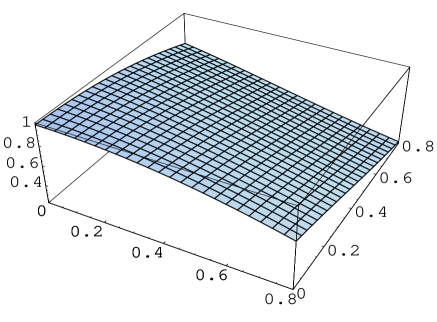
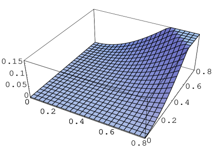
Figure 1: The entanglement of the generated entangled channels from a system initially prepared in maximum entangled state (MES) between:(a) Alice and Rob in the first region $\rho_{\tilde{A}_{I}\tilde{R}_{I}}$, (b) Alice and Rob in the second region $\rho_{\tilde{A}_{II}\tilde{R}_{II}}$, (c) Alice and Anti-Rob $\rho_{\tilde{A}_{I}\tilde{R}_{II}}$, (d) Rob and anti-Alice, $\rho_{\tilde{R}_{I}\tilde{A}_{II}}$.

In this section, we investigate the entanglement behavior for different classes of initial states settings. The earliest investigation has considered only one qubit moving with a uniform acceleration while the other one stays stationary [7]. In the current study, we investigate extensively all different situations.

To measure the entanglement of the generated entangled channels between the qubits and their Anti-qubits, we use Wotters’concurrence [16],

$$\mathcal{C}=\max\Bigl{\{}0,\lambda_{1}-\lambda_{2}-\lambda_{3}-\lambda_{4}\Bigr{\}},$$ (33)

where $\lambda_{1}\geq\lambda_{2}\geq\lambda_{3}\geq\lambda_{4}$ and $\lambda_{i}$ are the eigenvalues of the density operator $\rho=\sigma_{y}\tau_{y}\rho^{*}\sigma_{y}\tau_{y}$, $\rho^{*}$ is the complex conjugate of $\rho$.

Fig.(1), shows the dynamics of the concurrence $\mathcal{C}$ for a system initially prepared in maximum entangled state. In this investigation we assume that both qubits are equally accelerated i.e., $r_{a}=r_{b}=r$. Fig.(1a) displays the dynamics of the concurrence $\mathcal{C}$ of the generated entangled channel between Alice and Rob in the first region $\rho_{\tilde{A}_{I}\tilde{R}_{I}}$. It is clear that, since we start with MES ,the concurrence $\mathcal{C}=1$ at $r_{a}=r_{b}=0$. However if, the first qubit is accelerated while the second qubit stays stationary i.e., $r_{a}=r$ and $r_{b}=0$, then the concurrence decreases smoothly and gradually and does’nt vanish even when the acceleration tends to infinity. However, if the second qubit is also accelerated, then the concurrence decreases faster and vanishes completely at infinity.

Fig.(1b) displays the concurrence dynamics of the generated channel between Alice and Rob in the second region $\rho_{\tilde{A}_{II}\tilde{R}_{II}}$. It is clear that, the system is disentangled for small values of the accelerations. However an entangled channel is generated between Alice and Rob in the second region with $\mathcal{C}\leq 0.15$.

In Fig.(1c), we quantify the degree of entanglement which is generated between Alice (in the first region $I$) and Anti-Rob (in the second region $II$). This figure displays that the maximum value of $\mathcal{C}=0.4$, is reached for zero acceleration of both qubits. However if only one qubit is accelerated, then the evolved channel between Alice and Rob becomes separable. As soon as the second qubit is accelerated, an entangled channel is generated between Alice and Anti-Rob, $\rho_{\tilde{A}_{I}\tilde{R}_{II}}$. The concurrence of this channel increases as the acceleration of Rob’s particle increases. The concurrence of the generated channel between Rob and Anti-Alice is depicted in Fig.(1d). It is clear that, this channel is separable for zero accelerations. However as soon as the acceleration of Alice increases an entangled channel is generated. The maximum value of the concurrence of this channel is $\mathcal{C}\leq 0.4$.

Fig.(2) displays the dynamics of the concurrence $\mathcal{C}$ for a Werner class and a generalized Werner state. Fig.(2a) describes the concurrence dynamics of the generated channel between Alice and Rob in the first region, $\rho_{\tilde{A}_{I}\tilde{R}_{I}}$ where it is assumed that both qubits are accelerated. At zero accelerations ($r_{a}=r_{b}=0$), the concurrence depends on the initial degree of entanglement. The entanglement decays smoothly and gradually as soon as any qubit is accelerated. However, the entanglement decays faster when both qubits are accelerated and completely vanishes at infinite accelerations. Fig.(2b) shows the behavior of the entanglement for the generalized Werner state where we set $c_{x}=0.7,c_{y}=0.5$ and $c_{z}=0.3$. This figure displays a similar behavior as that shown in Fig.(2a) at zero acceleration. For large accelerations the entanglement decreases suddenly to reach its minimum values. Theses minimum values increase for larger accelerations of both qubits.

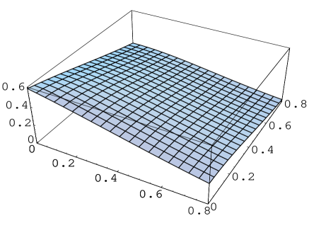
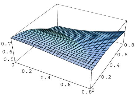
Figure 2: The entanglement of the generated state between Alice and Rob, $\rho_{A_{I}R_{I}}$for (a) Werner state with $x=0.6$, (b) generalized Werner state with $c_{x}=0.7,c_{y}=0.5,c_{z}=0.3$.

Fig.(3), describes the concurrence dynamics of a travelling state initially prepared in the generic pure state (29),where we consider that both qubits are accelerated with the same acceleration. It is clear that at $p=0$, namely, the initial system is MES, the concurrence is maximum $(\mathcal{C}=1)$. As the accelerations of both qubits increase, the concurrence decreases gradually. For larger values of $p$ (i.e. the initial system is partially entangled), the concurrence decreases gradually and completely vanishes at $p=1$.

From Figs.(1) and (2), one can conclude some important results: first the entanglement of the generated channels depends on the initial entanglement of the travelling state. Second, the generated channel in the second region behaves classically and non-classically for small range of finite accelerations. Third, the entanglement between one qubit and the Anti-of the second qubit depends on the acceleration of the Anti particle. Fourth, the generalized Werner state is the most robust type of the self transposed classes. Fifth, among all theses classes the generic pure state is more robust than the self transposed classes even the travelling sate is maximum entangled.

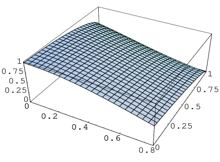
Figure 3: (a) The degree of entanglement of a system is initially prepared in a generic pure state, where it is assumed that the two qubits are accelerated i.e. $r_{a}=r_{b}=r$

5 Usefulness classes

In this section, we investigate the usefulness of the different classes from two different points of view. First, we quantify the fidelity $\mathcal{F}=tr\Bigl{\{}\rho_{\mathrm{final}}\rho_{\mathrm{initial}}\Bigr{\}}$ of the travelling channel in the different regions [17]. Second we investigate the possibility of using the travelling channels to perform the original quantum teleportation [18].

1. Fidelities of the travelling states

   Let us first consider that the travelling channel is prepared initially in a class of self transposed states (8). For this class, the fidelity $\mathcal{F}_{I}$ of the travelling state in the first region is given by,

   $$\mathcal{F}_{I} = \frac{1+C_{zz}}{4}\Bigl{\{}\varrho_{11}\mathcal{C}_{1}^{2}\mathcal{C}_{2}^{2}+\mathcal{\varrho}_{44}\Bigr{\}}+\frac{C_{xx}+c_{yy}}{2}(\varrho_{23}+\varrho_{32})\mathcal{C}_{1}\mathcal{C}_{2}$$

   $$+ \frac{C_{xx}-C_{yy}}{4}(\varrho_{14}+\varrho_{41})\mathcal{C}_{1}\mathcal{C}_{2}+\frac{1-C_{zz}}{4}\Bigl{\{}\mathcal{C}_{1}^{2}(\varrho_{22}+\varrho_{11}\mathcal{S}_{2}^{2})+\mathcal{C}_{2}^{2}(\varrho_{33}+\varrho_{11}\mathcal{S}_{1}^{2})\Bigr{\}},$$

   while, the fidelity of the travelling channel in the region $II$ is,

   $$\mathcal{F}_{II} = \frac{1+C_{zz}}{4}\Bigl{\{}\varrho_{11}\mathcal{S}_{1}^{2}\mathcal{S}_{2}^{2}+\mathcal{\varrho}_{11}\Bigr{\}}+\frac{C_{xx}+c_{yy}}{2}(\varrho_{23}+\varrho_{32})\mathcal{S}_{1}\mathcal{S}_{2}$$

   $$+\frac{C_{xx}-C_{yy}}{4}(\varrho_{14}+\varrho_{41})\mathcal{S}_{1}\mathcal{S}_{2}+\frac{1-C_{zz}}{4}\Bigl{\{}\mathcal{S}_{2}^{2}(\varrho_{33}+\varrho_{11}\mathcal{C}_{1}^{2})+\mathcal{S}_{1}^{2}(\varrho_{22}+\varrho_{11}\mathcal{C}_{1}^{2})\Bigr{\}}.$$

   Similarly, one can obtain a form of the fidelity of the channels between Alice and Anti-Rob, $\rho_{\tilde{A}_{I}\tilde{R}_{II}}$ and between Rob, Anti-Alice $\rho_{\tilde{R}_{I}\tilde{A}_{II}}$.

   

   

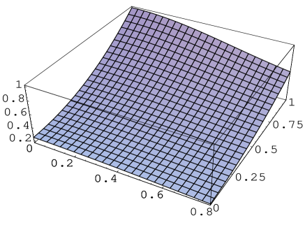
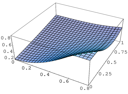
   Figure 4: The Fidelity of the travelling state between: (a) Alice and Rob, $\rho_{\tilde{A}_{I}\tilde{R}_{I}}$, (b) Alice and Rob in the second region $\rho_{A_{II}R_{II}}$, (c) Alice and Anti-Rob, $\rho_{\tilde{A}_{I}\tilde{R}_{II}}$, (d) Rob and Anti-Alice, $\rho_{\tilde{R}_{I}\tilde{A}_{II}}$, where it is assumed that both particles are accelerated i..e $r_{a}=r_{b}=r$ for a system initially prepared in a self transposed type(MES or Werner).

   The dynamics of the fidelities is described in Fig.(4), where it is assumed that both qubits are accelerated with the same acceleration i.e. $r_{a}=r_{b}=r$. This class of state represents the maximum entangled state($x=1$) and different classes of Werner states for ($0<x<1$). Fig.(4a) displays the dynamics of $\mathcal{F}_{I}$ for different classes of self transposed states. Let us consider the first class which is described by $c_{xx}=c_{yy}=c_{zz}=x$ where $x\in[0,0.20]$. For this class, the fidelity $\mathcal{F}\in[0,0.2]$, where the largest value is reached at $r=0$ and the smallest value is reached at infinite acceleration i.e $r=\frac{\pi}{4}$. For the second class which includes all classes with $x\in(0.2,1.0)$, the fidelity $\mathcal{F}_{I}$, increases for small values of $r$ and larger values of $x$. For the second class the fidelity is better than the first one even for larger values of $r$. Finally for the third class with $x=1$, which represents the maximum entangled class, the fidelity $\mathcal{F}$ is maximum for $r=0$ and $x=1$. However as $r$ increases the fidelity of the travelling state is the best one, where $\mathcal{F}\in[0.8,1]$.

   Fig.(4b) shows the behavior of the fidelity in the second region $\mathcal{F}_{II}$ for different classes of the self transposed states which are characteristic by the parameter $x$. The fidelity is almost zero for small values of $r$ and $x$, i.e. initially the travelling states have a smaller degree of entanglement. As $x$ increases, the maximum fidelity $\mathcal{F}_{II}\in[0,0.4]$ and increases slightly for larger values $(x=1)$.

   The fidelity of the generated channel between Alice and Anti-Rob, $\rho_{\tilde{A}_{I},\tilde{R}_{II}}$ is displayed in Fig.(4c). It is clear that the fidelity decreases as one increases the acceleration of both qubits. However for larger values of the parameter $x$, the fidelity decreases faster and almost vanishes for maximum entangled state. i.e., at $x=1$. The dynamics of the fidelity between Rob and ant-Alice is depicted in Fig.(4d). The behavior of the fidelity is similar to that shown in Fig.(4c), but the maximum fidelity is smaller and decreases faster for larger values of the accelerations and the parameter $x$.

   Now, we consider the dynamics of the fidelity for a system initially prepared in a generic pure state (29). For this class, the fidelity of the travelling channel in the first region $I$ is given by,

   $$\mathcal{F}_{I}^{\mathrm{p}}=(\frac{1-q}{4})^{2}\left\{\mathcal{C}_{1}^{2}\mathcal{C}_{2}+2\mathcal{C}_{1}\mathcal{C}_{2}+\mathcal{S}_{1}^{2}\mathcal{S}_{2}^{2}+1\right\}+(\frac{1+q}{4})^{2}(\mathcal{C}_{1}+\mathcal{C}_{2})^{2}+(\frac{p}{4})^{2}(4\mathcal{C}_{2}+2\mathcal{C}_{1}),$$ (36)

   while in the second region $II$, it is given by,

   $$\mathcal{F}^{\mathrm{p}}_{II} = \left(\frac{1+q}{4}\right)^{2}\Bigl{[}1+2\mathcal{S}_{1}\mathcal{S}_{2}+\mathcal{C}_{1}^{2}\mathcal{C}_{2}^{2}+\mathcal{S}_{1}^{2}\mathcal{S}_{2}^{2}\Bigr{]}+\left(\frac{1+q}{4}\right)^{2}(\mathcal{S}_{1}+\mathcal{S}_{2})^{2}++\frac{p^{2}}{4}(\mathcal{S}_{1}+\mathcal{S}_{2})$$ (37)

   $$+ \frac{1-q^{2}}{16}\left(\mathcal{C}_{1}^{2}+\mathcal{C}_{2}^{2}+\mathcal{C}_{1}^{2}\mathcal{S}_{2}^{2}+\mathcal{S}_{1}^{2}\mathcal{C}_{2}^{2}\right).$$

   

   

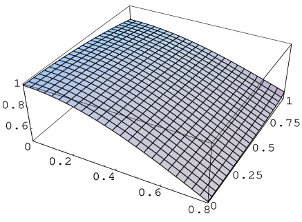
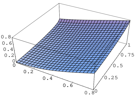
   Figure 5: The Fidelity of the travelling state , where it is assumed that both particles are accelerated i.e, $r_{a}=r_{b}=r$ for a system initially prepared in a pure state,(a) for the first region $I$ and (b) for the second region $II$.

   The dynamic of the fidelity for a system initially prepared in the generic pure state (29) is displayed in Fig.(5). In the first region, the fidelity $\mathcal{F}_{I}$ is shown in Fig.(5a). It is clear that at $p=0$ i.e., the travelling state is maximum entangled channel ($\mathcal{F}^{\mathrm{p}}_{I}=1$) at $r=0$. For larger $p$ and smaller $r$, the fidelity decreases slightly. However the fidelity decreases smoothly and gradually for larger values of $r$ and completely vanishes at infinity. Fig.(5b) describes the behavior of the fidelity of the travelling state in the second region $\mathcal{F}^{\mathrm{p}}_{II}$. For small values of $r$ and even larger values of $p$, the fidelity is very small. However as $r$ increases, the fidelity increases smoothly and reaches its upper bound at $p=1$.

2. Usefulness classes for teleportation

   

   

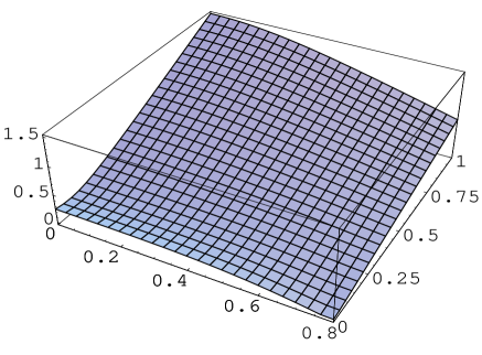
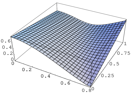
   Figure 6: The teleportation inequality (38) of the travelling channel, where it is assumed that both particles are accelerated i.e., $r_{a}=r_{b}=r$ in the first region $I$ for a system initially prepared in a self transposed type(MES or Werner) for (a) $\rho_{\tilde{A}_{I}\tilde{R}_{I}}$, (b)$\rho_{\tilde{A}_{II}\tilde{R}_{II}}$, (c) $\rho_{\tilde{A}_{I}\tilde{R}_{II}}$ and (d) $\rho_{\tilde{R}_{I}\tilde{A}_{II}}$.

   To examine wether the travelling state can be used as a quantum channel to implement teleportation, we use Hordecki’s criterion [19]. This criterion state that any mixed spin $\frac{1}{2}$ state is useful for quantum teleportation if $tr\sqrt{~{}\mathord{\begin{picture}(12.0,12.0)(-1.0,0.0)\put(-3.0,12.0){\makebox(0.0,0.0)[t]{$\scriptscriptstyle\downarrow$}} \put(-3.0,13.0){\makebox(0.0,0.0)[l]{$\scriptscriptstyle\longrightarrow$}} \put(5.0,0.0){\makebox(0.0,0.0)[b]{$C$}} \end{picture}}^{T}~{}\mathord{\begin{picture}(12.0,12.0)(-1.0,0.0)\put(-3.0,12.0){\makebox(0.0,0.0)[t]{$\scriptscriptstyle\downarrow$}} \put(-3.0,13.0){\makebox(0.0,0.0)[l]{$\scriptscriptstyle\longrightarrow$}} \put(5.0,0.0){\makebox(0.0,0.0)[b]{$C$}} \end{picture}}~{}}>1.$ The self transposed states are useful for quantum teleportation if,

   $$Telp=\sqrt{\tilde{C}^{2(i)}_{xx}+\tilde{C}_{yy}^{2(i)}+\tilde{C}_{zz}^{2(i)}}>1,$$ (38)

   where $i=I,II$ for the first and second regions respectively. Fig.(6), shows the possibility of using the travelling state as quantum channel between two users to perform the quantum teleportation protocol. In Fig.(6a), we consider that the users initially share a maximum entangled state or Werner state. it is clear that, for small values of $r$ and small values of $x$ the teleportation inequality $\mathrm{Telp}<1$. However as $x$ increases while the acceleration $r$ is small, the possibility of using the channel for quantum teleportation increases. For larger values of $r$ and smaller values of $x$, i.e., the system is of Werner type with small degree of entanglement, $\mathrm{Telp}<1$ and consequently the channel is useless for quantum teleportation. As $x$ increases (we increases the degree of entanglement), the quantum channel is useful for quantum teleportation even for larger values of $r$.

   Fig.(6c) describes the behavior of the Horodecki’s criterion for the generated entangled channel between Alice and Anti-Rob. It is clear that, the maximum value of the inequality (40) is smaller than one ( $\mathrm{Telp}<1$) for all self transposed classes. Therefore according to Horodecki’s criterion, this channel is useless for quantum teleportation. Also for the generated entangled channel between Rob and Anti-Alice, Horodeciki’s inequality is violated and consequently this class can not be used as a quantum channel to perform quantum teleportation as shown in Fig.(6d).

   Fig.(7), displays the Horodecki’s inequality (40) for a system initially prepared in the generic pure state (29). It is clear that for MES, namely $p=0$, the travelling channel can be used as a quantum channel to perform quantum teleportatiion $(Telp>1)$ for $r\sim\in[0,4]$. However for larger values of $p\in[0,0.75]$ and smaller values of $r$, the travelling channel obeys Horedicki’s inequality (38) and consequently all these classes could be used to implement the quantum teleportation protocol. Finally the last classes which are characteristic by $p\in[0.75,1]$ violate the teleportation inequality (38) and consequently this classes could not be used as quantum channels to perform teleportation.

   

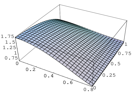
   Figure 7: The teleportation inequality (38) of the travelling state , where it is assumed that both particles are accelerated i.e., $r_{a}=r_{b}=r$ in the first region $I$ for a system prepared initially in a generic pure state (30).

   From these results, one concludes that it is possible to generate entangled channels between Alice, Rob in the first and second regions, Alice, Anti-Rob, and between Rob, Anti-Alice. For MES, the largest entanglement can be generated between Alice and Rob $\rho_{\tilde{A}_{I}\tilde{R}_{I}}$ in the first region and the smallest values of entanglement contained in $\rho_{\tilde{A}_{II}\tilde{R}_{II}}$. The generalized Werner state is more robust than the MES and Werner classes. However the pure states which represent a class of partial entangled states are more robust than the self transposed class. The possibility of using the pure state for quantum teleportation proposes are much better than the other classes.

6 Conclusion

An analytical solution for a general two qubits system of Dirac fields in noninertial frame is introduced. The density operator of the travelling channels between the observers and their Anti-observers are calculated. Two particular classes are investigated extensively: the self transposed class, which includes the maximum entangled state and all classes of Werner states and a class of a generic pure state of a two qubits system .

For the self transposed states (MES or Werner) the degree of entanglement in all different generated states depends on the entanglement of the initial travelling state. The degree of entanglement decreases smoothly if only one qubits accelerated and it vanishes completely if the acceleration of at least one qubit tends to infinity. However, the entanglement vanishes faster for less initial entangled states. For a general class of generalized Werner state, the entanglement doesn’t vanish even for larger accelerations. Starting from a generic pure state, the entanglement is more robust than that depicted for the self transposed classes, where the entanglement decreases slowly and gradually. For this class, we show that, an entangled channels in the second region with small degree of entanglement is generated.

We distinguish between the usefulness of the travelling classes by investigating two phenomena:first, we quantify the fidelity of the travelling channels in the two regions and the second, the possibility of using the travelling channels as quantum channels to perform the quantum teleportation. The fidelity of the travelling channels depends on the entanglement of the initial state, where it is larger for higher entanglement. For the self transposed states, the fidelity is maximum for maximum entangled state and decreases smoothly as the acceleration of any particle increases. For less entangled states, the fidelity is smaller and decreases faster. In the second region, the fidelity of the travelling channel increases gradually and it is smaller for the maximum entangled state comparing with that in the first region. On the other hand, the entanglement of the generated entangled channels between Alice and Anti-Rob is much larger than that depicted between Alice and Rob in the second region.

The fidelity of a travelling channel starting from a generic pure state is investigated in both regions, where the fidelity of this class is much better than that depicted for the self transposed classes. In the first region, the loss of the fidelity is very small for the smallest entanglement of initial classes. On the other hand, the fidelity of the generic pure state in the second region is much better than its corresponding one for the self transposed class.

The usefulness of the travelling channels is investigated for different classes. We showed that it is possible to use some classes of the self transposed states for quantum teleportation. These classes are generated from a system that has an initial degree of entanglement ($>0.5$) and its qubits are accelerated with an acceleration $<0.6$). On the other hand, starting from a generic pure state with smaller values of its parameter, one can generate entangled channels in the first region useful for quantum teleportation with larger acceleration

In conclusion, the possibility of generating entangled channels in both regions depends on the degree of entanglement of the initial travelling state. The fidelity and the usefulness of the generic pure state is much better than that depicted for the self transposed classes. Therefore, one can say that the generic pure state is more robust than the self transposed classes.

References

• [1] D. Bouwmeesterm A. Ekert, A. Zeilinger, ” The physics of quantum Information”, Springer-verlag (200).
• [2] T. P. Spiller, Kae Nemoto, Samuel L. Braunstein, W. J. Munro, P. van Loock, G. J. Milburn, New J. Phys. 8, 30 (2006), R. Horodecki, P. Horodecki,M. Horodecki and K. Hprodecki, Rev. Mod. Phys. 81 865 (2009).
• [3] P. M. Alsing, I. F. Schuller, R. B. Mann and T. E. Tessier, Phys. Rev. A 74 032326 (2006).
• [4] D. E. Bruschi, J. Louko, E. Martn-Martnez, A. Dragan, and I. Fuentes, Phys. Rev. A 82 042332 (2010);M. Aspachs, G. Adesso, and I. Fuentes, Phys. Rev. Lett 105 , 151301 (2010); E. Mart n-Mart nez, L. J. Garay and Juan Le on, Phys. Rev. D 82, 064006 (2010).
• [5] Andre G. S. Landulfo, George E. A. Matsas, Phys. Rev.A80, 032315, (2009); L. C. Celeri, A. G. S. Landulfo, R. M. Serra, G. E. A. Matsas, Phys. Rev. A 81, 062130 (2010).
• [6] H. M. Dehnavi, B. Mirza, H. Mohammadzadeh and R. Rahimi, Annals of Phys. 326 1320 (2011).
• [7] J. Wang and J. Jing, Phys. Rev. A. 83 022314 (2011).
• [8] M. Montero, J.Le$\grave{o}$n and E. M.- Mart$\grave{i}$nez, Phys. Rev. A 84,042320 (2011).
• [9] D. E. Bruschi, J. Louko, E. Martn-Martnez, A. Dragan, and I. Fuentes, Phys. Rev. A 82 042332 (2010);M. Aspachs, G. Adesso, and I. Fuentes, Phys. Rev. Lett 105 , 151301 (2010); E. Mart n-Mart nez, L. J. Garay and Juan Le on, Phys. Rev. D 82, 064006 (2010).
• [10] N. Metwally, ”Entangled qubit pairs” , Dissertation an der Fakult$\ddot{a}$t f$\ddot{u}$r Physik der. Ludwig- Maximilians-Universit$\dot{a}$t M nchen (2002).
• [11] B.-G. Englert and N. Metwally, J. Mod. Opt. 47, 221 (2000);B.-G. Englert and N. Metwally, Appl. Phys B72, 35 (2001).
• [12] T. Yu and J. H. Eberly, Quantum Inform. Comput. 7, 459 (2007);A. R. P. Rau, J. Phys. A 42, 412002 (2009).
• [13] S. Hill and W. K. Wootters, Phys. Rev. Lett. 78, 5022 (1997).
• [14] Jieci Wang, Jiliang Jing, quantum-ph. arXiv:1105.1216 (2011).
• [15] R. F. Werner, Phys. Rev. A 40, 4277 (1989).
• [16] S. Hill and W. K. Wootters, Phys. Rev. Lett. 78 5022 (1997); W. K. Wootters W K, Phys. Rev. Lett. 80 2245 (1998).
• [17] C.-Ping Yang, phys. Rev. A82 054303 (2010); R. Ronke, T. Spiller, I. D’Amico, J. Phys.: Conf. Ser-286 012020 (2011).
• [18] C. H. Bennett, G. Brassard, C. Crepeau, R. Jozsa, A. Pweres and W. K. Wootters, Phys. Rev. Lett. 70 1895 (1993).
• [19] P. Horodecki, Phys. Lett. A232 333 (1997).