Observational tests of inflation with a field derivative coupling to gravity

Abstract

A field kinetic coupling with the Einstein tensor leads to a gravitationally enhanced friction during inflation, by which even steep potentials with theoretically natural model parameters can drive cosmic acceleration. In the presence of this non-minimal derivative coupling we place observational constraints on a number of representative inflationary models such as chaotic inflation, inflation with exponential potentials, natural inflation, and hybrid inflation. We show that most of the models can be made compatible with the current observational data mainly due to the suppressed tensor-to-scalar ratio.

I Introduction

Inflation has been the backbone of the high-energy cosmology over the past 3 decades infpapers . The most simple source for inflation is a minimally coupled scalar field $\phi$ (“inflaton”) with a slowly varying potential $V(\phi)$ newinf ; chaotic The spectra of density perturbations generated from the quantum fluctuations of inflaton are consistent with the temperature anisotropies observed in the Cosmic Microwave Background (CMB) infper .

From the amplitude of the observed CMB anisotropies COBE ; WMAP7 the typical mass scale of inflation is known to be around $m\sim 10^{14}$ GeV Liddle . This is much larger than the electroweak scale ($\sim 10^{2}$ GeV), which suggests the requirement of new physics beyond the Standard Model of particle physics Riotto . In other words, for the potential $V(\phi)=(\lambda/4)(\phi^{2}-v^{2})^{2}$ with $v\sim 10^{2}$ GeV, the coupling $\lambda$ is constrained to be $\lambda\sim 10^{-13}$ from the CMB normalization Liddle , but this is much smaller than the coupling constant $\lambda\sim 0.1$ of the Higgs boson particlereview .

There have been attempts to accommodate the Higgs field for inflation. One is to use a non-minimal field coupling $\xi R\phi^{2}/2$ with the Ricci scalar $R$ Bezrukov (see also Refs. Maeda ). If $\xi\gg 1$ the self coupling $\lambda$ can be as large as $\lambda\approx 10^{-10}\xi^{2}$ from the CMB normalization Salopek . Although this scenario is attractive, it is plagued by the unitary-violation problem associated with graviton exchange in $2\to 2$ scalar scattering around the energy scale $\Lambda_{c}\approx M_{\rm pl}/\xi$ (where $M_{\rm pl}=2.44\times 10^{18}$ GeV is the reduced Planck mass) Burgess . Since $\Lambda_{c}$ is around the energy scale of inflation, some strong coupling effect can give rise to additional corrections to the inflaton potential.

Another attempt is to employ a field derivative coupling with the Einstein tensor $G^{\mu\nu}$, i.e. $G^{\mu\nu}\partial_{\mu}\phi\partial_{\nu}\phi/(2M^{2})$, where $M$ is a constant having a dimension of mass Germani1 (see also Ref. Amendola for the original work). In the regime where the Hubble parameter $H$ is larger than $M$ the field evolves more slowly relative to the case of standard inflation due to a gravitationally enhanced friction. Hence it is possible to reconcile steep potentials such as $V(\phi)=\lambda\phi^{4}/4$ ($\lambda\sim 0.1$) with the CMB observations.

In Refs. Germani1 ; Germaniper ; Germani2 ; Watanabe ; Germani11 it was shown that, for a slow-rolling scalar field satisfying the condition $\varepsilon\equiv(\partial\phi)^{2}/(M^{2}M_{\rm pl}^{2})\ll 1$, the strong coupling scale $\Lambda_{c}$ of the derivative coupling theory is around $M_{\rm pl}$ in a homogeneous and isotropic cosmological background. Provided that $H$ and $M$ are below the Planck scale, the theory is in a weak coupling regime with suppressed quantum corrections.

The property of the high cut-off scale $\Lambda_{c}$ around $M_{\rm pl}$ is associated with the fact that whenever the non-minimal derivative coupling to gravity dominates over the canonical kinetic term the theory possesses an asymptotic local shift symmetry for $\varepsilon\ll 1$ Germani11 . This symmetry is related to the Galilean symmetry $\phi\to\phi+c+c_{\mu}x^{\mu}$ in Minkowski space-time Nicolis , but the difference is that the coordinate $x^{\mu}$ in the derivative coupling theory on curved backgrounds is linked to the covariantly constant Killing vectors Germani11 . In the presence of a slowly varying inflaton potential such a local symmetry is only softly broken, so that the potential can be protected against quantum corrections during inflation. The field self-interaction of the form $(\partial\phi)^{2}\square\phi$ Nicolis ; covaga , which satisfies the Galilean symmetry in the limit of Minkowski space-time, also leads to the slow evolution of $\phi$ along the inflaton potential Kamada (see also Refs. Galileoninf ).

A nice feature of the non-minimal derivative coupling with the Einstein tensor is that the mechanism of the gravitationally enhanced friction works for general steep potentials. For instance, let us consider the potential of natural inflation, $V(\phi)=\Lambda^{4}[1+\cos(\phi/f)]$, where $f$ characterizes the scale of the breaking of a global shift symmetry Freese . In order for this potential to be consistent with the CMB observations, we require that $f$ is larger than $3.5M_{\rm pl}$ in conventional slow-roll inflation Savage . Then the global symmetry is broken above the quantum gravity scale, in which case quantum field theory may be invalid naturalpro . In the presence of the non-minimal derivative coupling to gravity, however, the scale $f$ can be much smaller than $M_{\rm pl}$ because of the gravitationally enhanced friction Germani2 ; Watanabe .

Another example is the exponential potential $V(\phi)=V_{0}e^{\beta\phi/M_{\rm pl}}$, whose dominance leads to the power-law expansion of the Universe (with the scale factor $a\propto t^{2/\beta^{2}}$, where $t$ is cosmic time) earlyexp . In higher-dimensional gravitational theories, exponential potentials often arise as the curvature of internal spaces related with the geometry of extra dimensions expmoti . In such cases the constant $\beta$ is usually larger than the order of unity, so that it is difficult to realize sufficient amount of inflation. As we will see later, this problem can be circumvented by taking into account the non-minimal derivative coupling. Moreover, unlike the standard case, inflation comes to end with gravitational particle production.

In order to test the viability of inflationary models with the non-minimal derivative coupling it is important to estimate the power spectra of density perturbations relevant to the CMB anisotropies. In Refs. Germaniper ; Watanabe the authors computed the inflationary observables such as the scalar spectral index $n_{\rm s}$, the tensor-to-scalar ratio $r$, and the nonlinear parameter $f_{\rm NL}^{\rm equil}$ of the equilateral scalar non-Gaussianities (see also Refs. KYY ; Gao ; DT11 ). Since the scalar propagation speed is close to the speed of light during inflation, the scalar non-Gaussianities are suppressed to be small ($|f_{\rm NL}^{\rm equil}|\ll 1$). Hence $n_{\rm s}$ and $r$ are the two main observables to distinguish between different inflaton potentials.

In this paper we shall place observational constraints on a number of representative inflationary models in the presence of the field derivative coupling with the Einstein tensor. We use the bounds derived from the joint data analysis of WMAP7 WMAP7 , Baryon Acoustic Oscillations (BAO) BAO , and the Hubble constant measurement (HST) HST . Note that some constraints on Higgs inflation and natural inflation have been discussed in Refs. Germaniper ; Watanabe without the CMB likelihood analysis. In Ref. Popa the author carried out the cosmological Monte-Carlo simulation to test Higgs inflation with the field derivative coupling to gravity. Our analysis based on the recent observational data is general enough to cover a wide variety of models such as chaotic inflation chaotic , inflation with exponential potentials earlyexp , natural inflation Freese , and hybrid inflation hybrid . We show that the gravitationally enhanced friction mechanism can make most of the models compatible with the current observations.

II Background dynamics

We start with the following 4-dimensional action

$$S=\int d^{4}x\sqrt{-g}\left[\frac{M_{\rm pl}^{2}}{2}R-\frac{1}{2}\Delta^{\mu\nu}\partial_{\mu}\phi\partial_{\nu}\phi-V(\phi)\right]\,,$$ (1)

where

$$\Delta^{\mu\nu}=g^{\mu\nu}-\frac{1}{M^{2}}G^{\mu\nu}\,.$$ (2)

Here $g$ is a determinant of the space-time metric $g_{\mu\nu}$, $R$ is the Ricci scalar, $G^{\mu\nu}$ is the Einstein tensor, $M$ is a constant having a dimension of mass, and $V(\phi)$ is the potential of a scalar field $\phi$.

The action (1) belongs to a class of the most general scalar-tensor theories having second-order equations of motion (which is required to avoid the Ostrogradski instability) Horndeski ; Deffayet ; Char ; KYY . The Lagrangian in such general Horndeski’s theories is the sum of the terms ${\cal L}_{2}=K(\phi,X)$, ${\cal L}_{3}=-G_{3}(\phi,X)\square\phi$, ${\cal L}_{4}=G_{4}(\phi,X)R+G_{4,X}\times[{\rm field\leavevmode\nobreak\ derivative\leavevmode\nobreak\ terms}]$, and ${\cal L}_{5}=G_{5}(\phi,X)G^{\mu\nu}(\nabla_{\mu}\nabla_{\nu}\phi)-(G_{5,X}/6)\times[{\rm field\leavevmode\nobreak\ derivative\leavevmode\nobreak\ terms}]$, where $K$, $G_{i}$ ($i=3,4,5$) are functions of $\phi$ and $X=-g^{\mu\nu}\partial_{\mu}\phi\partial_{\nu}\phi/2$, and $G_{i,X}=\partial G_{i}/\partial X$ Deffayet ; KYY . The conditions for the avoidance of ghosts and Laplacian instabilities were derived in Refs. KYY ; DTjcap . These conditions can be used to restrict the functional forms of $K$, $G_{i}$ ($i=3,4,5$) to construct theoretically consistent models of inflation.

The non-minimal derivative coupling in Eq. (1) is recovered in the Horndeski’s Lagrangian by choosing the function $G_{5}=-\phi/(2M^{2})$ after integration by parts. The sign in front of the term $G^{\mu\nu}/M^{2}$ in Eq. (2) is chosen to avoid the appearance of ghosts in the scalar sector Germani1 ; Germani2 .

In Ref. Germani11 it was found that in a manifold having integrable (covariantly constant) Killing vectors $\xi^{a}$ the field Lagrangian $-\Delta^{\mu\nu}\partial_{\mu}\phi\partial_{\nu}\phi/2$ in Eq. (1) is invariant under the (curved-space) Galilean transformation $\phi(x)\to\phi(x)+c+c_{a}\int^{x}_{x_{0}}\xi^{a}$, where $c$, $c_{a}$, $x_{0}$ are constants and $x$ is a space-time coordinate. The existence of the Galilean symmetry has an advantage that the theory can be quantum mechanically under control Trod .

Imposing the above Galilean symmetry in the curved background with integrable Killing vectors, Germani et al. Germani11 showed that the second-order Lagrangians are restricted to take the forms $-\Delta^{\mu\nu}\partial_{\mu}\phi\partial_{\nu}\phi/2$ or $X\square\phi$ (plus a field derivative coupling with the double dual Riemann tensor). In the small derivative regime in which the condition $(\partial\phi)^{2}/(M^{2}M_{\rm pl}^{2})\ll 1$ is satisfied (e.g., during inflation), an approximate infinitesimal shift symmetry $\phi\to\phi+f(x)$ (where $f(x)$ is an arbitrary function of space-time coordinates $x$) emerges for the Lagrangian $G^{\mu\nu}\partial_{\mu}\phi\partial_{\nu}\phi/(2M^{2})$, provided that the metric is shifted appropriately Germani11 . The existence of such a gauge symmetry can allow the theory (1) to be protected against quantum corrections even up to the Planck scale. Note that the term $X\square\phi$ does not possess such a general gauge shift symmetry.

The scale of unitarity violation for the theory (1) was estimated in Ref. Germani1 in the context of Higgs inflation. In Standard Model we can consider the $\phi\phi\to\phi\phi$ scattering via graviton exchange, where $\phi$ is one of the real scalar degrees of freedom for the Higgs doublet. We expand the metric in the form $g_{\mu\nu}=g_{\mu\nu}^{(0)}+h_{\mu\nu}/M_{\rm pl}$, where $g_{\mu\nu}^{(0)}=(-1,a^{2}(t),a^{2}(t),a^{2}(t))$ is the metric on the flat Friedmann-Lemaître-Robertson-Walker (FLRW) background ($a(t)$ is the scale factor with cosmic time $t$). We are interested in the high-friction regime in which the Hubble parameter $H=\dot{a}/a$ (a dot represents a derivative with respect to $t$) is much larger than $M$. In this regime the field $\phi$ is expanded as $\phi=\phi_{0}+M\chi/(\sqrt{3}H)$, where $\chi$ is a canonically normalized field perturbation. The first non-renormalizable operator associated with the interaction between gravitons and scalars is given by Germani1

$$I=\frac{1}{2H^{2}M_{\rm pl}}\partial^{2}h^{\mu\nu}\partial_{\mu}\chi\partial_{\nu}\chi\,.$$ (3)

A power counting analysis gives the unitary bound $\Lambda\simeq(2H^{2}M_{\rm pl})^{1/3}$. For the suppression of higher dimensional operators we require the condition $R<\Lambda^{2}$. On using the relation $R\simeq 12H^{2}$ this condition translates into $H<5\times 10^{-2}M_{\rm pl}$, which is satisfied during inflation.

The discussion of the unitary bound given above can be applied to the multi-field inflationary models in which one of the fields is not necessarily responsible for the cosmic acceleration. In single field models where only one field $\phi$ leads to inflation the unitary bound can be as close as the Planck scale $M_{\rm pl}$ in the regime where the condition $(\partial\phi)^{2}/(M^{2}M_{\rm pl}^{2})\ll 1$ is satisfied Watanabe ; Germani11 . In this case the slow-roll evolution of the field $\phi$ suppresses the interaction (3) below the Planck scale.

In the following let us study the background dynamics for the theory described by the action (1). In the flat FLRW background the equations of motion following from the action (1) are

$$3M_{\rm pl}^{2}H^{2}=\frac{1}{2}\dot{\phi^{2}}\left(1+9\frac{H^{2}}{M^{2}}\right)+V(\phi)\,,$$ (4)

$$\frac{1}{a^{3}}\frac{d}{dt}\left[a^{3}\dot{\phi}\left(1+3\frac{H^{2}}{M^{2}}\right)\right]+V_{,\phi}=0\,,$$ (5)

where $V_{,\phi}=dV/d\phi$. In order to solve the dynamical equations numerically, it is convenient to introduce the following dimensionless variables

$$x=\frac{\phi}{M_{\rm pl}}\,,\qquad y=\frac{\dot{\phi}}{MM_{\rm pl}}\,,\qquad z=\frac{H}{M}\,.$$ (6)

Differentiating Eq. (4) with respect to $t$ and using Eq. (5) to eliminate $\dot{H}$, we obtain the second-order equation for the field $\phi$. It then follows that

$$\frac{dx}{d\tau} = y\,,$$ (7)

$$\frac{dy}{d\tau} = -\frac{3yz(2-3y^{2})(1+3z^{2})+(2-y^{2})\hat{V}_{,\phi}(x)}{2(1+3z^{2})+y^{2}(9z^{2}-1)}\,,$$ (8)

$$z = \sqrt{\frac{y^{2}+2\hat{V}(x)}{6-9y^{2}}}\,,$$ (9)

where

$$\tau=Mt\,,\qquad\hat{V}_{,\phi}=\frac{V_{,\phi}}{M^{2}M_{\rm pl}}\,,\qquad\hat{V}=\frac{V}{M^{2}M_{\rm pl}^{2}}\,.$$ (10)

We are interested in slow-roll inflation in which cosmic acceleration is mainly driven by the potential energy $V(\phi)$. In this case Eqs. (4) and (5) reduce to

$$3M_{\rm pl}^{2}H^{2}\simeq V(\phi)\,,$$ (11)

$$3H{\cal A}\,\dot{\phi}+V_{,\phi}\simeq 0\,,$$ (12)

where

$${\cal A}=1+3\frac{H^{2}}{M^{2}}\,.$$ (13)

We define the following slow-roll parameters

$$\epsilon=-\frac{\dot{H}}{H^{2}}\,,\qquad\delta_{\phi}=\frac{\ddot{\phi}}{H\dot{\phi}}\,,$$

$$\delta_{X}=\frac{\dot{\phi}^{2}}{2H^{2}M_{\rm pl}^{2}}\,,\qquad\delta_{D}=\frac{\dot{\phi}^{2}}{4M^{2}M_{\rm pl}^{2}}\,.$$ (14)

For the validity of the slow-roll approximation we require that $\{\epsilon,|\delta_{\phi}|,\delta_{X},\delta_{D}\}\ll 1$. Taking the time-derivative of Eq. (11) and using Eq. (12), we have

$$\epsilon\simeq\delta_{X}+6\delta_{D}\simeq\frac{\epsilon_{{\text{\tiny$V$}}}}{{\cal A}}\,,$$ (15)

where

$$\epsilon_{{\text{\tiny$V$}}}=\frac{M_{\rm pl}^{2}}{2}\left(\frac{V_{,\phi}}{V}\right)^{2}\,.$$ (16)

This shows that $\epsilon\ll\epsilon_{{\text{\tiny$V$}}}$ for ${\cal A}\gg 1$ and hence the evolution of the field $\phi$ slows down relative to that in standard slow-roll inflation.

The field value $\phi_{f}$ at the end of inflation is known by solving $\epsilon(\phi_{f})=1$, i.e.

$$\epsilon_{{\text{\tiny$V$}}}(\phi_{f})\left[1+\frac{V(\phi_{f})}{M^{2}M_{\rm pl}^{2}}\right]^{-1}=1\,.$$ (17)

The number of e-foldings from the time $t$ during inflation to the time $t_{f}$ at the end of inflation is defined by $N=\int_{t}^{t_{f}}H(\tilde{t})\,d\tilde{t}$. On using Eqs. (11) and (12), it follows that

$$N\simeq\frac{1}{M_{\rm pl}^{2}}\int_{\phi_{f}}^{\phi}\left(1+\frac{V}{M^{2}M_{\rm pl}^{2}}\right)\frac{V}{V_{,\tilde{\phi}}}d\tilde{\phi}\,.$$ (18)

If ${\cal A}\gg 1$ (i.e. $H^{2}\gg M^{2}$) during inflation, we can neglect the first term inside the bracket of Eq. (18) relative to the second one. This is not the case for inflation in which the transition from the regime $H>M$ to the regime $H<M$ occurs prior to the onset of reheating.

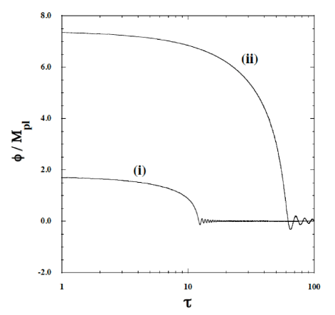
Figure 1: Evolution of the field $\phi$ versus $\tau=Mt$ for (i) $\alpha=100$ and (ii) $\alpha=0.25$. The initial conditions at $N=60$ are chosen by using the slow-roll equations (11) and (12), i.e., (i) $x=1.757$, $y=-0.526$, and (ii) $x=7.397$, $y=-0.521$.

As an example, let us consider chaotic inflation chaotic with the potential

$$V(\phi)=\frac{\lambda}{n}\phi^{n}\,,$$ (19)

where $\lambda$ and $n$ are constants. In this case Eqs. (18) and (17) read

$$N=\frac{x^{2}}{2n}\left[1+\frac{2\alpha}{n(n+2)}x^{n}\right]-\frac{x_{f}^{2}}{2n}\left[1+\frac{2\alpha}{n(n+2)}x_{f}^{n}\right],$$ (20)

$$2x_{f}^{2}\left(1+\frac{\alpha}{n}x_{f}^{n}\right)=n^{2}\,,$$ (21)

where

$$\alpha=\frac{\lambda M_{\rm pl}^{n-2}}{M^{2}}\,,\qquad x_{f}=\frac{\phi_{f}}{M_{\rm pl}}\,.$$ (22)

For the quadratic potential $V(\phi)=m^{2}\phi^{2}/2$ (i.e. $\lambda=m^{2}$ and $n=2$) one has $x_{f}^{2}=(\sqrt{1+4\alpha}-1)/\alpha$ and

$$x^{2}=\left(\sqrt{2+2\sqrt{1+4\alpha}+4\alpha(4N+1)}-2\right)/\alpha\,,$$ (23)

where $\alpha=m^{2}/M^{2}$. In the General Relativistic (GR) limit ($\alpha\to 0$) this gives $x^{2}\to 4N+2$. In the high-friction limit ($\alpha\to\infty$) one has $x^{2}\to 2\sqrt{(4N+1)/\alpha}$, which means that the field value is smaller than that in standard chaotic inflation.

In order to confirm the accuracy of the slow-roll approximation we solve the full equations of motion (7)-(9) numerically. In Fig. 1 the evolution of the field $\phi$ is plotted for the potential $V(\phi)=m^{2}\phi^{2}/2$, i.e. $\hat{V}_{,\phi}=\alpha x$ and $\hat{V}=\alpha x^{2}/2$ in Eqs. (8) and (9). We choose the initial conditions of $x$ and $y$ at $N=60$ by using the values derived under the slow-roll approximation.

The numerical simulations labeled as (i) and (ii) in Fig. 1 correspond to the parameters $\alpha=100$ and $\alpha=0.25$, respectively. In the case (i) the numerical value of $z=H/M$ at the end of inflation ($x_{f}=0.44$) is $z_{f}=2.2$, which means that the solution is in the high-friction regime during inflation. In this case $H$ drops below $M$ at the reheating stage. After inflation there is a transient period with $H>M$ in which the slow-roll condition is violated. In this regime some quantum corrections may come into play to the action (1). As long as such corrections are unimportant in the field equations (4) and (5), we find that the inflaton oscillation is not disturbed during the transient period (see Fig. 1). In the case (ii) we have $z_{f}=0.3$ at $x_{f}=1.3$ and hence the system enters the regime $H<M$ during inflation. In this case the qualitative behavior for the oscillation of inflaton at reheating is not much different from that in standard inflation.

We confirmed that the difference between the numerical and analytic values of the number of e-foldings acquired during inflation is usually less than a few percent. This shows that the slow-roll approximation employed in Eqs. (11) and (12) can be trustable.

III The spectra of density perturbations

The spectra of scalar and tensor perturbations generated in the theories given by the action (1) were derived in Refs. Germaniper ; KYY ; Watanabe ; DT11 . Here we briefly review their formulas in order to apply them to concrete inflationary models in Sec. IV.

The perturbed metric about the flat FLRW background is given by permet

$$ds^{2} = -(1+2A)dt^{2}+2\partial_{i}B\,dt\,dx^{i}$$ (24)

$$+a^{2}(t)\,\left[(1+2{\cal R})\delta_{ij}+h_{ij}\right]dx^{i}dx^{j}\,,$$

where $A$, $B$, and ${\cal R}$ are scalar metric perturbations, and $h_{ij}$ are tensor perturbations which are transverse and traceless. The spatial part of a gauge-transformation vector $\xi^{\mu}$ is fixed by gauging away a perturbation $E$ appearing as a form $E_{,ij}$ in the metric (24). We decompose the inflaton field into the background and inhomogeneous parts, as $\phi=\phi_{0}(t)+\delta\phi(t,{\bm{x}})$. In the following we choose the uniform-field gauge characterized by $\delta\phi=0$, which fixes the time-component of the vector $\xi^{\mu}$.

Expanding the action (1) up to second order in perturbations and using the Hamiltonian and momentum constraints, we obtain the second-order action for scalar perturbations KYY ; DT11

$$S_{\rm s}^{(2)}=\int dt\,d^{3}x\,a^{3}Q_{\rm s}\left[\dot{{\cal R}}^{2}-\frac{c_{\rm s}^{2}}{a^{2}}\,(\partial{\cal R})^{2}\right]\,,$$ (25)

where

$$Q_{\rm s} = \frac{w_{1}(4w_{1}w_{3}+9w_{2}^{2})}{3w_{2}^{2}}\,,$$ (26)

$$c_{\rm s}^{2} = \frac{3(2w_{1}^{2}w_{2}H-w_{2}^{2}w_{4}+4w_{1}\dot{w}_{1}w_{2}-2w_{1}^{2}\dot{w}_{2})}{w_{1}(4w_{1}w_{3}+9w_{2}^{2})},$$ (27)

and

$$w_{1}=M_{\rm pl}^{2}(1-2\delta_{D})\,,\quad w_{2}=2HM_{\rm pl}^{2}(1-6\delta_{D})\,,$$

$$w_{3}=-3H^{2}M_{\rm pl}^{2}(3-\delta_{X}-36\delta_{D})\,,$$

$$w_{4}=M_{\rm pl}^{2}(1+2\delta_{D})\,.$$ (28)

In order to avoid the appearance of scalar ghosts and Laplacian instabilities we require that $Q_{\rm s}>0$ and $c_{\rm s}^{2}>0$. Picking up the dominant contributions to $Q_{\rm s}$ and $c_{\rm s}^{2}$ under the slow-roll approximation, we obtain

$$Q_{\rm s} \simeq M_{\rm pl}^{2}(\delta_{X}+6\delta_{D})\simeq M_{\rm pl}^{2}\,\epsilon\simeq M_{\rm pl}^{2}\frac{\epsilon_{{\text{\tiny$V$}}}}{{\cal A}}\,,$$ (29)

$$c_{\rm s}^{2} \simeq 1-\frac{2\delta_{D}(3\delta_{X}+34\delta_{D}-2\delta_{\phi})}{\delta_{X}+6\delta_{D}}\,,$$ (30)

which mean that $c_{\rm s}^{2}=1-{\cal O}(\epsilon)$. The power spectrum of the curvature perturbation ${\cal R}$, which is evaluated at $c_{\rm s}k=aH$ ($k$ is a comoving wavenumber), is given by

$${\cal P}_{\rm s}=\frac{H^{2}}{8\pi^{2}Q_{\rm s}c_{\rm s}^{3}}\simeq\frac{V^{3}}{12\pi^{2}M_{\rm pl}^{6}V_{,\phi}^{2}}\left(1+\frac{V}{M^{2}M_{\rm pl}^{2}}\right)\,,$$ (31)

where in the last approximate equality we used Eqs. (11), (13), (16), (29), and (30). The scalar spectral index is

$$n_{\rm s}-1 = \frac{d\ln{\cal P}_{\rm s}}{d\ln k}\biggr{|}_{c_{\rm s}k=aH}$$ (32)

$$\simeq -\frac{1}{{\cal A}}\left[2\epsilon_{{\text{\tiny$V$}}}\left(4-\frac{1}{{\cal A}}\right)-2\eta_{{\text{\tiny$V$}}}\right]\,,$$

where $\epsilon_{{\text{\tiny$V$}}}$ is defined in Eq. (16), and

$$\eta_{{\text{\tiny$V$}}}=M_{\rm pl}^{2}\frac{V_{,\phi\phi}}{V}\,.$$ (33)

In the high-friction limit (${\cal A}\gg 1$) one has $n_{\rm s}-1\simeq-(8\epsilon_{{\text{\tiny$V$}}}-2\eta_{{\text{\tiny$V$}}})/{\cal A}$ with ${\cal A}\simeq V/(M^{2}M_{\rm pl}^{2})$, whereas $n_{\rm s}-1\simeq-6\epsilon_{{\text{\tiny$V$}}}+2\eta_{{\text{\tiny$V$}}}$ in the GR limit (${\cal A}\simeq 1$).

The intrinsic tensor perturbation $h_{ij}$ can be decomposed into two independent polarization modes, i.e. $h_{ij}=h_{+}e_{ij}^{+}+h_{\times}e_{ij}^{\times}$. In Fourier space we normalize the two modes, as $e_{ij}^{p}(\bm{k})e_{ij}^{p}(-\bm{k})^{*}=2$ (where $p={+},{\times}$) and $e_{ij}^{+}(\bm{k})e_{ij}^{\times}(-\bm{k})^{*}=0$. Then the second-order action for tensor perturbations can be written as KYY ; DT11

$$S_{\rm t}^{(2)}=\sum_{p}\int dt\,d^{3}x\,a^{3}Q_{\rm t}\left[\dot{h}_{p}^{2}-\frac{c_{\rm t}^{2}}{a^{2}}\,(\partial h_{p})^{2}\right]\,,$$ (34)

where

$$Q_{\rm t} = w_{1}/4=M_{\rm pl}^{2}(1-2\delta_{D})/4\,,$$ (35)

$$c_{\rm t}^{2} = w_{4}/w_{1}=1+4\delta_{D}+{\cal O}(\epsilon^{2})\,.$$ (36)

This shows that, unlike the scalar propagation speed squared, $c_{\rm t}^{2}$ is slightly larger than 1 during inflation. Since Lorentz invariance is explicitly broken on the FLRW background, the superluminal mode does not necessarily imply a violation of causality. The tensor power spectrum is given by

$${\cal P}_{\rm t}=\frac{H^{2}}{2\pi^{2}Q_{\rm t}c_{\rm t}^{3}}\simeq\frac{2V}{3\pi^{2}M_{\rm pl}^{4}}\,,$$ (37)

which is evaluated at $c_{\rm t}k=aH$. The tensor spectral index is

$$n_{\rm t}=\frac{d\ln{\cal P}_{\rm t}}{d\ln k}\biggr{|}_{c_{\rm t}k=aH}\simeq-2\epsilon$$ (38)

The tensor-to-scalar ratio is

$$r=\frac{{\cal P}_{\rm t}}{{\cal P}_{\rm s}}\biggr{|}_{k\simeq aH}\simeq\frac{16\epsilon_{{\text{\tiny$V$}}}}{{\cal A}}\simeq 16\epsilon\,,$$ (39)

from which we obtain the consistency relation

$$r\simeq-8n_{\rm t}\,.$$ (40)

This relation is the same as that in conventional inflation at leading order in slow-roll.

The running spectral indices $\alpha_{\rm s}=dn_{\rm s}/d\ln k|_{c_{\rm s}k=aH}$ and $\alpha_{\rm t}=dn_{\rm t}/d\ln k|_{c_{\rm t}k=aH}$ are second order in slow-roll parameters. They are set to be 0 in the CMB likelihood analysis. The consistency relation (40) reduces the inflationary observables to three, i.e., $n_{\rm s}$, $r$, and ${\cal P}_{\rm s}$. These observables are varied in the likelihood analysis with the pivot wavenumber $k_{0}=0.002$ Mpc^-1, by assuming the flat $\Lambda$-cold-dark-matter model.

Since $c_{\rm s}^{2}=1-{\cal O}(\epsilon)$, the general formula for the equilateral non-Gaussianities of scalar perturbations DT11 shows that the nonlinear parameter $f_{\rm NL}^{\rm equil}$ is of the order of $\epsilon$ Watanabe . Hence the scalar non-Gaussianities do not provide additional constraints to those derived from the linear perturbations.

IV Observational constraints

In the presence of the field derivative coupling to the Einstein tensor we place observational constraints on a number of models such as (i) chaotic inflation, (ii) inflation with exponential potentials, (iii) natural inflation, and (iv) hybrid inflation. Our analysis covers most of the representative inflaton potentials proposed in literature.

IV.1 Chaotic inflation

We start with chaotic inflation characterized by the potential

$$V(\phi)=\frac{\lambda}{n}\phi^{n}\,,$$ (41)

where, for $n=2$, we use the notation $\lambda=m^{2}$ as in the previous section. Under the slow-roll approximation the dimensionless field $x=\phi/M_{\rm pl}$ is related with the number of e-foldings $N$ as Eq. (20). From Eqs. (32) and (39) the scalar spectral index and the tensor-to-scalar ratio are given, respectively, by

$$n_{\rm s} = 1-\frac{n^{2}[n(n+2)+2(n+1)\alpha x^{n}]}{x^{2}(n+\alpha x^{n})^{2}}\,,$$ (42)

$$r = \frac{8n^{3}}{x^{2}(n+\alpha x^{n})}\,,$$ (43)

where $\alpha=\lambda M_{\rm pl}^{n-2}/M^{2}$.

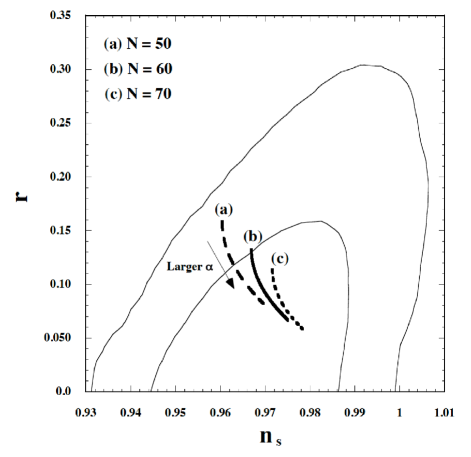
Figure 2: Observational constraints on chaotic inflation with the quadratic potential $V(\phi)=m^{2}\phi^{2}/2$ in the ($n_{\rm s},r$) plane with the three different numbers of e-foldings ($N=50,60,70$). We evaluate the theoretical values of $n_{\rm s}$ and $r$ in the range $10^{-8}\leq\alpha=m^{2}/M^{2}\leq 10^{8}$. The thin solid curves correspond to the 1$\sigma$ (inside) and 2$\sigma$ (outside) observational contours constrained by the joint data analysis of WMAP7, BAO, and HST. For larger values of $\alpha=m^{2}/M^{2}$ the tensor-to-scalar ratio $r$ gets smaller, whereas the scalar spectral index increases.

In the limit that $\alpha\to 0$ one has $x=\sqrt{2n(4N+n)}/2$ from Eqs. (20) and (21), in which case $n_{\rm s}$ and $r$ are

$$n_{\rm s} = 1-\frac{2(n+2)}{4N+n}\,,$$ (44)

$$r = \frac{16n}{4N+n}\,.$$ (45)

These values correspond to those for standard chaotic inflation. If $N=60$, then $n_{\rm s}=0.967$, $r=0.132$ for $n=2$ and $n_{\rm s}=0.951$, $r=0.262$ for $n=4$. In another limit $\alpha\to\infty$ one has $x^{n+2}=[2N(n+2)+n]n^{2}/(2\alpha)$ and

$$n_{\rm s} = 1-\frac{4(n+1)}{2(n+2)N+n}\,,$$ (46)

$$r = \frac{16n}{2(n+2)N+n}\,.$$ (47)

If $N=60$, then $n_{\rm s}=0.975$, $r=0.066$ for $n=2$ and $n_{\rm s}=0.972$, $r=0.088$ for $n=4$.

In the intermediate values of $\alpha$ between $(0,\infty)$ we need to solve Eq. (20) for $x$ by using Eq. (21). When $n=2$ the field value $x$ can be expressed as Eq. (23), in which case $n_{\rm s}$ and $r$ are known from Eqs. (42) and (43) for given values of $\alpha=m^{2}/M^{2}$ and $N$. In Fig. 2 we plot the theoretical values of $n_{\rm s}$ and $r$ for $n=2$ as a function of $\alpha$ (between $10^{-8}\leq\alpha\leq 10^{8}$) with three different values of $N\leavevmode\nobreak\ (=50,60,70)$, together with the $1\sigma$ and $2\sigma$ observational contours constrained by the joint data analysis of WMAP7 WMAP7 , BAO BAO , and HST HST . For $\alpha=10^{-8}$ these observables are close to the values estimated by Eqs. (44) and (45), whereas for $\alpha=10^{8}$ they are close to those given by Eqs. (46) and (47). For larger $\alpha$, $r$ gets smaller whereas $n_{\rm s}$ increases, so that the quadratic potential shows better compatibility with observations in the presence of the field derivative coupling to gravity.

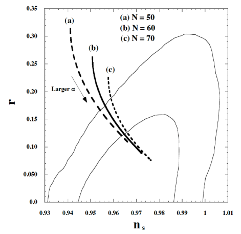
Figure 3: Observational constraints on chaotic inflation with the quartic potential $V(\phi)=\lambda\phi^{4}/4$ in the range $10^{-8}\leq\alpha=\lambda(M_{\rm pl}/M)^{2}\leq 10^{8}$ with the three different values of $N$. The $1\sigma$ and $2\sigma$ observational contours are the same as those in Fig. 2. While the standard case ($\alpha=0$) is outside the $2\sigma$ bound, the field derivative coupling to gravity can make the quartic potential compatible with observations.

In Fig. 3 the theoretical values of $n_{\rm s}$ and $r$ are plotted for $n=4$ as a function of $\alpha=\lambda(M_{\rm pl}/M)^{2}$ between $(10^{-8},10^{8})$ with $N=50,60,70$. In the limit that $\alpha\to 0$ the quartic potential is outside the $2\sigma$ observational contour for $N$ smaller than 70. In the presence of the field derivative coupling to gravity the model can be compatible with the current observations due to the suppressed tensor-to-scalar ratio and the larger spectral index. For $N=60$ the parameter $\alpha$ is constrained to be

$$\alpha>3\times 10^{-5}\leavevmode\nobreak\ \leavevmode\nobreak\ (95\,\%\leavevmode\nobreak\ {\rm CL})\,,$$ (48)

and $\alpha>4\times 10^{-4}$ (68 % CL). For $N=50$ the constraints are $\alpha>2\times 10^{-4}$ (95 % CL) and $\alpha>1\times 10^{-2}$ (68 % CL).

Using the scalar power spectrum (31), the CMB normalization by WMAP WMAP7 corresponds to

$$\frac{\alpha}{12\pi^{2}n^{4}}\left(\frac{M}{M_{\rm pl}}\right)^{2}x_{60}^{n+2}\left(n+\alpha x_{60}^{n}\right)\simeq 2.4\times 10^{-9}\,,$$ (49)

where $x_{60}$ is the value of $x$ at $N=60$. In the regime $\alpha\gg 1$ one has $x^{n+2}=[2N(n+2)+n]n^{2}/(2\alpha)$, so that Eq. (49) gives

$$\frac{m}{M_{\rm pl}} \simeq 1.5\times 10^{-10}\,\frac{M_{\rm pl}}{M}\qquad{\rm for}\leavevmode\nobreak\ \leavevmode\nobreak\ n=2\,,$$ (50)

$$\lambda \simeq 5.9\times 10^{-32}\left(\frac{M_{\rm pl}}{M}\right)^{4}\qquad{\rm for}\leavevmode\nobreak\ \leavevmode\nobreak\ n=4\,.$$ (51)

In the case of the quartic potential it is possible to realize $\lambda\simeq 0.1$ for $M\simeq 2.8\times 10^{-8}\,M_{\rm pl}$.

IV.2 Exponential potentials

Let us proceed to the exponential potential

$$V(\phi)=V_{0}\,e^{\beta\phi/M_{\rm pl}}\,,$$ (52)

where $V_{0}$ and $\beta$ are constants. In this case one has $\epsilon_{{\text{\tiny$V$}}}=\beta^{2}/2$ and $\eta_{{\text{\tiny$V$}}}=\beta^{2}$. Hence in standard slow-roll inflation we require the condition $\beta^{2}\ll 1$. Moreover this corresponds to the power-law inflation without the graceful exit earlyexp . In the presence of the field derivative coupling to gravity, however, the slow-roll parameter $\epsilon=\epsilon_{{\text{\tiny$V$}}}/{\cal A}$ can be smaller than 1 even for steep exponential potentials with $\beta^{2}\gtrsim 1$. Inflation ends when $\epsilon$ grows to the order of unity, which is followed by reheating with gravitational particle production. This situation is analogous to that in braneworld inflation where the dominance of the density squared term ($\rho^{2}$) can lead to cosmic acceleration for steep exponential potentials Copeland .

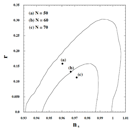
Figure 4: Observational constraints on inflation with the exponential potential $V(\phi)=V_{0}e^{\beta\phi/M_{\rm pl}}$ in the regime ${\cal A}\gg 1$ for $N=50,60,70$. The $1\sigma$ and $2\sigma$ observational contours are the same as those in Fig. 2. Even the steep exponential potentials with $\beta$ larger than 1 can be allowed from the current observational data.

We focus on the case in which the condition $V/(M^{2}M_{\rm pl}^{2})\gg 1$ is satisfied during the whole stage of inflation. Using Eq. (17) the field value $\phi_{f}$ at the end of inflation can be estimated as

$$\frac{V_{0}e^{\beta\phi_{f}/M_{\rm pl}}}{M^{2}M_{\rm pl}^{2}}\simeq\frac{\beta^{2}}{2}\,,$$ (53)

which implies that $\beta^{2}\gg 1$. From Eq. (18) it follows that

$$\frac{V_{0}e^{\beta\phi/M_{\rm pl}}}{\beta^{2}M^{2}M_{\rm pl}^{2}}\simeq N+\frac{1}{2}\,.$$ (54)

In the regime ${\cal A}\gg 1$ the scalar spectral index (32) and the tensor-to-scalar ratio (39) reduce to

$$n_{\rm s} \simeq 1-\frac{4}{2N+1}\,,$$ (55)

$$r \simeq \frac{16}{2N+1}\,,$$ (56)

which correspond to taking the limit $n\to\infty$ in Eqs. (46) and (47).

In Fig. 4 we plot the theoretical values of $n_{\rm s}$ and $r$ for $N=50,60,70$ as well as the 1$\sigma$ and 2$\sigma$ observational contours. This shows that even the steep exponential potentials with $\beta^{2}\gg 1$ are compatible with the current observational data.

Using the WMAP normalization ${\cal P}_{\rm s}\simeq 2.4\times 10^{-9}$ at $N=60$ in the regime $V/(M^{2}M_{\rm pl}^{2})\gg 1$, we obtain the constraint

$$\beta\simeq 8.8\times 10^{-6}\,\frac{M_{\rm pl}}{M}\,.$$ (57)

For $M/M_{\rm pl}\ll 10^{-5}$ one has $\beta\gg 1$.

IV.3 Natural inflation

Natural inflation Freese is described by the potential

$$V(\phi)=\Lambda^{4}\left[1+\cos\left(\frac{\phi}{f}\right)\right]\,,$$ (58)

where $\Lambda$ and $f$ are constants having the dimension of mass. In the absence of the field derivative coupling to gravity the above potential can be compatible with observational data only for $f\gtrsim 3.5M_{\rm pl}$ Savage . Then a global symmetry associated with the pseudo-Nambu-Goldstone-boson is broken above the quantum gravity scale, in which case standard quantum field theory may not be applicable. If the potential (58) originates from the string axion, the regime $f\gtrsim M_{\rm pl}$ is not generally realized Banks . This problem can be circumvented by taking into account the field derivative coupling to gravity Germani2 .

In the following we focus on the case in which the condition ${\cal A}\gg 1$ is satisfied during the whole stage of inflation ($0<\phi<\pi f$). From Eq. (17) the end of inflation is characterized by

$$\cos\chi_{f}\simeq-1+\frac{\sqrt{16\gamma+1}-1}{4\gamma}\,,$$ (59)

where $\chi_{f}=\phi_{f}/f$ and

$$\gamma=\frac{f^{2}\Lambda^{4}}{M^{2}M_{\rm pl}^{4}}\,.$$ (60)

The number of e-foldings is given by

$$N\simeq\gamma\left[{\cal F}(\chi_{f})-{\cal F}(\chi)\right]\,,$$ (61)

where $\chi=\phi/f$ and

$${\cal F}(\chi)=2\ln\left(\frac{1}{\sin\chi}-\frac{1}{\tan\chi}\right)+2\ln\,(\sin\chi)+\cos\chi\,.$$ (62)

The scalar spectral index and the tensor-to-scalar ratio are

$$n_{\rm s} = 1-\frac{2}{\gamma}\frac{2-\cos\chi}{(1+\cos\chi)^{2}}\,,$$ (63)

$$r = \frac{8}{\gamma}\frac{1-\cos\chi}{(1+\cos\chi)^{2}}\,.$$ (64)

For given $\gamma$ the field value $\chi_{f}$ is known from Eq. (59). Since $\chi$ is determined by Eq. (61) for given values of $\gamma$ and $N$, we can numerically evaluate $n_{\rm s}$ and $r$ as functions of $\gamma$ for several different numbers of e-foldings. In Fig. 5 we plot $n_{\rm s}$ and $r$ in the range $7\leq\gamma\leq 10^{6}$, together with the 1$\sigma$ and $2\sigma$ observational contours. For increasing $\gamma$, both $n_{\rm s}$ and $r$ get larger.

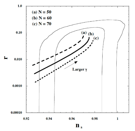
Figure 5: Observational constraints on natural inflation with the potential $V(\phi)=\Lambda^{4}\left[1+\cos\left(\phi/f\right)\right]$ in the range $7\leq\gamma=f^{2}\Lambda^{4}/(M^{2}M_{\rm pl}^{4})\leq 10^{6}$ with ${\cal A}\gg 1$ for three different values of $N$. The $1\sigma$ and $2\sigma$ observational contours are the same as those in Fig. 2. For larger $\gamma$, both $n_{\rm s}$ and $r$ increase toward the values $n_{\rm s}=1-6/(4N+1)$ and $r=16/(4N+1)$.

In the limit that $\gamma\gg 1$ it is possible to estimate $n_{\rm s}$ and $r$ analytically. From Eq. (59) one has $\cos\chi_{f}\simeq-1+1/\sqrt{\gamma}$ and hence $\chi_{f}$ is close to $\pi$, as $(\pi-\chi_{f})^{4}\simeq 4/\gamma$. Using Eq. (61), it follows that $N\simeq(\gamma/16)(\pi-\chi)^{4}-1/4$. Then Eqs. (63) and (64) reduce to

$$n_{\rm s} \simeq 1-\frac{6}{4N+1}\,,$$ (65)

$$r \simeq \frac{16}{4N+1}\,.$$ (66)

These values correspond to $n=2$ in Eqs. (46) and (47). This comes from the fact that in the regime $\gamma\gg 1$ inflation occurs around the potential minimum at $\phi=\pi f$. As in the case of the quadratic potential $V(\phi)=m^{2}\phi^{2}/2$ with $\alpha=m^{2}/M^{2}\gg 1$, natural inflation with $\gamma\gg 1$ is compatible with the current observations.

For $N=60$ the parameter $\gamma$ is constrained to be

$$\gamma>7.5\leavevmode\nobreak\ \leavevmode\nobreak\ (95\,\%\leavevmode\nobreak\ {\rm CL})\,,$$ (67)

and $\gamma>9.8$ (68 % CL). For $N=50$ the constraints are $\gamma>7.8$ (95 % CL) and $\gamma>10.6$ (68 % CL). In the regime $\gamma\gg 1$ the WMAP normalization at $N=60$ gives

$$f\simeq 8\times 10^{4}\,\gamma^{1/4}\,M\,.$$ (68)

If $M\lesssim 10^{-5}\gamma^{-1/4}M_{\rm pl}$, then one has $f\lesssim M_{\rm pl}$.

IV.4 Hybrid inflation

Finally we study hybrid inflation with the potential

$$V(\phi)=V_{0}+\frac{1}{2}m^{2}\phi^{2}\,,$$ (69)

where $V_{0}$ and $m$ are constants. Inflation ends at a bifurcation point given by $\phi=\phi_{c}$ due to the appearance of a tachyonic instability driven by another field $\chi$. As in the case of the original hybrid inflation hybrid we focus on the regime $V_{0}\gg m^{2}\phi^{2}/2$. Note that in another regime $V_{0}\ll m^{2}\phi^{2}/2$ the situation is similar to that in chaotic inflation discussed in Sec. IV.1.

Using Eq. (18) the field value can be estimated as

$$\phi\simeq\phi_{c}\exp\left(\frac{\nu}{1+\mu}N\right)\,,$$ (70)

where $\mu$ and $\nu$ are positive constants defined by

$$\mu=\frac{V_{0}}{M^{2}M_{\rm pl}^{2}}\,,\qquad\nu=\frac{m^{2}M_{\rm pl}^{2}}{V_{0}}\,.$$ (71)

From Eqs. (32) and (39) we obtain

$$n_{\rm s} \simeq 1+\frac{2\nu}{1+\mu}\,,$$ (72)

$$r \simeq \frac{8\nu^{2}}{1+\mu}\left(\frac{\phi_{c}}{M_{\rm pl}}\right)^{2}\,e^{(n_{\rm s}-1)N}\,,$$ (73)

which mean that the scalar power spectrum is blued-tilted ($n_{\rm s}>1$). Compared to the standard hybrid inflation, the presence of the field derivative coupling to gravity ($\mu>0$) leads to $n_{\rm s}$ close to 1 as well as the suppressed tensor-to-scalar ratio. In the limit that $\mu\gg 1$ one has $n_{\rm s}\to 1$ and $r\to 0$, i.e. the Harrison-Zel’dovich (HZ) spectrum. The HZ spectrum is under the observational pressure WMAP7 , but this property is subject to change depending on the assumptions about the reionization scenario reion . The future high-precision observations will provide a more concrete answer about this issue.

In the regime $\mu\gg 1$ and $\nu\ll 1$ one has $\phi\simeq\phi_{c}$ for $N\sim 60$. From the WMAP normalization it follows that

$$\frac{\mu}{\nu}\frac{M}{\phi_{c}}\simeq 5.3\times 10^{-4}\,.$$ (74)

If $\mu=10^{2}$, $\nu=10^{-2}$, $\phi_{c}=0.2M_{\rm pl}$, for example, $M\simeq 10^{-8}$ GeV. In this case Eqs. (72) and (73) give $n_{\rm s}\simeq 1.0002$ and $r\simeq 3\times 10^{-7}$, which is close to the HZ spectrum.

V Conclusions

In this paper we have studied observational constraints on a number of representative inflationary models with a field derivative coupling to the Einstein tensor, i.e. $G^{\mu\nu}\partial_{\mu}\phi\partial_{\nu}\phi/(2M^{2})$. Such a non-minimal derivative coupling has an asymptotic local shift symmetry for a slow-rolling scalar field satisfying the condition $\varepsilon=(\partial\phi)^{2}/(M^{2}M_{\rm pl}^{2})\ll 1$. Since the strong coupling scale of the theory is around the Planck scale for $\varepsilon\ll 1$, quantum corrections to the inflaton potential can be suppressed during inflation.

The non-minimal derivative coupling to gravity leads to a gravitationally enhanced friction for the scalar field. This property allows us to accommodate steep potentials with theoretically natural model parameters for realizing inflation. Not only the quartic potential $V(\phi)=\lambda\phi^{4}/4$ with $\lambda\sim 0.1$ but the potential $V(\phi)=\Lambda^{4}[1+\cos(\phi/f)]$ with $f\ll M_{\rm pl}$ gives rise to cosmic acceleration consistent with the amplitude of the CMB temperature anisotropies. Moreover the exponential potential $V(\phi)=V_{0}e^{\beta\phi/M_{\rm pl}}$, which often appears after the compactification of extra dimensions in higher-dimensional theories, can lead to inflation even for $\beta^{2}\gg 1$ in the presence of the field derivative coupling to gravity.

For the potential $V(\phi)=(\lambda/n)\phi^{n}$ of chaotic inflation the tensor-to-scalar ratio $r$ decreases for larger $\alpha=\lambda M_{\rm pl}^{n-2}/M^{2}$, whereas the scalar spectral index $n_{\rm s}$ increases. In the limit that $\alpha\to\infty$, $n_{\rm s}$ and $r$ approach the values given in Eqs. (46) and (47). As we see in Figs. 2 and 3, for both $n=2$ and $n=4$, the asymptotic values of $n_{\rm s}$ and $r$ are within the $1\sigma$ observational bound derived by the joint data analysis of WMAP7, BAO, and HST. For the quartic potential with $N=60$ we found that the parameter $\alpha=\lambda(M_{\rm pl}/M)^{2}$ is constrained to be $\alpha>3\times 10^{-5}$ at the 95 % confidence level.

For the exponential potential $V(\phi)=V_{0}e^{\beta\phi/M_{\rm pl}}$ the asymptotic values of $n_{\rm s}$ and $r$ in the regime $V/(M^{2}M_{\rm pl}^{2})\gg 1$ are given by Eqs. (55) and (56), with $\beta$ constrained as Eq. (57) from the WMAP normalization. Figure 4 shows that steep exponential potentials with $\beta^{2}\gg 1$ can be compatible with the current observational data.

In natural inflation with the potential $V(\phi)=\Lambda^{4}[1+\cos(\phi/f)]$ the observables can be parametrized by the parameter $\gamma=f^{2}\Lambda^{4}/(M^{2}M_{\rm pl}^{4})$ in the regime $V/(M^{2}M_{\rm pl}^{2})\gg 1$. For larger $\gamma$, both $n_{\rm s}$ and $r$ tend to increase toward the values given in Eqs. (65) and (66). These asymptotic values correspond to those derived in Eqs. (46) and (47) for $n=2$ with $\alpha\gg 1$. This property comes from the fact that for $\gamma\gg 1$ inflation occurs around the potential minimum at $\phi=\pi f$. The observational bound on the parameter $\gamma$ is found to be $\gamma>7.5$ for $N=60$ (95 % CL). From the WMAP normalization the symmetry breaking scale $f$ is constrained to be $f\simeq 8\times 10^{4}\,\gamma^{1/4}M$, which can be smaller than $M_{\rm pl}$ for $M\lesssim 10^{-5}\gamma^{-1/4}M_{\rm pl}$.

In hybrid inflation with the potential $V(\phi)=V_{0}+m^{2}\phi^{2}/2$ (where $V_{0}\gg m^{2}\phi^{2}/2$) the field derivative coupling to gravity leads to the blue-tilted scalar power spectrum close to $n_{\rm s}=1$. Compared to standard hybrid inflation, the power spectrum approaches the HZ one, i.e. $n_{\rm s}=1$ and $r=0$. The HZ spectrum is in tension with observations, but we have to caution that this property is affected by the assumption of the reionization scenario.

If future observations such as PLANCK PLANCK can constrain the tensor-to-scalar ratio at the level of $r\lesssim{\cal O}(0.01)$, this will allow us to place tighter bounds on the inflationary models with the field derivative coupling to gravity. We hope that we can discriminate between a host of inflationary models within the next few years.

References

- (1) A. A. Starobinsky, Phys. Lett. B 91, 99 (1980); D. Kazanas, Astrophys. J. 241, L59 (1980); K. Sato, Mon. Not. R. Astron. Soc. 195, 467 (1981); A. H. Guth, Phys. Rev. D 23, 347 (1981).
- (2) A. D. Linde, Phys. Lett. B 108, 389 (1982); A. Albrecht and P. J. Steinhardt, Phys. Rev. Lett. 48, 1220 (1982).
- (3) A. D. Linde, Phys. Lett. B 129, 177 (1983).
- (4) V. F. Mukhanov and G. V. Chibisov, JETP Lett. 33, 532 (1981); A. H. Guth and S. Y. Pi, Phys. Rev. Lett. 49, 1110 (1982); S. W. Hawking, Phys. Lett. B 115, 295 (1982); A. A. Starobinsky, Phys. Lett. B 117, 175 (1982); J. M. Bardeen, P. J. Steinhardt and M. S. Turner, Phys. Rev. D 28, 679 (1983).
- (5) G. F. Smoot et al., Astrophys. J. 396, L1 (1992).
- (6) E. Komatsu et al. [WMAP Collaboration], Astrophys. J. Suppl. 192, 18 (2011).
- (7) A. R. Liddle and D. H. Lyth, “Cosmological inflation and large scale structure,” Cambridge, UK: Univ. Pr. (2000).
- (8) A. D. Linde, “Particle physics and inflationary cosmology,” Chur, Switzerland: Harwood (1990) [hep-th/0503203]; D. H. Lyth and A. Riotto, Phys. Rept. 314, 1 (1999).
- (9) C. Amsler et al. [Particle Data Group Collaboration], Phys. Lett. B 667, 1 (2008).
- (10) F. L. Bezrukov and M. Shaposhnikov, Phys. Lett. B 659, 703 (2008).
- (11) T. Futamase and K. -i. Maeda, Phys. Rev. D 39, 399 (1989); R. Fakir and W. G. Unruh, Phys. Rev. D 41, 1783 (1990).
- (12) D. S. Salopek, J. R. Bond and J. M. Bardeen, Phys. Rev. D 40, 1753 (1989); N. Makino and M. Sasaki, Prog. Theor. Phys. 86, 103 (1991); D. I. Kaiser, Phys. Rev. D 52, 4295 (1995); E. Komatsu and T. Futamase, Phys. Rev. D 59, 064029 (1999); S. Tsujikawa and B. Gumjudpai, Phys. Rev. D 69, 123523 (2004).
- (13) C. P. Burgess, H. M. Lee and M. Trott, JHEP 0909, 103 (2009); J. L. F. Barbon and J. R. Espinosa, Phys. Rev. D 79, 081302 (2009); M. P. Hertzberg, JHEP 1011, 023 (2010); G. F. Giudice and H. M. Lee, Phys. Lett. B 694, 294 (2011); R. N. Lerner and J. McDonald, arXiv:1112.0954 [hep-ph].
- (14) C. Germani and A. Kehagias, Phys. Rev. Lett. 105, 011302 (2010).
- (15) L. Amendola, Phys. Lett. B 301, 175 (1993).
- (16) C. Germani and A. Kehagias, JCAP 1005, 019 (2010).
- (17) C. Germani and A. Kehagias, Phys. Rev. Lett. 106, 161302 (2011).
- (18) C. Germani and Y. Watanabe, JCAP 1107, 031 (2011).
- (19) C. Germani, L. Martucci and P. Moyassari, arXiv:1108.1406 [hep-th].
- (20) A. Nicolis, R. Rattazzi and E. Trincherini, Phys. Rev. D 79, 064036 (2009).
- (21) C. Deffayet, G. Esposito-Farese and A. Vikman, Phys. Rev. D 79, 084003 (2009); C. Deffayet, S. Deser and G. Esposito-Farese, Phys. Rev. D 80, 064015 (2009).
- (22) K. Kamada, T. Kobayashi, M. Yamaguchi and J. ’i. Yokoyama, Phys. Rev. D 83, 083515 (2011).
- (23) T. Kobayashi, M. Yamaguchi and J. Yokoyama, Phys. Rev. Lett. 105, 231302 (2010); C. Burrage, C. de Rham, D. Seery and A. J. Tolley, JCAP 1101, 014 (2011); S. Mizuno and K. Koyama, Phys. Rev. D82, 103518 (2010); A. De Felice and S. Tsujikawa, Phys. Rev. Lett. 105, 111301 (2010); Phys. Rev. D 84, 124029 (2011); P. Creminelli et al., JCAP 1102, 006 (2011). A. Naruko and M. Sasaki, Class. Quant. Grav. 28, 072001 (2011); A. De Felice and S. Tsujikawa, JCAP 1104, 029 (2011); T. Kobayashi, M. Yamaguchi and J. Yokoyama, Phys. Rev. D83, 103524 (2011); A. De Felice, S. Tsujikawa, J. Elliston and R. Tavakol, JCAP 1108, 021 (2011).
- (24) K. Freese, J. A. Frieman and A. V. Olinto, Phys. Rev. Lett. 65, 3233 (1990); F. C. Adams et al., Phys. Rev. D 47, 426 (1993).
- (25) C. Savage, K. Freese and W. H. Kinney, Phys. Rev. D 74, 123511 (2006).
- (26) R. Kallosh, A. D. Linde, D. A. Linde and L. Susskind, Phys. Rev. D 52, 912 (1995); N. Arkani-Hamed, H. -C. Cheng, P. Creminelli and L. Randall, Phys. Rev. Lett. 90, 221302 (2003).
- (27) F. Lucchin and S. Matarrese, Phys. Rev. D 32, 1316 (1985); J. J. Halliwell, Phys. Lett. B 185, 341 (1987); J. Yokoyama and K. i. Maeda, Phys. Lett. B 207, 31 (1988); A. B. Burd and J. D. Barrow, Nucl. Phys. B 308, 929 (1988).
- (28) M. B. Green, J. H. Schwarz and E. Witten, Superstring Theory, Cambridge University Press (1987); K. A. Olive, Phys. Rep. 190, 308 (1990); E. Bergshoeff, M. de Roo, M. B. Green, G. Papadopoulos and P. K. Townsend, Nucl. Phys. B 470, 113 (1996); P. Kanti and K. A. Olive, Phys. Rev. D 60, 043502 (1999).
- (29) T. Kobayashi, M. Yamaguchi and J. Yokoyama, Prog. Theor. Phys. 126, 511 (2011).
- (30) X. Gao and D. A. Steer, JCAP 1112, 019 (2011).
- (31) A. De Felice and S. Tsujikawa, Phys. Rev. D 84, 083504 (2011).
- (32) W. Percival et al., Mon. Not. R. Astron. Soc. 401, 2148 (2010).
- (33) A. G. Riess et al., Astrophys. J. 699, 539 (2009).
- (34) L. A. Popa, JCAP 1110, 025 (2011).
- (35) A. D. Linde, Phys. Rev. D 49, 748 (1994).
- (36) G. W. Horndeski, Int. J. Theor. Phys. 10, 363-384 (1974).
- (37) C. Deffayet, X. Gao, D. A. Steer and G. Zahariade, Phys. Rev. D 84, 064039 (2011).
- (38) C. Charmousis, E. J. Copeland, A. Padilla and P. M. Saffin, Phys. Rev. Lett. 108, 051101 (2012).
- (39) A. De Felice and S. Tsujikawa, JCAP 1202, 007 (2012).
- (40) M. A. Luty, M. Porrati and R. Rattazzi, JHEP 0309, 029 (2003); K. Hinterbichler, M. Trodden and D. Wesley, Phys. Rev. D 82, 124018 (2010).
- (41) J. M. Bardeen, Phys. Rev. D 22, 1882 (1980); H. Kodama and M. Sasaki, Prog. Theor. Phys. Suppl. 78, 1 (1984); V. F. Mukhanov, H. A. Feldman and R. H. Brandenberger, Phys. Rept. 215, 203 (1992); B. A. Bassett, S. Tsujikawa and D. Wands, Rev. Mod. Phys. 78, 537 (2006).
- (42) E. J. Copeland, A. R. Liddle and J. E. Lidsey, Phys. Rev. D 64, 023509 (2001)
- (43) T. Banks, M. Dine, P. J. Fox and E. Gorbatov, JCAP 0306, 001 (2003); N. Barnaby and M. Peloso, Phys. Rev. Lett. 106, 181301 (2011).
- (44) J. E. Kim, H. P. Nilles and M. Peloso, JCAP 0501, 005 (2005); S. Dimopoulos, S. Kachru, J. McGreevy and J. G. Wacker, JCAP 0808, 003 (2008); L. McAllister, E. Silverstein and A. Westphal, Phys. Rev. D 82, 046003 (2010).
- (45) S. Pandolfi et al., Phys. Rev. D 81, 123509 (2010); Phys. Rev. D 82, 123527 (2010).
- (46) [PLANCK Collaboration], arXiv:astro-ph/0604069.